Noise-induced macroscopic bifurcations in globally-coupled chaotic units

Abstract

Large populations of globally-coupled identical maps subjected to independent additive noise are shown to undergo qualitative changes as the features of the stochastic process are varied. We show that for strong coupling, the collective dynamics can be described in terms of a few effective macroscopic degrees of freedom, whose deterministic equations of motion are systematically derived through an order parameter expansion.

Dynamical units coupled all-to-all constitute relevant models of a wide range of physical and biological systems such as Josephson junction arrays josephson , electrochemical oscillators kiss02 , interacting neurons sompolinsky91 and yeast cells in a continuous-flow, stirred tank reactor dano99 . Globally-coupled dynamical systems are also widely used as prototypical models for addressing the collective behavior of systems with many degrees of freedom mapspop . In the limit of strong coupling of identical units, full synchronization usually occurs, i.e. the collective dynamics is an exact copy of the individual one. However, in the generic case where some diversity and/or noise is present at the microscopic level, macroscopic measurements do not directly reflect individual dynamical features. This simple observation is of large experimental importance. In the yeast cell experiment, for instance, single-cell measurements are not available so far. The idea is thus to extract information about metabolic processes at the individual level from the observed collective oscillations in cell suspensions dano99 .

In this Letter, we consider the influence of microscopic additive noise on the fully-synchronous regime of globally-coupled systems. This allows us to isolate the effect of noise from the possibly already complex collective dynamics that systems of globally-coupled identical and noiseless units may themselves exhibit mapspop . Restricting, for simplicity, our discussion to identical scalar maps, we show that noise plays a non-trivial role, “unfolding” the noiseless collective dynamics while progressively suppressing the direct connection between average and local evolution. We build a systematic expansion that accounts quantitatively for the collective dynamics observed, revealing that its essential features can be described in terms of few effective degrees of freedom and that its hierarchical structure is captured in progressively greater detail as the truncation order is increased.

Our system of noisy and globally coupled identical one-dimensional maps is defined as follows:

$$x_{j}\mapsto(1-K)\,f(x_{j})+K\,\langle\,{f(x)}\,\rangle+\xi_{j}(t)\quad j=1,\dots N,$$ (1)

where $x_{j}\in\mathbb{R}$ denotes the state of the j-th population element, $f:\mathbb{R}\rightarrow\mathbb{R}$ is a smooth function defining the dynamics of the uncoupled element, and $\langle\,{f(x)}\,\rangle:=\frac{1}{N}\sum_{j=1}^{N}\,f(x_{j})$ is the average over the population. Every map is subjected to a white, but not necessarily Gaussian, noise of zero average and variance $\sigma^{2}$.

Without noise and for strong enough coupling, the trajectories of all the population elements asymptotically coincide (full synchronization). The mean field $X=\langle x\rangle$ then evolves on a one-dimensional manifold of the high-dimensional phase space of the full system.

Although noise smears any individual trajectory, for large population sizes these fluctuations average out and the mean field $X$ evolves deterministically up to finite-size effects. Somewhat counter-intuitively, the macroscopic dynamics is qualitatively different from that of the uncoupled map and remains apparently low-dimensional for any noise intensity. For chaotic logistic maps, increasing noise drives the mean field $X$ through a cascade of period-doubling bifurcations which takes place at smaller and smaller $\sigma$ values as the coupling strength $K$ is lowered (Fig. 1 (d-f)). The difference between single element noisy evolution and regular average behaviour can be easly seen comparing the sharply peaked probability distribution functions (pdf) of $X$ with the broad, smooth pdfs of individual elements (Fig. 1 (a-c)).

The effect of noise is not always the “simplification” of the collective dynamics; rather, noise unravels the underlying complexity of the phase space. This is particularly striking in the case of excitable units, such as:

$$f(x)=(\alpha\,x+\gamma\,x^{3})\>e^{-\beta\,x^{2}}.$$ (2)

(For other examples of excitable maps, see excmaps .) While the origin is the unique global attractor, map (2) possesses an unstable fixed point, excitation across which triggers a chaotic transient. Increasing the noise intensity over a threshold $\sigma^{*}$, the mean field displays intermittent bursts, due to the crisis of a chaotic attractor which disappears, for stronger noise, via a period-doubling cascade (Fig. 2). The onset of collective oscillations is nothing but an explicit mechanism for “noise-induced” and “coherence” resonance cohres : the single-element power spectrum displays an enhanced peak in the periodic regimes occurring at intermediate $\sigma$ valuestbp .

Figure 1: System of $N=2^{20}$ globally coupled logistic maps in the chaotic regime ($f(x)=1-a\,x^{2}$, $a=1.57$) subjected to uniformly-distributed noise of variance $\sigma^{2}$. (a-c): $K=0.7$: pdfs for the mean field (solid line) and one single element (dash-dotted line; dotted line at even times, dashed line at odd times) for different noise intensities: (a) $\sigma^{2}=0.0025$, (b) $\sigma^{2}=0.0324$, and (c) $\sigma^{2}=0.09$. (d): Bifurcation diagram for $X$ as a function of $\sigma^{2}$ for $K=1$. (e): First period-doubling bifurcations for the mean field ($\circ$) and for the second-order reduced system (solid line, see text) in the $(\sigma,K)$ plane. (f): Same as (d) but for the reduced system Eq.(Noise-induced macroscopic bifurcations in globally-coupled chaotic units) with $K=0.7$ (the diagram of the full system almost coincides). The dotted lines in (d) and (f) indicate the location of the bifurcations reported in (e).

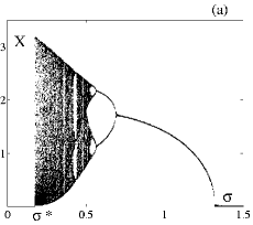
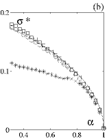
Figure 2: Population of $N=2^{22}$ excitable maps (Eq. (2) with $\alpha=0.4$, $\beta=1$, $\gamma=8$, and $K=0.9$) subjected to Gaussian noise of variance $\sigma^{2}$. (a): Bifurcation diagram for $X$ vs $\sigma$. (b): Critical value $\sigma^{*}$ of the noise intensity over which the mean field displays large amplitude oscillations for the population ($K=1$,$\square$; $K=0.8$, $\circ$; $K=0.6$, $*$) and for the order parameter reduction (solid line).

Let us now investigate analytically the apparent low-dimensional nature of the collective motion by trying to decouple the macroscopic effect of noise from the dynamical “skeleton” provided by the microscopic map. We write the position of each population element in terms of the mean field and of its displacement from it: $x_{j}=X+\epsilon_{j}$. The uncoupled element equation can now be expanded as a power series around the mean field:

$$f(x_{j})=f(X)+\sum_{q=1}^{\infty}\>\frac{1}{q!}\>\mathcal{D}^{q}f(X)\>\epsilon_{j}^{q},$$ (3)

where $\mathcal{D}^{q}f$ indicates the $q$-th derivative of the function $f$. Substituting Eq. (3) into Eq. (1), the macroscopic first iterate is obtained by averaging:

$$X\mapsto\langle\,{f(x)}\,\rangle=f(X)+\sum_{q=1}^{\infty}\>\frac{1}{q!}\>\mathcal{D}^{q}f(X)\>\langle\,{\epsilon^{q}}\,\rangle\;.$$ (4)

The mean field is then coupled to a full set of new order parameters:

$$\Omega_{q}:=\langle\,{\epsilon^{q}}\,\rangle\hskip 56.9055ptq\in\mathbb{N}.$$ (5)

It is worth stressing that, at this point, we have taken the infinite-size limit, discarding the term $\langle\,{\xi}\,\rangle$ which scales like $1/\sqrt{N}$ and plays the role of a macroscopic noise acting on the mean-field. This accounts for the mean field fluctuations obeying the law of large numbers.
The evolution of the order parameters $\Omega_{q}$ can be computed using:

$$\epsilon_{j}\mapsto(1-K)\>\sum_{p=1}^{\infty}\>\frac{1}{p!}\>\mathcal{D}^{p}f(X)\>\left(\epsilon_{j}^{p}-\Omega_{p}\right)+\xi_{j}$$

and the fact that, in the limit $N\to\infty$, the positions and the noise are uncorrelated variables and, hence, $\langle\,{h(X,\epsilon)\>\xi^{q}}\,\rangle=\langle\,{h(X,\epsilon)}\,\rangle\>\langle\,{\xi^{q}}\,\rangle$. Eq. (5) then yields:

$$\Omega_{q}\mapsto m_{q}+ \sum_{i=1}^{q}\binom{q}{i}(1-K)^{i}m_{q-i}$$ (6)

$$\left\langle\left[\sum_{p=1}^{\infty}\frac{1}{p!}\mathcal{D}^{p}f(X)\left(\epsilon^{p}-\Omega_{p}\right)\right]^{i}\right\rangle,$$

where $m_{q}=\langle\,{\xi^{q}}\,\rangle$ is the $q$-th moment of the noise distribution. The macroscopic dynamical system defined by Eqs. (4) and (6) is still infinite-dimensional, like the full system, but it can be truncated to finite-order when assuming that $1-K$ is sufficiently small. This leads to a hierarchy of finite-dimensional reduced systems which capture, as we show below, the properties of the collective dynamics in increasing detail.

A first approximation of Eq. (6) consists in keeping only terms of zeroth order in $(1-K)$, so that any $\Omega_{q}=m_{q}$. The scalar equation for the mean field:

$$X\mapsto f(X)+\sum_{q=1}^{\infty}\>\frac{1}{q!}\>\mathcal{D}^{q}f(X)\>m_{q}$$ (7)

describes exactly the bifurcation diagram for $K=1$ Fig. 1 (d). Here, the macroscopic effect of noise is a one-dimensional unfolding of the uncoupled element dynamics, whose nonlinearities become progressively more relevant as the noise intensity increases. In particular, if the map is polynomial, only a finite number of moments influence the mean-field dynamics. This suggests a criterium for dividing the noise distributions into classes according to the collective behaviour they generate.

For logistic maps, Eq. (7) takes the simple form:

$$X\mapsto 1-a\>\sigma^{2}-a\>X^{2}.$$ (8)

This map is easily rescaled to a logistic map in which $\sigma^{2}$ plays the role of the usual nonlinearity parameter. Although Eq. (8) provides a good approximation to the regimes of very strong coupling, it is independent of $K$. Hence, it cannot account for the changes with $K$ of the period-doubling bifurcation lines (Fig. 1(e)). Truncating Eqs. (4) and (6) to the second order in $(1-K)$ (the first order term vanishes for zero-average noise) the coupling strength appears as a parameter for the macroscopic equations of motion. In this case, the higher-order moments obey a recurrence relation leading, when $f$ is polynomial, to a two-dimensional map. For our example of logistic maps, this reads:

$$X\mapsto 1-a\,X^{2}-a\>\Omega_{2}$$

$$\Omega_{2}\mapsto \sigma^{2}+(1-K)^{2}a^{2}$$

$$\times\left[m_{4}-6\sigma^{4}+(4X^{2}-\Omega_{2}+6\sigma^{2})\Omega_{2}\right].$$

Figure 1(e) shows that even for intermediate coupling strengths this equation accounts quantitatively for the main features of the mean field dynamics.
Looking at the bifurcation cascade of Fig. 1 (f), one could think that Eqs. (Noise-induced macroscopic bifurcations in globally-coupled chaotic units) might be further reduced to a scalar map. This is not possible, however, as the mean field first return map is folded (Fig. 3) and hence the macroscopic system must have more than one variable. Remarkably, our approximation at order $(1-K)^{2}$ (Eq. (Noise-induced macroscopic bifurcations in globally-coupled chaotic units) for logistic maps) reproduces this folded structure. For both the full system and the second-order approximation Eq. (Noise-induced macroscopic bifurcations in globally-coupled chaotic units), the distance $d_{X}$ between the first return map of $X$ and the parabola identified by the zeroth order truncation scales, as expected, like $(1-K)^{2}$ or $\sigma^{2}$ (Fig. 3(c,d)) and vanishes on $K=1$, where the zeroth-order truncation Eq. (8) is exact. The “thickness” of the transverse folded structure shown in Fig. 3(a) scales similarly tbp , indicating that, apart from finite-size effects that may prevent us from observing it, the dimension of the macroscopic attractor becomes larger than that of the uncoupled element as soon as $K<1$ and $\sigma>0$.
Going one step further, it is easily seen that there are still features of the mean field dynamics that cannot be captured by Eq. (Noise-induced macroscopic bifurcations in globally-coupled chaotic units). The macroscopic variables $\Omega_{q}$ for the population satisfy only approximately the relations used for reducing the dimensionality of the truncated system. For instance, $\Omega_{4}$ displays a complex dependence on $\Omega_{2}$ (Fig. 3(b)), while it is constant at zeroth order, and linear at second-order. In turn, this complex structure is retrieved if Eqs. (4) and (6) are truncated to fourth order in $(1-K)$. In the $(\Omega_{2},\Omega_{4})$ plane, the distances $d_{\Omega}$ separating the second-order truncation from the full system or the fourth-order truncation are comparable and they scale like the expected $(1-K)^{4}$ and $\sigma^{4}$ (Figs. 3(c,d)).

Figure 3: Population of Fig. 1 (a): First return map of $X$ for the full system (dark dots), its zeroth-order approximation (solid line), and its second-order approximation (light dots) ($K=0.4$ and $\sigma^{2}=0.001$). (b): $\Omega_{4}$ versus $\Omega_{2}$ for the same parameters (dark dots: full system, zeroth-order: triangle, second-order: solid line, fourth-order: light dots). (c) and (d) distances $d_{x}$ and $d_{\Omega}$ defined in text (circles for the full system, dashed lines for the second-order approximation, solid line for fourth-order system). ((c): $\sigma^{2}=0.03$; (d): $K=0.6$).

Extrapolating from the above results, we conclude that the presence of noise unfolds the fully-synchronized regime into an infinitely complex but hierarchically organized structure whose main features are captured by the lowest orders of our approximation scheme. Nevertheless, in the parameter region considered here, we expect the collective chaos to remain embedded in a finite dimensional space. This is perhaps best seen when calculating the Lyapunov exponents of the finite-dimensional maps approximating the full system. The maps possess only one positive exponent in the chaotic region, whereas increasing the order of the approximation adds “new”, more negative exponents to those existing at previous order. These exponent values agree well with those numerically computed by simulating the Perron-Frobenius dynamics of the population pdf tbp , so that we are confident that they do represent the collective dynamics of the full system.

In general, when the local map $f$ is not polynomial, the order parameter expansion of Eq. (2) contains an infinite number of terms even for $K=1$, and it is then necessary to introduce the further closure assumption $\sigma\ll 1$ to obtain closed form approximations. We can illustrate this for the excitable map example mentioned above. At second order in both $(1-K)$ and $\sigma$, the approximation accounts well for the establishment of collective oscillations. The linear stability analysis of the origin for the reduced system provides an analytical condition for the onset of the intermittent behavior, which is in good agreement with the simulations of the population (Fig. 2 (b)).

To summarize, the collective dynamics of infinitely-large populations of globally-coupled identical maps subjected to independent additive noise is deterministic and undergoes qualitative changes as the features of the stochastic process are varied. For strong coupling, the collective dynamics can be described in terms of a few effective macroscopic degrees of freedom, whose equations of motion have been systematically derived through an order parameter expansion valid for any smooth map and noise distribution. Such a reduced system allows us to understand how the nonlinearities of the map interact with the specific features of the microscopic noise. At the experimental level, our work indicates that the observation of unusual pdfs of local variables such a those shown in Fig. 1 may be traced back to the presence of an underlying chaotic local dynamics.

Our approach reveals that in a large region of parameter space the collective motion, in spite of being endowed with a single positive Lyapunov exponent, takes place on a hierarchically-organized complex attractor. We believe that this complexity is but another facet of the “anomalous scaling” properties of the cloud of points representing the population in the local phase space which were uncovered recently by Teramae and Kuramoto teramae01 , both phenomena being rooted in the structure of the global phase space around the fully-synchronized solution.

The method proposed here, together with Ref. our , allows to compare the macroscopic bifurcations induced by different sources of microscopic disorder, such as noise and parameter mismatch (quenched noise). In this last case, an order parameter expansion with other closure assumptions provides a different low-dimensional unfolding of the local dynamics, accounting for the observed diversity of the bifurcation scenarios tbp .

Future work should consider how all these aspects evolve as one lowers the coupling strength towards the weak-coupling regimes considered by Shibata et al. shibata99 where collective chaos is high-dimensional. Our work can be extended to the case of continuous-time systems, where we expect a similar effect of microscopic noise continuous . Finally, it would be most interesting to make the connection with lattices or networks of locally-coupled maps, and the so-called non-trivial collective behavior they exhibit. There, as suggested in lemaitre , the equivalent of the noise considered here lies in the finite-amplitude fluctuations introduced by the neighbors and the finite correlation length in the system.

S.D.M. acknowledges support from the ESF Programme REACTOR. The authors are grateful to the referees for their comments.

References

- (1) P. Hadley, M. R. Beasley, and K. Wiesenfeld, Phys. Rev. B 38, 8712 (1988); S. Nichols and K. Wiesenfeld, Phys. Rev. E 49, 1865 (1994).
- (2) I. Z. Kiss, Y. Zhai, and J. L. Hudson, Science 296, 1677 (2002).
- (3) S. Danø, P. G. Sørensen, and F. Hynne, Nature 402, 320 (1999).
- (4) H. Sompolinsky, D. Golomb, and D. Kleinfeld, Phys. Rev. A 43, 6990 (1991).
- (5) A. T. Winfree, The Geometry of Biological Time, (Springer, New York, 1980).
- (6) K. Kaneko, Phys. Rev. Lett. 63, 219 (1989); Physica D 41, 137 (1990); A. S. Pikovsky and J. Kurths, ibid. 72, 1644 (1994); T. Shimada and S. Tsukada, Physica D 168-169, 126 (2002); O. Popovytch, Y. Maistrenko, and E. Mosekilde, Phys. Lett. A 302, 171 (2002).
- (7) R. Toral, C. R. Mirasso, E. Hernández-García, and O. Piro, Chaos 11, 665 (2001); Y. Hayakawa and Y. Sawada, Phys. Rev. E 61, 5091 (2000).
- (8) W. Rappel and A. Karma, Phys. Rev. Lett. 77, 3256, (1996); A. Pikovsky and J. Kurths, ibid. 78, 775, (1997).
- (9) J. N. Teramae and Y. Kuramoto, Phys. Rev. E 63, 036210 (2001).
- (10) S. De Monte and F. d’Ovidio, Europhys. Lett. 58, 21 (2002); S. De Monte, F. d’Ovidio, and E. Mosekilde, Phys. Rev. Lett. 90, 054102 (2003).
- (11) S. De Monte, F. d’Ovidio, H. Chaté and E. Mosekilde, in preparation.
- (12) T. Shibata, T. Chawanya, and K. Kaneko, Phys. Rev. Lett. 82, 4424 (1999).
- (13) C. Kurrer and K. Schulten, Phys. Rev. E 51, 6213 (1995); M. Chabanol, V. Hakim, and W. Rappel, Physica D 103, 273 (1997); H. Hong and M. Y. Choi, Phys. Rev. E 62, 6462 (2000).
- (14) A. Lemaître, H. Chaté, and P. Manneville, Phys. Rev. Lett. 77, 486 (1996); Europhys. Lett. 39, 377 (1997); A. Lemaître and H. Chaté, ibid. 46, 565 (1999).