Stochastic dynamics of adhesion clusters under shared constant force and with rebinding

Abstract

Single receptor-ligand bonds have finite lifetimes, so that biological systems can dynamically react to changes in their environment. In cell adhesion, adhesion bonds usually act cooperatively in adhesion clusters. Outside the cellular context, adhesion clusters can be probed quantitatively by attaching receptors and ligands to opposing surfaces. Here we present a detailed theoretical analysis of the stochastic dynamics of a cluster of parallel bonds under shared constant loading and with rebinding. Analytical solutions for the appropriate one-step master equation are presented for special cases, while the general case is treated with exact stochastic simulations. If the completely dissociated state is modeled as an absorbing boundary, mean cluster lifetime is finite and can be calculated exactly. We also present a detailed analysis of fluctuation effects and discuss various approximations to the full stochastic description.

I Introduction

Cells in a multicellular organism adhere to each other and to the extracellular matrix through a large variety of different receptor-ligand bonds Alberts et al. (2002). Although not probed this way in traditional affinity experiments, adhesion bonds in physiological situations usually have to function under mechanical load. For example, cell-matrix adhesion in connective tissue is mainly provided by focal adhesions, which are based on transmembrane receptors from the integrin family connecting the actin cytoskeleton to the extracellular matrix. Focal adhesions of fibroblasts, the main cell type in connective tissue, are usually loaded by actomyosin contractility, in particular during tissue maintenance and wound healing. An important class of adhesion contacts in endothelial sheets are adherens junctions, which are based on transmembrane receptors from the cadherin family connecting the actin cytoskeletons of different cells. Endothelial tissue often is subjected to considerable external stress and strain, for example in lung and blood capillaries. Leukocytes circulating with the blood flow tether to and roll on vessel walls through transmembrane receptors from the selectin family connecting the actin cytoskeleton to carbohydrate ligands on the opposing surface. Here contact dissociation is accelerated due to the shear flow pulling on the cells. In general, there are many more physiological conditions in which adhesion clusters are subject to forces arising from intra- or extracellular processes, including cell motility, development and angiogenesis.

During recent years, the behavior of different adhesion bonds under force has been investigated extensively on the level of single molecules by dynamic force spectroscopy Evans (2001); Merkel (2001); Weisel et al. (2003). This field has been pioneered by AFM-experiments by the Gaub group Florin et al. (1994) and later put onto a firm theoretical basis by Evans and Ritchie Evans and Ritchie (1997). Because bond rupture can be modeled in the framework of Kramers theory as thermally assisted escape over one or several transition state barriers, bond strength is a dynamic quantity which depends on loading rate. Experimentally, this prediction has been impressively confirmed for different molecular systems Rief et al. (1997); Kellermayer et al. (1997); Merkel et al. (1999); Simson et al. (1999). Dynamic force spectroscopy has been implemented with different experimental techniques, including atomic force microscopy Rief et al. (1997), laser optical tweezers Kellermayer et al. (1997) and the biomembrane force probe Merkel et al. (1999); Simson et al. (1999). The behavior of molecular bonds under force can also be probed in parallel plate flow chambers. Here usually the loading process is much faster than bond dissociation, which therefore effectively occurs under constant load Alon et al. (1995); Pierres et al. (2002). By now, dynamic force spectroscopy has shown that adhesion bonds feature a much more complicated behavior under force than suggested by the traditional affinity experiments in solution Lauffenburger and Linderman (1993). Using concepts from the theory of stochastic dynamics Evans and Ritchie (1997); Izrailev et al. (1997); Shillcock and Seifert (1998); Heymann and Grubmüller (2000); Braun et al. (2004), a binding energy landscape can be reconstructed from the experimental data. During recent years, this has been accomplished for many different adhesion receptors, including integrins Zhang et al. (2002); Li et al. (2003), cadherins Baumgartner et al. (2000) and selectins Fritz et al. (1998); Evans et al. (2001). However, while dynamic force spectroscopy up to now has mainly been applied to single bonds, in physiological settings adhesion receptors usually operate cooperatively within clusters Bell (1978). Therefore the physical description of single adhesion bonds under force now has to be extended to clusters of adhesion bonds under force. Clusters also open up the possibility of rebinding of broken bonds, which is known to be essential to achieve physiological lifetimes of adhesion clusters. For single bonds, rebinding usually cannot be studied due to elastic recoil of the force transducer after bond rupture Evans (2001). In contrast, for adhesion clusters open bonds can rebind as long as other bonds are closed, thus keeping the spatial proximity required for rebinding. Only if the completely dissociated state is reached, rebinding becomes impossible and the cluster disintegrates as a whole.

Although it is clear that force leads to accelerated cluster dissociation, it is usually not known how it is distributed over the different closed bonds in different situations of interest. In many cases, most prominently in rolling adhesion, only few of the different bonds are loaded to an appreciable degree, thus dissociation occurs in a peeling fashion Dembo et al. (1988); Hammer and Apte (1992); Chang et al. (2000). However, due to geometrical reasons, even in this case there will be a subset of bonds which are loaded to a similar extend. In the same vein, the loading situation at focal adhesions can also be expected to be rather complicated. For the case of homogeneous loading, one further has to distinguish between loading through soft and stiff springs Seifert (2000). In the latter case, all bonds are equivalent and a mean field description can be applied Seifert (2002). In the first case, force is shared equally between all closed bonds and the coupling between the different bonds in the adhesion cluster is non-trivial. Recently, dynamic force spectroscopy has been applied to this case for the first time Prechtel et al. (2002). Here, a vesicle functionalized with appropriate ligands is sucked into a micropipette and pressed onto a cell. On retraction, the vesicle is peeled off from the outside to the inside of the contact region. However, due to rotational symmetry around the micropipette axis, all bonds in a ring around the periphery of the contact area share the homogeneous loading.

The equilibrium properties of adhesion clusters has been theoretically studied before Bell (1978); Zuckermann and Bruinsma (1995); Lipowsky (1996); Weikl and Lipowsky (2001), mainly in reference to experiments on vesicle adhesion through specific ligand-receptor pairs Albersdörfer et al. (1997); Chesla et al. (1998); Bruinsma et al. (2000). For the non-equilibrium dissociation of adhesion clusters under force, a deterministic model has been introduced in a seminal paper by Bell Bell (1978). This model has been mainly used to study more specific problems, for example leukocyte rolling in shear flow Hammer and Lauffenburger (1987). Recently, the deterministic Bell-model has also been extended to treat linear loading of a cluster of adhesion bonds, which usually is applied in dynamic force spectroscopy Seifert (2000, 2002). A stochastic version of the Bell-model has been introduced, but studied only in the large system limit and for specific parameter values Cozens-Roberts et al. (1990). Later the stochastic model has been treated with reliability theory in the special case of vanishing rebinding Tees et al. (2001). Other special cases of the stochastic model have been treated in order to evaluate specific experiments, for example the binding probability between ligands and receptors on opposing surfaces as a function of contact time Chesla et al. (1998); Zhu (2000).

In this paper, we use the stochastic version of the Bell-model to study the case of constant shared loading in comprehensive detail. In contrast to applications to specific experiments, we focus on generic features of the stochastic dynamics of a cluster of parallel bonds under shared constant loading and with rebinding. A short report on our main results has been given before Erdmann and Schwarz (2004a). As shown elsewhere, the same stochastic framework as used here for the case of constant loading can also be used to study the case of linear loading Erdmann and Schwarz (2004b). Compared with the deterministic model, the stochastic model has several advantages: first, only the stochastic model allows to treat the experimental situation that rebinding becomes impossible once the completely dissociated state has been reached. Second, it includes fluctuations and non-linear effects, which are important for small adhesion clusters. Third, using the well-developed theory on master equations, the stochastic model allows to derive analytical results for cluster lifetime as a function of cluster size, rebinding rate and force, which are very helpful in evaluating adhesion experiments, including rolling adhesion Schwarz and Alon (2004).

In the following, we consider the situation in which a certain number of bound adhesion receptors has been clustered and connected to some force-bearing structure. We then ask how strongly the force accelerates dissociation, and in which sense dissociation can be balanced by rebinding. Since we are concerned with generic features of contact stability, our model does not consider spatial or concentration degrees of freedom. In Sec. II, we define the stochastic variant of the deterministic Bell-model, which has three dimensionless parameters. Next we introduce the appropriate one-step master equation describing the stochastic dynamics of an adhesion cluster under shared constant force and with rebinding. We also explain how this master equation can be solved numerically with the Gillespie algorithm for exact stochastic simulations. In the two following sections, we discuss two special cases of the model in which considerable analytical progress can be made. In each case, we first discuss deterministic results, and then turn to the full stochastic model. In Sec. III, we discuss the case of vanishing rebinding. In this case, broken bonds cannot be reformed and the number of closed bonds in the adhesion clusters decreases in a unique sequence of rupture events. This can be used to construct a solution for the master equation and to derive an expression for the average lifetime of an adhesion clusters. In Sec. IV, we discuss the case of vanishing force. In this case, we deal with a linear problem and analytical solutions of the master equation can be derived for a reflecting boundary. They can be used in turn to derive an approximation for the case with an absorbing boundary. Cluster lifetime can be calculated exactly as mean first passage time using Laplace techniques. In Sec. V we consider the general case with finite rebinding and finite force. Although full analytical solutions are only feasible in the case of small clusters, cluster lifetime can be calculated exactly for arbitrary cluster size. For larger clusters, full solutions of the master equation are obtained by exact stochastic simulations. Simulations are also essential to characterize single unbinding trajecories and to understand the role of fluctuations. We close in Sec. VI with a discussion of experimental issues.

II Master equation

II.1 Derivation

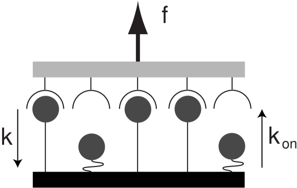
Figure 1: Schematic representation of an adhesion cluster under constant shared force: there are $N_{t}=5$ receptor-ligand pairs, $i=3$ of which are closed and equally share the load $f$. A closed bond ruptures with the dissociation rate $k=k_{0}e^{f/i}$. The $N_{t}-i=2$ open bonds rebind with the force-independent association rate $k_{on}$. Our model has three parameters: cluster size $N_{t}$, dimensionless rebinding rate $\gamma=k_{on}/k_{0}$ and dimensionless force $f$.

The rupture of molecular bonds can be modelled in the framework of Kramers theory as thermally activated escape over a transition state barrier Evans and Ritchie (1997); Izrailev et al. (1997); Shillcock and Seifert (1998). Assuming an infinitely sharp transition state barrier leads to the so-called Bell equation for the single molecule dissociation rate as a function of force, $k=k_{0}e^{F/F_{b}}$ Bell (1978). Here the force scale $F_{b}=k_{B}T/x_{b}$ is set by thermal energy $k_{B}T$ and the distance $x_{b}$ between the potential minimum and the transition state barrier along the reaction coordinate of rupture. For a typical value $x_{b}\simeq 1$ nm and physiological temperature $T\simeq 300$ K, we find the typical force scale $F_{b}\simeq 4$ pN. Physiological loading has indeed been found to be in the pN-range, both for cell-matrix adhesion Balaban et al. (2001); Schwarz et al. (2002); Tan et al. (2003) and rolling adhesion Alon et al. (1995, 1997). Values for $k_{0}$ and $F_{b}$ have been measured during recent years with dynamic force spectroscopy for different receptor-ligand systems, including integrins Zhang et al. (2002); Li et al. (2003), cadherins Baumgartner et al. (2000) and selectins Fritz et al. (1998); Evans et al. (2001). While the dissociation rate $k$ depends mainly on the internal structure of a bond, the association rate $k_{on}$ includes the formation of an encouter complex and therefore depends on the details of the situation under consideration. It is very difficult to determine $k_{on}$ experimentally, especially in the case of cell adhesion, when the interacting molecules are anchored to opposing surfaces Chesla et al. (1998); Zhu (2000); Orsello et al. (2001). In order to focus on the generic features of cluster stability, here we assume that $k_{on}$ is a force-independent constant, in accordance with earlier theoretical work Bell (1978); Hammer and Lauffenburger (1987); Cozens-Roberts et al. (1990); Seifert (2000). Future modelling might refine this assumption, considering for example the effect of ligand-receptor separation controlled by polymeric tethers Jeppesen et al. (2001); Moreira et al. (2003); Moreira and Marques (2004).

For the following, it is convenient to use dimensionless quantities. We define dimensionless time $\tau=k_{0}t$, dimensionless force $f=F/F_{b}$ and dimensionless rebinding rate $\gamma=k_{on}/k_{0}$. The dimensionless single molecule dissociation rate is $k/k_{0}=e^{f}$. We consider a cluster with a constant number of $N_{t}$ bonds, which initially are all closed and then undergo rupture and rebinding according to the appropriate rates. Since bond rupture is a discrete process, the stochastic dynamics of the bond cluster can be described by the one-step master equation van Kampen (1992)

$$\frac{dp_{i}}{d\tau}=r_{i+1}p_{i+1}+g_{i-1}p_{i-1}-[r_{i}+g_{i}]p_{i}\ ,$$ (1)

where $p_{i}(\tau)$ is the probability that $i$ bonds are closed at time $\tau$. Here the $r_{i}$ and $g_{i}$ are the reverse and forward rates between the possible states $i$ ($0\leq i\leq N_{t}$). They follow from dissociation and association rates of single bonds as

$$r_{i}=r(i)=ie^{f/i}\quad\text{and}\quad g_{i}=g(i)=\gamma(N_{t}-i)\ .$$ (2)

Our model has three parameters, namely cluster size $N_{t}$, rebinding rate $\gamma$ and force $f$. Since $i\geq 0$ should be guaranteed at any time, $r_{0}=0$ has to be set for $f>0$, in addition to the definitions in Eq. (2). Moreover, Eq. (2) implies $g_{0}>0$, that is, after rupture of the last closed bond new bonds are allowed to form. This corresponds to a reflecting boundary of the master equation at $i=0$. As explained above, in biological and biomimetic situations rebinding of the completely dissociated state is usually prevented by elastic recoil of the transducer. Therefore in the following we set $g_{0}=0$ in order to model an absorbing boundary at $i=0$. Because the values for $r_{0}$ and $g_{0}$ do not follow the general form given in Eq. (2), the boundary at $i=0$ is an artificial boundary. Concerning the upper end of the set of states at $i=N_{t}$, the form $g_{N_{t}}=0$ represents a reflecting boundary and guarantees $i\leq N_{t}$. Thus, the upper boundary is a natural boundary of the master equation.

A quantity of large interest is the average number of closed bonds $N(\tau)=\langle i\rangle=\sum_{i=1}^{N_{t}}ip_{i}(\tau)$. From the master equation Eq. (1) one can derive Honerkamp (1990)

$$\frac{dN}{d\tau}=\sum_{i=0}^{N_{t}}i\frac{dp_{i}}{d\tau}=-\langle r(i)\rangle+\langle g(i)\rangle\ .$$ (3)

If $r(i)$ and $g(i)$ were both linear functions in $i$, Eq. (3) would become an ordinary differential equation for $N$. This suggests to study the deterministic equation

$$\frac{dN}{d\tau}=-r(\langle i\rangle)+g(\langle i\rangle)=-Ne^{f/N}+\gamma(N_{t}-N)$$ (4)

as has been done by Bell Bell (1978). Below we will see that the analysis of this equation gives valuable insight into the generic features of our model. However, it is important to note that for $f>0$, the reverse rate $r(i)$ in Eq. (2) is non-linear in $i$ and the average in Eq. (3) cannot be taken. Instead lower moments are related to higher moments and one arrives at a complicated hierarchy of coupled differential equations. The solution of the deterministic equation Eq. (4) will therefore deviate from the average number of closed bonds obtained from the solution of the master equation Eq. (1). The same problem arises for the higher moments. For example, for the variance $\sigma_{N}^{2}=\langle i^{2}\rangle-\langle i\rangle^{2}$ one can derive Honerkamp (1990)

$$\frac{d\sigma_{N}^{2}}{dt}=\langle g(i)+r(i)\rangle\ +2\langle(i-\langle i\rangle)(g(i)-r(i))\rangle\ ,$$ (5)

where again the average cannot be taken. As an approximate treatment, one can expand $r(i)$ in a Taylor series around the average for $i$, $\langle i\rangle=N$ van Kampen (1992). Restricting the expansion to second order, thus assuming a Gaussian distribution, leads to the following equations

$$\frac{dN}{d\tau} =-Ne^{f/N}+\gamma(N_{t}-N)-\sigma_{N}^{2}e^{f/N}\frac{f^{2}}{2N^{3}}\ ,$$ (6)

$$\frac{d\sigma_{N}^{2}}{d\tau} =Ne^{f/N}+\gamma(N_{t}-N)-\sigma_{N}^{2}\left(e^{f/N}\left(2-\frac{2f}{N}-\frac{f^{2}}{2N^{3}}\right)+\gamma\right)\ .$$ (7)

In principle, these equations can be solved by numerical integration. However, it is much more instructive to consider the original master equation. Moreover, the deterministic equation Eq. (4) and its improved version Eq. (6) cannot describe the effect of an absorbing boundary at $i=0$. In order to consider this experimentally relevant case, one has to study the master equation Eq. (1) with the rates given in Eq. (2). Finally, only the full stochastic analysis reveals the detailed effect of fluctuations.

II.2 Numerical solution

Below we will present analytical solutions for several special cases of the master equation. In the general case, we numerically solve the master equation by Monte Carlo methods. In detail, for each set of parameter values $N_{t}$, $f$ and $\gamma$, we generate between $10^{4}$ and $10^{6}$ trajectories with the help of the Gillespie algorithm for exact stochastic simulations Gillespie (1976, 1977). By averaging for given time $\tau$ over the different simulation trajectories, we obtain the desired probability distributions $\{p_{i}(\tau)\}_{i=0}^{N_{t}}$. In general it is also rather instructive to study single simulation trajectories, because their specific features are expected to be characteristic also for experimental trajectories.

The Gillespie algorithm was originally developed for exact simulation of the stochastic dynamics of coupled chemical reactions. Applied to our case, open and closed bonds correspond to two different species of molecules and the transition between these two species, that is rupture and rebinding, correspond to chemical reactions. The Gillespie algorithm is very efficient because rather than discretizing time in small steps, it generates jumps between subsequent reactions. The basic quantity of the Gillespie algorithm is the probability $P(\mu,\tau|\tau_{0},X)d\tau$ that the next reaction occurs in the time interval $[\tau_{0}+\tau,\tau_{0}+\tau+d\tau]$ and is of type $\mu$ under the condition that at time $\tau_{0}$ the system is in state $X$. In our case, $\mu$ has only two values corresponding to rupture and rebinding, and the state $X$ of the system is completely described by the number of closed bonds $i$. Since the rupture and rebinding rates from Eq. (2) are constant between subsequent events, $P$ does not depend on absolute time $\tau_{0}$. In fact it reads

$$P(\mu,\tau|\tau_{0},X)=P(\mu,\tau|i)=P_{0}(\tau|i)a_{\mu}$$ (8)

where $P_{0}$ is the probability that no reaction occurs in the time interval $[0,\tau]$ and $a_{\mu}$ is the reaction rate for reaction $\mu$. $P_{0}$ satisfies the differential equation

$$\frac{dP_{0}}{d\tau}=-\left(\sum_{\mu}a_{\mu}\right)P_{0}\ ,$$ (9)

and the initial condition $P_{0}(0)=1$, therefore $P_{0}(\tau|i)=e^{-\left(\sum_{\mu}a_{\mu}\right)\tau}$. $P(\mu,\tau|i)$ is properly normalised to unity as can be shown by integrating over time and summing over reactions. The Gillespie algorithm generates trajectories in which subsequent reactions are separated by the following rule. In the absence of other reactions, the probability for a reaction $\mu$ in the time interval $[\tau,\tau+d\tau]$ is given by

$$p_{\mu}(\tau)=a_{\mu}e^{-a_{\mu}\tau}d\tau\ .$$ (10)

The integral

$$F_{\mu}(\tau)=\int_{0}^{\tau}p_{\mu}(\tau^{\prime})d\tau^{\prime}=1-e^{-a_{\mu}\tau}$$ (11)

is the probability for a reaction occuring until time $\tau$. It increases strictly monotonically from $0$ to unity and thus can be inverted. In order to generate a random variable $\tau_{\mu}$ which is distributed according to Eq. (10), one generates a random number $\xi$ which is uniformly distributed over the interval $[0,1]$ and inserts it into the formula

$$\tau_{\mu}=-\frac{\ln(\xi)}{a_{\mu}}\ .$$ (12)

This is done for each type of reaction, leading to a set of times $\tau_{\mu}$. The time for the next reaction is then chosen as the smallest $\tau_{\mu}$, that is $\tau=\min_{\mu}(\tau_{\mu})$. As shown in Gillespie (1976, 1977), this rule generates trajectories with the correct distribution of times and types of subsequent reactions. With the forward and reverse rates Eq. (2) for rebinding and unbinding of molecular bonds in the cluster, the random times are determined by the functions

$$\tau_{f}=-\frac{\ln(\xi)}{\gamma(N_{t}-i)}\quad\text{and}\quad\tau_{r}=-\frac{\ln(\xi)}{ie^{f/i}}\ .$$ (13)

This algorithm is exact in the sense that the only sources of inaccuracy lie in the choice of the random number generator and the finite number of trajectories used to calculate probability distribution.

III Vanishing rebinding

III.1 Deterministic analysis

We start our analysis with the case of vanishing rebinding, $\gamma=0$. Then the deterministic equation Eq. (4) reads

$$\frac{dN}{d\tau}=-Ne^{f/N}\ .$$ (14)

In principle, the total number of bonds $N_{t}$ is irrelevant in this case. However, it is reintroduced through the initial condition $N(0)=N_{t}$. Then Eq. (14) is solved implicitly by Bell (1978)

$$\tau\left(N\right)=E\left(\frac{f}{N_{t}}\right)-E\left(\frac{f}{N}\right)$$ (15)

where $E(z)=\int_{z}^{\infty}dz^{\prime}e^{-z^{\prime}}/z^{\prime}$ is the exponential integral. Unfortunately, the inversion for $N(\tau)$ is not possible in general.

In the deterministic description, cluster lifetime $T_{det}$ can be identified with the time $\tau$ at which only one last bond exists. Setting $N(T_{det})=1$ in Eq. (15) gives

$$T_{det}=E\left(\frac{f}{N_{t}}\right)-E\left(f\right)\ .$$ (16)

From this result, we can extract three different scaling regimes. For small force, $f<1$, we use the small argument expansion of the exponential integral, $E(z)\approx-\Gamma-\ln(z)$ (where $\Gamma=0.577$ is the Euler constant), and find

$$T_{det}\approx\ln N_{t}\ .$$ (17)

This corresponds to the familiar case of radioactive decay, when the differential equation $dN/d\tau=-N$ leads to exponential decay $N=N_{t}e^{-\tau}$.

For intermediate force, $1<f<N_{t}$, we can rewrite Eq. (16) for the cluster lifetime as the sum of two integrals,

$$T_{det}=\int_{f/N_{t}}^{1}dz\frac{e^{-z}}{z}+\int_{1}^{f}dz\frac{e^{-z}}{z}\ .$$ (18)

The second integral can be estimated to be $\int_{1}^{f}dz(e^{-z}/z)<\int_{1}^{f}dze^{-z}=e^{-1}-e^{-f}<e^{-1}$. For the first integral, we can expand the integrand for small arguments, leading to $\int_{f/N_{t}}^{1}dz(e^{-z}/z)\approx\int_{f/N_{t}}^{1}dz(1-z)/z\approx\ln(N_{t}/f)$. Since $N_{t}>f$, the second integral can be neglected and we have

$$T_{det}\approx\ln\left(\frac{N_{t}}{f}\right)\ .$$ (19)

For the time evolution of the cluster, both exponential integrals in Eq. (15) can be replaced by the small argument approximation as long as $N>f$ and hence the exponential decay proceeds until the force per bond is $f/N=1$. Thereafter the decay will be faster than exponential due to the destabilizing effect of force.

For large force, $f>N_{t}$, the second term in Eq. (16) can be neglected and we can use the large argument approximation for the exponential integral, $E(z)\approx e^{-z}/(1+z)$, leading to Bell (1978)

$$T_{det}\approx\frac{e^{-f/N_{t}}}{1+f/N_{t}}\quad.$$ (20)

Therefore cluster lifetime decays faster than exponential with $f/N_{t}$ in this regime. Now the small argument approximation is not applicable to either of the two terms in Eq. (15) and the decrease in $N$ will be faster than exponential over the whole range of time.

In summary, the analysis of the deterministic equation Eq. (14) allows to identify three scaling regimes of small, intermediate and large force. This analysis also shows that $f/N_{t}$ is an important scaling variable, which we will therefore use to analyse also the stochastic case.

III.2 Stochastic analysis

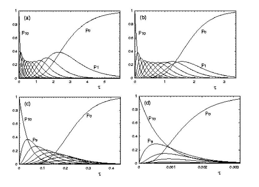
Figure 2: The state probability $p_{i}(\tau)$ is the probability that $i$ bonds are closed at time $\tau$ ($0\leq i\leq N_{t}$). Here the $p_{i}$ are plotted as a function of time $\tau$ for a cluster of initial size $N_{t}=10$ for $\gamma=0$ and (a) $f=0$, (b) $f=1$, (c) $f=10$ and (d) $f=50$.

For finite force, $f>0$, the reverse rate $r(i)$ in Eq. (2) is non-linear in $i$ and the boundary at $i=0$ is artificial. Therefore the master equation in general cannot be solved with standard techniques. However, in the case of vanishing rebinding, $\gamma=0$, one can use the fact that the decay of the cluster corresponds to a unique sequence of events, with the number of closed bonds decreasing monotonously from $N_{t}$ to $0$. The transition from state $i$ (with $i$ closed bonds present) to the state $i-1$ (with one more broken bond) is a Poisson process with the time-independent rate $r_{i}$. If $i$ bonds are present at time $\tau$, the probability that the next bond ruptures at time $\tau+\tau^{\prime}$ is given by

$$p_{i\to i-1}(\tau^{\prime})=r_{i}e^{-r_{i}\tau^{\prime}}\ .$$ (21)

The state probability $p_{i-1}$ is related to the state probability $p_{i}$ and the transition probability $p_{i\to i-1}$ by the recursive expression

$$p_{i-1}(\tau)=\int_{0}^{\tau}d\tau^{\prime}\ p_{i}(\tau^{\prime})p_{i\to i-1}(\tau-\tau^{\prime})=r_{i}e^{-r_{i}\tau}\int_{0}^{\tau}d\tau^{\prime}\ p_{i}(\tau^{\prime})e^{r_{i}\tau^{\prime}}\ ,$$ (22)

which uses the fact that the state $i-1$ can be reached only through the state $i$. This scheme is solved by

$$p_{i}(\tau)=\left(\prod_{j=i+1}^{N_{t}}r(j)\right)\sum_{j=i}^{N_{t}}\left\{e^{-r(j)\tau}\prod_{\begin{subarray}{c}k=i\\ k\neq j\end{subarray}}^{N_{t}}\frac{1}{r(k)-r(j)}\right\}$$ (23)

as can be shown by induction. The properties of this expression follow from the properties of the reverse rate $r(i)=ie^{f/i}$, which for finite force, $f>0$, is a non-monotonous function of $i$. It diverges for $i\to 0$, has a minimum at $i=[f]$ (the integer closest to $f$) and grows as $i$ for $i\to\infty$. In the unlikely case that the value of $f$ is such that $r(j)=r(k)$ for $j\neq k$, the limit of the expression in Eq. (23) for $r(k)\to r(j)$ has to be taken carefully. In order to treat this case properly, one has to replace Eq. (23) by

$$p_{i}(\tau)=\left(\prod_{j=i+1}^{N_{t}}r(j)\right)\sum_{j=i}^{N_{t}}\left\{e^{-r(j)\tau}\left(\prod_{\begin{subarray}{c}k=i\\ r(k)\neq r(j)\end{subarray}}^{N_{t}}\frac{1}{r(k)-r(j)}\right)\left(\prod_{\begin{subarray}{c}k=i\\ r(k)=r(j)\\ k\neq j\end{subarray}}^{N_{t}}\frac{\tau}{2}\right)\right\}\ ,$$ (24)

where we have used $\lim_{\Delta\to 0}(1-e^{-\Delta\tau})/\Delta=\tau$ for $\Delta=r(i)-r(k)$. In Fig. 2 we plot the full solution to the master equation, that is the state probabilities $p_{i}(\tau)$ from Eq. (23), for $N_{t}=10$ and four different values of force $f$. For small force, all states are appreciably occupied during the decay, that is each of the curves is a maximum of the set of curves during a certain period of time. In the long run, $p_{0}$ approaches unity and all other $p_{i}$ disappear, because without rebinding, the cluster has to dissociate eventually. For increasing force, the shape of the curves changes considerably. Now the lower states (with small number of closed bonds $i$) hardly become occupied during the decay process. For very large force, the maximum occupancy changes directly from the initial state $N_{t}$ over to the detached state $0$.

Figure 3: Average number of closed bonds $N$ as a function of time $\tau$ for different cluster sizes $N_{t}=1,2,4,8$ and $16$. (a) $f/N_{t}=0.01$, (b) $f/N_{t}=0.1$, (c) $f/N_{t}=1.0$ and (d) $f/N_{t}=5.0$.

With the help of the exact solution Eq. (23), any quantitiy of interest can now be calculated. One quantity of large interest is the average number $N(\tau)=\langle i\rangle=\sum_{i=1}^{N_{t}}ip_{i}(\tau)$ of closed bonds at time $\tau$. For a single bond, $N$ is simply the probability $p_{1}$ that the bond is attached,

$$N(\tau)=p_{1}(\tau)=e^{-e^{f}\tau}\ .$$ (25)

For a two-bond cluster we have

$$N(\tau)=p_{1}(\tau)+2p_{2}(\tau)=\frac{2}{2-e^{f/2}}\left\{e^{-e^{f}\tau}+(1-e^{f/2})e^{-2e^{f/2}\tau}\right\}\ .$$ (26)

For increasing $N_{t}$, the corresponding expressions become increasingly cumbersome. In general, $N(t)$ is a sum of $N_{t}$ exponentials with the different relaxation rates $r(i)$ with $1\leq i\leq N_{t}$. For small force, $f<1$, $r(i)\approx i$ and the smallest rate corresponds to $i=1$, that is, $N\sim e^{-\tau}$ on large time scales. In this case, clusters of any size decay with the same slope as single bonds and the difference between single and multiple bond rupture lies in the prefactor, not in the time-scale of average decay. For intermediate force, $1<f<N_{t}$, and large time scales, decay is dominated by $i=[f]$, that is $N\sim e^{-fe\tau}$. Thus the absolute value of force governs the long time behavior, with different sizes showing up only in the prefactor. For large force, $f>N_{t}$, decay at large time scales is dominated by $i=N_{t}$, that is $N\sim e^{-N_{t}e^{f/N_{t}}\tau}$. This implies that for a given force $f$, the largest clusters show the slowest decays in the long run. However, if one controls $f/N_{t}$ rather than $f$, the cluster with the smallest size will decay the slowest, since it is subject to the smallest absolute force. In Fig. 3 we plot $\log N$ as a function of time $\tau$ for different values of cluster size $N_{t}$ and force per initial bond, $f/N_{t}$. All curves initially show an exponential decay with the rate of a single bond. For small forces decay stays exponential for almost all times. The larger force, the earlier decay crosses over to the late stage regime of super-exponential decay.

Figure 4: Average number of closed bonds $N$ as a function of time $\tau$ for $N_{t}=8$ and $16$ and (a) $f/N_{t}=0.1$ and (b) $f/N_{t}=1$. Solid and dashed lines are stochastic and deterministic results, respectively.

As noted in Sec. II, due to the non-linear form of $r(i)=ie^{f/i}$ for $f>0$, the first moment $N(\tau)$ of the stochastic solution Eq. (23) is not identical with the function $N(\tau)$ obtainted from the deterministic equation Eq. (14). In Fig. 4, results for $N(\tau)$ derived from the deterministic and the stochastic description are compared to each other. For a small but non-zero force, the non-linearity is small and the agreement between the two results is good in the initial phase of the decay. Towards the end of the decay strong deviations are observed. Here, the force on each bond grows strongly and the non-linearity of the transition rates is large. For increasing force, fluctuations become less relevant and the deviation between deterministic and stochastic results is increasingly restricted to the very end of the decay process.

Figure 5: Single simulation trajectories (solid lines) compared with the average number of closed bonds $N(\tau)$ (dashed lines) for $N_{t}=10$ and $25$ and (a) $f/N_{t}=0.1$ and (b) $f/N_{t}=1$. In (b), in addition the deterministic results are plotted as dotted lines.

In Fig. 5a and b the result for the mean number of closed bonds $N(\tau)$ is compared to single simulation trajectories for small and large forces, respectively. The single simulation trajectories are expected to resemble experimental realizations for the time evolution of the number of closed bonds. The figure shows that for small force, the trajectories decay in a similar way as does the average. For large force, the trajectories decay in a more abrupt way than the averages, that is they appear to run along the average for most of the time, but then decay rather abruptly towards the completely dissociated state. In this case, fluctuations do not so much affect the typical shape of the rupture trajectory, but rather the timepoint of rupture. The reason for this typical behavior is that a large fluctuation towards the absorbing boundary inevitably leads to a runaway process, since force is increasingly focused on less and less bonds due to shared loading. This type of rupture process is similar to avalanches or cascading failures in highly connected systems. Although rupture is rather abrupt, its timepoint is widely distributed, leading to the smooth decrease of $N(\tau)$ observed in the average. In the large force case in Fig. 5b, we also show the deterministic results for $N(\tau)$ (for the small force case in Fig. 5a, they hardly differ from the stochastic results). These curves show that the abrupt decay of single simulation trajectories at large force is somehow predicted by the deterministic description, compare Fig. 4. This had to be expected because the deterministic equation describes a representative yet single trajectory.

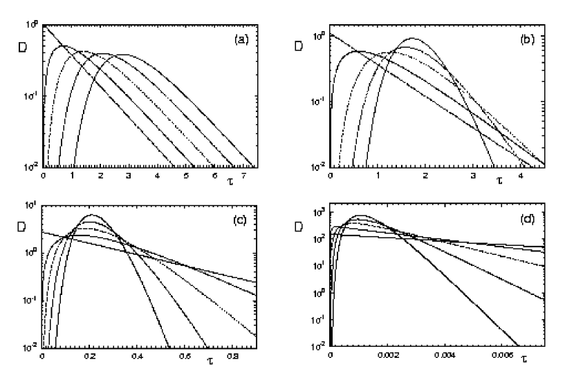
Figure 6: Probability for dissociation of the whole cluster $D$ as a function of time $\tau$ for $N_{t}=1,2,4,8$ and $16$ for (a) $f/N_{t}=0.0$, (b) $0.1$, (c) $1.0$ and (d) $5.0$.

The probability for dissociation of the overall cluster (that is for rupture of the last bond) is defined by $D(\tau)=\dot{p}_{0}(\tau)=r_{1}p_{1}(\tau)$ and follows from Eq. (23) with the reverse rate $r_{1}$ from Eq. (2). The resulting formula has been given before in Ref. Tees et al. (2001). For a single bond it is simply $D(\tau)=e^{f}e^{-e^{f}\tau}$. For $N_{t}=2$ we have

$$D(\tau)=\frac{2e^{f}}{2-e^{f/2}}\left(e^{-e^{f}\tau}-e^{-2e^{f/2}\tau}\right)\ .$$ (27)

In the special case $f=2\ln 2$, the two rates $r(1)$ and $r(2)$ are equal and we have

$$D(\tau)=16\tau e^{-4\tau}\ .$$ (28)

In general, as for $N(\tau)$, $D(\tau)$ is a sum of exponentials $e^{-r(i)\tau}$ and the decrease on long time scales is governed by the exponential which decreases the slowest. In Fig. 6 we plot $D(\tau)$ for different values of $N_{t}$ and $f/N_{t}$ (by controlling $f/N_{t}$ rather than $f$, the curves have comparable averages). The case $N_{t}=1$ is a Poisson process with simple exponential decay. For $N_{t}>1$, $D(0)=0$, because instantaneous rupture of all bonds at $\tau=0$ is a higher order process. For large times, all curves decay exponentially. For vanishing force, $f=0$, the curves are very similar, with the same slope at large times. The maxima of the cluster dissociation rates for $f=0$ are described by $T_{max}=\ln N_{t}$, in agreement with the result Eq. (17) from the deterministic description. For small $f/N_{t}$, the distributions are Gauss-like with small asymmetry and variance. For large $f/N_{t}$, they became Poisson-like, that is they develop a strong asymmetry with a maximum close to zero and a pronounced long-time tail. The reason is that in this case, decay is dominated by rupture of the first bond, that is we are effectively back to a single bond system (except that $D(0)=0$ as always for multiple bonds).

Figure 7: Average adhesion cluster lifetime $T$ as a function of $f/N_{t}$ for cluster sizes $N_{t}=1,10,100,1000$ and $10000$. The dashed horizontal curves are the harmonic numbers, which are good approximations in the small force regime, $f<1$. The dotted curve is the approximation $T=\ln\left(0.61N_{t}/f\right)$ for the intermediate force regime, $1<f<N_{t}$.

The average cluster lifetime can in principle be calculated as the first moment of the overall dissociation rate

$$T=\int_{0}^{\infty}d\tau\ \tau\ D(\tau)\ .$$ (29)

In practice, it has a simple form which can be derived without using the probability distribution Eq. (23). The waiting time spent in state $i$ before the transition into state $i-1$ is a stochastic variable characterised by the distribution function Eq. (21). Its average is given by the inverse transition rate $1/r(i)$. Since the decay process is a sequence of such independent Poisson processes, we simply have

$$T=\sum_{i=1}^{N_{t}}\frac{1}{r(i)}\ .$$ (30)

For $f=0$ we get Goldstein and Wofsy (1996); Tees et al. (2001)

$$T=\sum_{i=1}^{N_{t}}\frac{1}{i}=H_{N_{t}}$$ (31)

which are the harmonic numbers. The lifetime of a two-bond cluster is increased by a factor $3/2=1.5$ with respect to the single bond, that of the three-bond cluster by $11/6=1.8$, and so on. For large $N_{t}$ one can write Goldstein and Wofsy (1996)

$$T\approx\ln N_{t}+\frac{1}{2N_{t}}+\Gamma$$ (32)

where $\Gamma=0.577$ is the Euler constant. In fact this approximation is very good already for small values of $N_{t}$. The weak (logarithmic) dependence for large $N_{t}$ means that for large adhesion clusters, size matters little since the bonds decay independently of each other and on the same time-scale. This result differs from the deterministic one for small force, Eq. (17), by the constant $\Gamma$ and the additional contribution $1/2N_{t}$, which vanishes for large clusters. For small force, $f<1$, Eq. (32) is a good approximation for cluster lifetime $T$. For intermediate force, $1<f<N_{t}$, the reverse rate grows rapidly for states with $i<f$, whereas for states with $i>f$, $r(i)$ remains close to $i$. Therefore we can approximate the average lifetime of a cluster as $H_{N_{t}}-H_{f}$. Using Eq. (32), we get

$$T\simeq\ln\left(N_{t}/f\right)\ .$$ (33)

Thus cluster size $N_{t}$ is now replaced by an effective size $N_{t}/f$, as we have already found in the deterministic framework, compare Eq. (19). For large force, $f>N_{t}$, the only term which contributes to Eq. (30) is the one for the rupture of the first bond. Then

$$T\approx\frac{e^{-f/N_{t}}}{N_{t}}$$ (34)

and we deal essentially with a single bond effect: if the first bond breaks, all remaining bonds follow within no time (‘domino effect’). This effect is also evident from the dissociation rate $D(\tau)$, which for very large force approaches a Poisson distribution, compare Fig. 6d. In Eq. (34), the numerator represents the probability for single bond rupture under force, while the denominator represents the probability that any one out of $N_{t}$ identical bonds breaks first. Since $f>N_{t}$ in this regime, the first effect dominates and $T$ increases with $N_{t}$. For a given $f/N_{t}$, on the other hand, the lifetime decreases with increasing $N_{t}$, due to the increase in absolute force. In contrast to the deterministic result, Eq. (20), the stochastic result Eq. (34) does not scale with $f/N_{t}$. In Fig. 7 we plot the average cluster lifetime $T$ from Eq. (30) as a function of $f/N_{t}$ for different values of $N_{t}$. For small force, $f<1$, $T$ plateaus at the value given by the harmonic number $H_{N_{t}}$ according to Eq. (31). In the regime of intermediate force, $1<f<N_{t}$, all curves fall on the master curve $T=\ln\left(0.61(N_{t}/f)\right)$, as predicted by Eq. (33). For large force, $f>N_{t}$, the scaling with $f/N_{t}$ is lost, as predicted by Eq. (34). Although deterministic and stochastic predictions for cluster lifetime $T$ have similar overall features, the deterministic result underestimates the plateau at small force and predicts an incorrect scaling with $f/N_{t}$ at large force.

Figure 8: (a) Variance $\sigma_{N}$ for the number of closed bonds in relation to the average number of closed bonds $N$ as function of time $\tau$ for $f/N_{t}=1.0$ and $N_{t}=8$ (solid) and $16$ (dashed). (b) Variance $\sigma_{T}$ for cluster lifetime in relation to average cluster lifetime $T$ as a function of $f/N_{t}$ for $N_{t}=1,10,100,1000$ and $10000$.

Higher cumulants of the various distributions provide information about the effect of fluctuations. For the number of closed bonds at time $\tau$, the width of the distribution is described by the variance, defined by $\sigma^{2}_{N}(\tau)=\langle i^{2}\rangle-\langle i\rangle^{2}$. In Fig. 8a, we plot the relative standard deviation, $\sigma_{N}(\tau)/N(\tau)$, for cluster sizes $N_{t}=8$ and $N_{t}=16$. It it zero initially due to the initial condition and diverges for large times. In regard to the distribution of cluster lifetime, the variance $\sigma_{T}$ can be calculated in the same way as the average lifetime, because for a sequence of independent stochastic processes, all cumulants simply add up. The variance of the Poisson process Eq. (21) is $1/r^{2}(i)$. Therefore the variance for cluster lifetime is

$$\sigma^{2}_{T}=\sum_{i=1}^{N_{t}}\frac{1}{r^{2}(i)}\ .$$ (35)

For vanishing force this expression reads

$$\sigma^{2}_{T}=\sum_{i=1}^{N_{t}}\frac{1}{i^{2}}=\zeta(2)-\psi^{(1)}(N_{t}+1)\ ,$$ (36)

where $\psi^{(1)}(N_{t}+1)$ is the trigamma function and $\zeta$ the Riemannian $\zeta$-function. For increasing $N_{t}$, the variance converges to a finite value. For zero force this limit is given by

$$\sigma^{2}_{T}=\sum_{i=1}^{\infty}\frac{1}{i^{2}}=\zeta(2)=\frac{\pi^{2}}{6}\ ,$$ (37)

because the trigamma function vanishes in this limit. This result is an upper limit for the variance in general, because the reverse rate increases with increasing force, $r(i)\geq i$. The relative standard deviation $\sigma_{T}/T$ of cluster dissociation is always smaller than unity, since $(\sum x)^{2}>\sum x^{2}$. For single bond rupture, we have a single Poisson process and it becomes exactly unity. For vanishing force and large clusters, it scales as $\sim 1/\ln N_{t}$. Although it decreases with increasing $N_{T}$, it does so in a different way than the Gauss process, which decreases as $\sim 1/N_{t}^{1/2}$. The reason is that the contributions from the different subprocesses are not constant, but decrease as rupture proceeds. For large forces, $f>N_{t}$, cluster dissociation becomes a Poisson process governed by the rupture of the first bond. Then the first term dominates in Eq. (30) and Eq. (35). Therefore the relative standard deviation $\sigma_{T}/T\approx 1$ again. Moreover, now $\sigma_{T}/T\sim 1/N_{t}^{1/2}$, because now only the first $N_{t}-f$ subprocesses contribute, with roughly similar values, like in a Gauss-distribution. In Fig. 8b, we plot $\sigma_{T}/T$ as a function of $f/N_{t}$ as it crosses over between the cases of vanishing and very large force, with a minimum around $f/N_{t}\approx 0.3$, that is in the intermediate force range. The narrow distribution at intermediate force is also evident in Fig. 6. Fig. 8b also shows how the relative standard deviation decreases with increasing cluster size $N_{t}$. In general, the agreement between deterministic and stochastic descriptions is best for large cluster size $N_{t}$ and intermediate force $1<f<N_{t}$. However, it should also be noted that the definition of deterministic lifetime is somehow arbitrary, because a discrete cutoff has to be introduced in a continuum description. Especially for small clusters the choice of the cluster size at which dissociation occurs will have a large influence on $T$.

IV Vanishing force

IV.1 Deterministic analysis

We now turn to the case of vanishing force, $f=0$. Then the deterministic equation Eq. (4) reads

$$\frac{dN}{d\tau}=-N+\gamma(N_{t}-N)\ .$$ (38)

For the initial condition $N(0)=N_{t}$, its solution is

$$N(\tau)=\frac{\gamma+e^{-(1+\gamma)\tau}}{1+\gamma}N_{t}=\left[1+\frac{1}{\gamma}e^{-(1+\gamma)\tau}\right]N_{eq}\ .$$ (39)

Thus there is an exponentially fast relaxation from $N_{t}$ to the equilibrium state with $N_{eq}=\gamma N_{t}/(1+\gamma)$ closed bonds. $N_{eq}$ increases linearly with the rebinding constant $\gamma$ from $N_{eq}=0$ for $\gamma=0$ and saturates at $N_{t}$ for $\gamma>1$. In the deterministic description, the lifetime of the cluster is infinite, because the completely dissociated state $N=0$ is never reached.

IV.2 Stochastic analysis

In the case $f=0$, the reverse rates defined in Eq. (2) are linear in $i$ and $r(0)=0$ at $i=0$. Natural boundary conditions imply $g(0)=\gamma N_{t}$, that is a reflecting boundary condition at $i=0$. A linear system with natural boundary conditions can be solved with standard techniques. For the initial condition $p_{i}(0)=\delta_{i,N_{t}}$, a generating function has been derived by Mc Quarrie McQuarrie (1963):

$$G(s,\tau)=\sum_{i=0}^{N_{t}}s^{i}p_{i}(\tau)=\left(\frac{(s-1)e^{-(1+\gamma)\tau}+1+\gamma s}{(1+\gamma)}\right)^{N_{t}}\ .$$ (40)

The state probabilities follow from the generating function as

$$p_{i}(\tau)=\frac{1}{i!}\left.\frac{\partial^{i}G(s,\tau)}{\partial s^{i}}\right|_{s=0}=\binom{N_{t}}{i}\frac{\left(\gamma+e^{-(1+\gamma)\tau}\right)^{i}\left(1-e^{-(1+\gamma)\tau}\right)^{N_{t}-i}}{(1+\gamma)^{N_{t}}}\ .$$ (41)

One can easily check that by setting $\gamma=0$ in Eq. (41), one obtains the same result as by setting $f=0$ in Eq. (23). Eq. (41) shows that the systems relaxes to the stationary state on a dimensionless time scale $1/(1+\gamma)$, thus the larger rebinding, the faster the system equilibrates. In the stationary state, the state probabilities follow a binomial distribution

$$p_{i}(\infty)=\binom{N_{t}}{i}\frac{\gamma^{i}}{(1+\gamma)^{N_{t}}}$$ (42)

because the bonds are independent and each bond is closed and open with probabilities $\gamma/(1+\gamma)$ and $1/(1+\gamma)$, respectively.

The generating function also allows to calculate all moments of the distribution:

$$\langle i^{n}\rangle=\left.\frac{\partial^{n}G(s,\tau)}{\partial(\ln s)^{n}}\right|_{s=1}\quad.$$ (43)

Since now $r(i)$ is linear in $i$, the first moment $N(\tau)=\langle i\rangle$ is identical to the solution Eq. (39) of the deterministic equation. In order to assess the role of fluctuations, we calculate the variance:

$$\sigma^{2}_{N}(\tau)=\langle i^{2}\rangle-\langle i\rangle^{2}=\frac{(1-e^{-(1+\gamma)\tau})}{(1+\gamma)}N(\tau)\ .$$ (44)

The relative standard deviation $\sigma_{N}/N$ essentially scales as $N^{-1/2}$ for all times, thus fluctuation effects decrease with increasing bond number in the usual way. The stationary state value is $\lim_{\tau\to\infty}\sigma_{N}(\tau)/N(\tau)=((1+\gamma)N_{eq})^{-1/2}=(\gamma N_{t})^{-1/2}$. Therefore larger rebinding does not only increase the equilibrium number of bonds, but also decreases the size of the fluctuations around $N_{eq}$. This leads to a narrow distribution for large cluster under strong rebinding, with a small probability of coming close to the lower boundary.

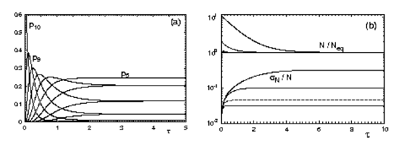
Figure 9: (a) State probabilities $p_{i}(\tau)$ from Eq. (41) for $N_{t}=10$ with $f=0$ and $\gamma=1$ for a reflecting boundary at $i=0$. (b) $N/N_{eq}$ and $\sigma_{N}/N$ for $N_{t}=100$, $f=0$ and $\gamma=0.1$, $1$, $5$ and $10$.

In Fig. 9a, we plot the state probabilities $p_{i}$ from Eq. (41) for cluster size $N_{t}=10$ and rebinding constant $\gamma=1$. The system quickly relaxes to the equilibrium state. The only difference for different initial conditions is in the initial transient. In particular, for $N_{0}=N_{eq}$, the average does not change in time, although the distribution initially spreads to the binomial one. For $\gamma=1$, the stationary distribution is symmetric around the average. The width of the distribution for different $\gamma$ is illustrated in Fig. 9b, which shows the average number of closed bonds normalised by the equilibrium number of bonds, that is $N/N_{eq}$, together with the relative standard deviation, $\sigma_{N}/N$, for different values of the rebinding constant $\gamma$. The curves for $N$ are independent of $N_{t}$ due to the normalization. Fig. 9b shows that with increasing $\gamma$, relaxation becomes faster and the width of the distribution decreases.

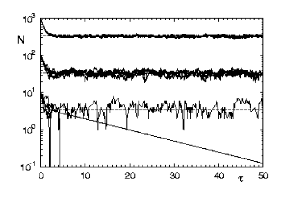
Figure 10: Single simulation trajectories for $f=0$, $\gamma=0.5$, $N_{t}=10,100$ and $1000$ and an absorbing boundary at $i=0$. Solid lines are the average number of closed bonds $N$ and dashed lines are the equilibrium number of closed bonds $N_{eq}$.

For the biologically important case of an absorbing boundary at $i=0$, it seems to be rather difficult to find a closed-form analytical solution for arbitrary cluster sizes. For the case $N_{t}=2$, we will present such a solution in the next section. For arbitrary $N_{t}$, we use Monte Carlo simulations as described in Sec. II. In Fig. 10, we show individual simulation trajectories for different parameter values of interest, in comparision to the average number of closed bonds for reflecting and absorbing boundaries at $i=0$. The plots show that the number of closed bonds in a cluster first relaxes towards the steady state value, for which rupture and rebinding balance each other. Although for the absorbing boundary the number of closed bonds decreases with time in average, for individual realizations it stays roughly constant, until a large fluctuation towards the absorbing boundary leads to loss of this realization. The time-scale for the decrease in $N$ is thus determined by the probability for fluctuations from the steady state to the absorbing boundary.

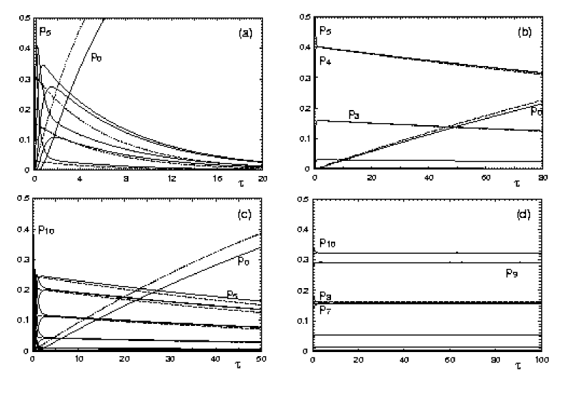
Figure 11: State probabilities $p_{i}$ as a function of time $\tau$ for different cluster sizes $N_{t}=5$ (a and b) and $N_{t}=10$ (c and d) and for rebinding rates $\gamma=1.0$ (a and c) and $5.0$ (b and d). The numerical solutions (solid curves) are compared to the leakage approximation Eq. (46) (dashed curves).

Because a full analytical solution is not available for the case of an absorbing boundary, we now introduce an approximation for this case. It is similar to the local thermal equilibrium description introduced by Zwanzig for modelling protein folding dynamics Zwanzig (1995). Our starting point is that for large clusters and strong rebinding, the absorbing boundary is a small perturbation to the solution for the reflecting boundary, Eq. (41), which in the following we will denote by $\{\bar{p}_{i}\}_{i=0}^{N_{t}}$. Since $g(0)=0$ for the absorbing boundary, $\dot{p}_{0}=r_{1}p_{1}$ with $r_{1}=1$ and probability will only accumulate in the completely dissociated state. Since $p_{0}$ is slaved to the other state probabilities and since we expect only a small perturbation for the states with $i\geq 1$, we assume that here the different boundary only leads to a simple renormalization caused by the ’leakage’ into the absorbing boundary:

$$p_{i}(\tau) =\bar{p}_{i}(\tau)\left(1-p_{0}(\tau)\right)\quad\text{for}\quad i\geq 1$$ (45)

$$p_{0}(\tau) =\int_{0}^{\tau}p_{1}(\tau^{\prime})d\tau^{\prime}\ .$$

Since relaxation to the steady state is faster than decay to the absorbing boundary, $\bar{p}_{i}(\tau)$ can be taken to be the stationary value, that is the constant $\bar{p}_{i}(\infty)$ according to Eq. (42). Then $p_{0}(\tau)=\bar{p}_{1}(\infty)\int_{0}^{\tau}(1-p_{0}(\tau^{\prime}))d\tau^{\prime}$, which is solved by $p_{0}(\tau)=1-e^{-\bar{p}_{1}(\infty)\tau}$. Therefore Eq. (45) simplifies to

$$p_{i}(\tau) =\bar{p}_{i}(\infty)e^{-\bar{p}_{1}(\infty)\tau}\quad\text{for}\quad i\geq 1$$ (46)

$$p_{0}(\tau) =1-e^{-\bar{p}_{1}(\infty)\tau}\ .$$

We conclude that the solution decays exponentially on the time scale $1/\bar{p}_{1}(\infty)$. In Fig. 11, we plot Monte Carlo solutions for the state probabilities in comparison to the approximation. For $\gamma=1$, the approximation does not work well for $N_{t}=5$, but it does so already for $N_{t}=10$. For $\gamma=5$, the approximation works well for both cluster sizes. Note that in this approximation, a term $\bar{p}_{0}(\infty)e^{-\bar{p}_{1}(\infty)\tau}$ is missing for proper normalization $\sum_{i=0}^{N_{t}}p_{i}=1$. This is a small error for large clusters and strong rebinding. In order to assess the validity of Eq. (46), we note that it presupposes that the time scale for relaxation to the steady state, $1/(1+\gamma)$, is smaller than the time scale for decay to the absorbing boundary, $1/\bar{p}_{1}(\infty)=(1+\gamma)^{N_{t}}/{\gamma N_{t}}$. Therefore $\gamma$ should be larger than $(N_{eq})^{1/N_{t}}-1$.

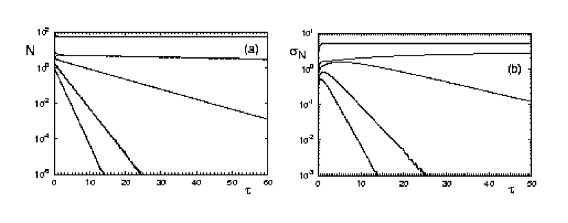
Figure 12: (a) Average number of closed bonds $N$ obtained from stochastic simulations of the master equation for $\gamma=1$ and $N_{t}=1,2,5,10$ and $100$. (b) Variance $\sigma_{N}$ of the cluster size distribution for the same parameters as in (a).

It follows from Eq. (46) that the mean number of closed bonds decay in an exponential way, $N(\tau)=N_{eq}e^{-\bar{p}_{1}(\infty)\tau}$. This is confirmed by Fig. 12a, which shows the corresponding simulation results. For $N_{t}=2,5$ and $10$, we have $\bar{p}_{1}(\infty)=0.5,0.16$ and $9.7\times 10^{-3}$. Numerically we find $0.6,0.13$ and $0.01$, thus the approximation is rather good. In Fig. 12b, we plot numerical results for the standard deviation $\sigma_{N}$. The initial increase of $\sigma_{N}$ is well described by Eq. (44) for the reflecting boundary, thus the boundary has little influence here. Large clusters stay close to the steady state during the time shown and the approximation is applicable. For small clusters, the variance grows larger than the steady state value before is decreases exponentially while the cluster size $N$ approaches zero. The variance contains two time-scales. The second moment of the distribution decreases on the same timescale as the average, while the square of the first moment decreases twice as fast. The long time exponential decrease of $\sigma_{N}$ is thus described by twice the relaxation time as is was found for the average number of bonds.

Although an exact solution for the state probabilities seems to be impossible for the case of an absorbing boundary, more analytical progress can be made if one is only interested in the probability that the cluster dissociates as a whole. For the absorbing boundary, the cluster dissociation rate has been denoted by $D(\tau)$ before. For the reflecting boundary, $D(\tau)$ can be identified as the probability that the state $i=0$ is reached for the first time at time $\tau$ if the system has started in the state $i=N_{t}$ at time $\tau=0$. This is a first passage problem which can be treated with Laplace techniques. Since the transition rates do not depend on absolute time, one can decompose the state probability for $i=0$ into two parts:

$$p_{0}(\tau)=\int_{0}^{\tau}D(\tau^{\prime})p_{0,0}(\tau-\tau^{\prime})d\tau^{\prime}$$ (47)

where $p_{0,0}(\tau)$ is the state probability for state $i=0$ with initial condition $p_{i}(0)=\delta_{i,0}$. $p_{0,0}(\tau)$ can also be interpreted as the probability for having returned to the boundary after time $\tau$. A Laplace transform of the equation leads to an algebraic relation between the Laplace transforms of the three functions:

$$D(s)=\frac{p_{0}(s)}{p_{0,0}(s)}\ .$$ (48)

Here $D(s)=\int_{0}^{\infty}e^{-s\tau}D(\tau)$ denotes the Laplace transform of the function $D(\tau)$. The explicit form of the probability $p_{0}(\tau)$ is given in Eq. (41):

$$p_{0}(\tau)=\left(\frac{1-e^{-(1+\gamma)\tau}}{1+\gamma}\right)^{N_{t}}\ .$$ (49)

The probability $p_{0,0}(\tau)$ can also be calculated with standard techniques Goel and Richter-Dyn (1974):

$$p_{0,0}(\tau)=\left(\frac{1+\gamma e^{-(1+\gamma)\tau}}{1+\gamma}\right)^{N_{t}}\ .$$ (50)

The Laplace transforms of the these two functions are given by

$$p_{0}(s) =\frac{1}{\left(1+\gamma\right)^{N_{t}}}\sum_{i=0}^{N_{t}}\binom{N_{t}}{i}\frac{(-1)^{i}}{s+i(1+\gamma)}$$ (51)

and

$$p_{0,0}(s) =\frac{1}{\left(1+\gamma\right)^{N_{t}}}\sum_{i=0}^{N_{t}}\binom{N_{t}}{i}\frac{\gamma^{i}}{s+i(1+\gamma)}\quad,$$ (52)

so that the Laplace transformed first passage probability time distribution is

$$D(s) =\frac{\sum_{i=0}^{N_{t}}\binom{N_{t}}{i}\frac{(-1)^{i}}{s+i(1+\gamma)}}{\sum_{i=0}^{N_{t}}\binom{N_{t}}{i}\frac{\gamma^{i}}{s+i(1+\gamma)}}\quad.$$ (53)

Unfortunately, the analytical backtransform for $D(s)$ seems to be impossible. However, the mean first passage time can be extracted from this result, because it does not require the backtransfrom Honerkamp (1990):

$$T=\left.\frac{dD(s)}{ds}\right|_{s=0}=\frac{1}{1+\gamma}\left(\sum_{n=1}^{N_{t}}\left\{\binom{N_{t}}{n}\frac{\gamma^{n}}{n}\right\}+H_{N_{t}}\right)\ .$$ (54)

This equation is a polynomial of order $N_{t}-1$ in $\gamma$. The zero order term is the harmonic number $H_{N_{t}}$, so for $\gamma=0$ we recover the result from Eq. (31). In Fig. 13, we plot Eq. (54) as a function of cluster size $N_{t}$ and rebinding rate $\gamma$. As long as $\gamma<1$, cluster lifetime grows only weakly (logarithmically) with cluster size (at least for not too large clusters). For $\gamma>1$, the higher order terms in $\gamma$ take over and the increase in $T$ becomes effectively exponential, as shown in Fig. 13a. In Fig. 13b, it is shown explicitly that increasing $\gamma$ to values larger than unity leads to a strong increase in lifetime. This effect is larger for larger clusters since the number of rebinding events in the dissociation path is larger.

Figure 13: (a) Average lifetime $T$ of adhesion clusters as function of cluster size $N_{t}$ for rebinding rates $\gamma=0.0,0.1,0.5,1,5$ and $10.0$. (b) Average lifetime $T$ as function of rebinding constant $\gamma$ for cluster size $N_{t}=1,2,5,10,20$ and $50$.

V Finite force and finite rebinding

V.1 Deterministic analysis

Force destabilizes the cluster, while rebinding stabilizes it again. It has been shown by Bell that in the framework of the deterministic equation Eq. (4), the cluster remains stable up to a critical force $f_{c}$ Bell (1978). For the following it is helpful to revisit his stability analysis. In equilibrium we have

$$N_{eq}e^{f/N_{eq}}=\gamma(N_{t}-N_{eq})\ .$$ (55)

At small force $f$, this equation has two roots, with the larger one corresponding to a stable equilibrium. As force increases, a saddle-node bifurcation occurs. Above the critical force, no roots exist and the cluster becomes unstable. Exactly at critical loading, the two roots collapse and the slopes of the two terms become equal. This gives an additional equation

$$e^{f_{c}/N_{c}}(1-\frac{f_{c}}{N_{c}})=-\gamma\ .$$ (56)

These two equations allow to determine the critical values for cluster size and force:

$$f_{c}=N_{t}\ \rm plog\left(\frac{\gamma}{e}\right)\quad\text{and}\quad N_{c}=N_{t}\ \frac{\rm plog\left(\frac{\gamma}{e}\right)}{1+\rm plog\left(\frac{\gamma}{e}\right)}\quad,$$ (57)

where the product logarithm $\rm plog(a)$ is defined as the solution $x$ of $xe^{x}=a$. For small forces, the unstable fixed point is very close to zero. This implies that the stable fixed point is an attractor for most initial conditions. Close to the critical force, the unstable fixed point is close to the stable one and only the initial conditions above $N_{c}$ will reach the stable fixed point. Eq. (57) scales in a trivial way with $N_{t}$, but in a complicated way with $\gamma$. For $\gamma<1$, we have $f_{c}\approx\gamma N_{t}/e$. Thus the critical force vanishes with $\gamma$, because the cluster decays by itself with no rebinding. For $\gamma>1$ and up to $\gamma\approx 100$, we have $f_{c}\approx 0.5N_{t}\ln\gamma$. This weak dependence on $\gamma$ shows that the single bond force scale set by $F_{b}$ also determines the force scale on which the cluster as a whole disintegrates. Fig. 14a shows how $f_{c}$ crosses over from linear to logarithmic scaling with $\gamma$.

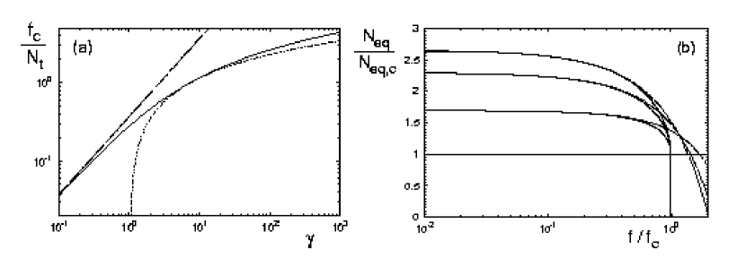
Figure 14: (a) Critical force Eq. (57) in relation to total cluster size, $f_{c}/N_{t}$, as function of the rebinding constant $\gamma$. It scales linearly (dotted curve) at small and logarithmically (dashed curve) for larger $\gamma$. (b) Stable steady value for number of closed bonds normalised by the critical value, $N_{eq}/N_{eq,c}$, for $\gamma=0.1,1$ and $10$ as function of force $f/f_{c}$ for $N_{t}=100$. Numerical results (solid lines) are compared to the approximation Eq. (58) (dashed lines). The horizontal line marks the smallest possible value at the critical force $f_{c}$.

Eq. (55) is an implicit equation which cannot be inverted to give $N_{eq}$ as a function of the model parameters $N_{t}$, $f$ and $\gamma$. In general, $N_{eq}$ decreases from $\gamma N_{t}/(1+\gamma)$ for $f=0$ to $N_{c}$ for $f_{c}$. For small forces we can find an approximate solution by first expanding the exponential function in Eq. (55) to second order in $f/N_{eq}$ and then expanding the resulting quadratic function for $N_{eq}$ to second order in $f/\gamma N_{t}$:

$$N_{eq}\approx\frac{\gamma N_{t}}{1+\gamma}\left[1-\left(\frac{f}{\gamma N_{t}}\right)-\frac{\gamma+1}{2}\left(\frac{f}{\gamma N_{t}}\right)^{2}\right]\quad.$$ (58)

Fig. 14b shows numerical results for $N_{eq}/N_{c}$ in comparison with the low force approximation Eq. (58) for different rebinding constants $\gamma=0.1,1.0$ and $10$ as function of force $f/f_{c}$ and for cluster size $N_{t}=100$.

Figure 15: Deterministic mean lifetime $T$ of a cluster of $N_{t}=100$ bonds for $\gamma=1$ as a function of the force-size ratio $f/N_{t}$. Numerical integration of the deterministic equation (solid line) is compared to the exact solution for vanishing rebinding (dashed line) and the inverse linear scaling (dotted line) predicted close to the critical force.

In the deterministic framework, cluster lifetime is infinite for $f<f_{c}$, because a stationary state exists at $N_{eq}$. For $f>f_{c}$, cluster lifetime is finite, but strongly varies as a function of $N_{t}$, $f$ and $\gamma$. For $f\gg f_{c}$, we can neglect rebinding and use the results from Sec. III, where we found for cluster lifetime

$$T_{det}=E\left(\frac{f}{N_{t}}\right)\approx\frac{e^{-(f/N_{t})}}{1+(f/N_{t})}\ ,$$ (59)

compare Eq. (20). As force $f$ is decreased from above towards the critical value $f_{c}$, rebinding becomes important again and cluster lifetime diverges. To understand this limit, we note that here the system will evolve very slowly, because it is still close to a steady state. Therefore we can expand the time derivative of $N$, compare Eq. (4), for small deviations from the critical state:

$$\frac{dN}{d\tau}\approx\left.\frac{\partial}{\partial f}\left(\frac{dN}{d\tau}\right)\right|_{f_{c},N_{c}}\left(f-f_{c}\right)=-e^{f_{c}/N_{c}}(f-f_{c})=-e^{1+\rm plog(\gamma/e)}(f-f_{c})\ .$$ (60)

In this limit, the lifetime will be dominated by the time spent close to the critical state. The time for a significant change $\Delta N\simeq-1$ in $N$ is

$$T\approx\Delta\tau\approx e^{-(\rm plog(\gamma/e)+1)}\frac{1}{f-f_{c}}\ .$$ (61)

Therefore $T$ diverges like the inverse of $f-f_{c}$. Fig. 15 shows the lifetime of an adhesion cluster derived from numerical integration of the deterministic equation for $\gamma=1$ and $N_{t}=100$ as a function of the force-size ratio $f/N_{t}$. The numerical results are compared to the approximation Eq. (59) for large forces and Eq. (61) for the divergence close to the critical point. Obviously both approximations work well for their respective limits. For different cluster sizes $N_{t}$, the plot remains basically unchanged (not shown), because the forces above $f_{c}$ are already in the range where Eq. (16) predicts scaling with $f/N_{t}$ alone. For different rebinding constants $\gamma$ the results are qualitatively the same, only that the critical force is shifted to different values.

V.2 Stochastic analysis

In general, it seems to be difficult to find a closed-form analytical solution for the state probabilities $p_{i}(\tau)$ for general values of $\gamma$, $f$ and $N_{t}$. In the following, we will derive such an analytical solution for the case $N_{t}=2$ with an absorbing boundary. In principle, solutions can be constructed in the same way for a reflecting boundary or larger clusters, but for increasing cluster size, the analytical procedure quickly becomes intractable. For this reason, we will later use simulations to deal with the general case.

We start by rewriting the master equation Eq. (1) in matrix form:

$$\dot{p}={W}\cdot{p}\ .$$ (62)

For the case $N_{t}=2$ with an absorbing boundary, ${p}=(p_{0},p_{1},p_{2})^{T}$ and

$${W}=\begin{pmatrix}0&r_{1}&0\\ 0&-(r_{1}+g_{1})&r_{2}\\ 0&g_{1}&-r_{2}\end{pmatrix}\ .$$ (63)

Eq. (62) is solved by Honerkamp (1990)

$${p}(\tau)=e^{{W}\tau}\cdot{p}(0)=\sum_{\lambda}c_{\lambda}e^{\lambda\tau}{p}_{\lambda}$$ (64)

where $\lambda$ and ${p}_{\lambda}$ are the eigenvalues and eigenvectors of ${W}$, respectively. The coefficients $c_{\lambda}$ have to be determined from the initial condition

$${p}(0)=\sum_{\lambda}c_{\lambda}{p}_{\lambda}\ .$$ (65)

Since the absorbing state ${p}_{0}=(1,0,0)^{T}$ is a stationary state, the corresponding eigenvalue $\lambda_{0}=0$. The other two eigenvalues are negative and correspond to transient states:

$$\lambda_{1,2}=-(\Omega\pm\omega)$$ (66)

with $\Omega$ and $\omega$ being defined as

$$\Omega=(r_{1}+r_{2}+g_{1})/2\quad\text{and}\quad\omega=\sqrt{\Omega^{2}-r_{1}r_{2}}\ .$$ (67)

Note that $0<\omega<\Omega$ and hence $\lambda_{1,2}<0$. The transient eigenstates are

$${p}_{1}=\frac{1}{g_{1}}\begin{pmatrix}\lambda_{2}+r_{1}\\ \lambda_{1}+r_{2}\\ g_{1}\end{pmatrix}\quad\text{and}\quad{p}_{2}=\frac{1}{g_{1}}\begin{pmatrix}\lambda_{1}+r_{1}\\ \lambda_{2}+r_{2}\\ g_{1}\end{pmatrix}\ .$$ (68)

The three eigenstates ${p}_{\lambda}$ are linearly independent and form a basis of the state space of the cluster. With the initial condition $p_{i}=\delta_{i,N_{t}}$, that is ${p}(0)=(0,0,1)^{T}$, the coefficients $c_{\lambda}$ follow from Eq. (65) as

$$c_{\lambda_{0}}=1\ ,\quad c_{\lambda_{1}}=\frac{\lambda_{2}+r_{2}}{\lambda_{2}-\lambda_{1}}\quad\text{and}\quad c_{\lambda_{2}}=-\frac{\lambda_{1}+r_{2}}{\lambda_{2}-\lambda_{1}}\ .$$ (69)

The final result then can be written as

$$p_{0}(\tau) = 1-\left[\cosh(\omega\tau)+\frac{\Omega}{\omega}\sinh(\omega\tau)\right]e^{-\Omega\tau}\ ,$$

$$p_{1}(\tau) = \frac{r_{2}}{\omega}\sinh(\omega\tau)e^{-\Omega\tau}\ ,$$ (70)

$$p_{2}(\tau) = \left[\cosh(\omega\tau)+\frac{\Omega-r_{2}}{\omega}\sinh(\omega\tau)\right]e^{-\Omega\tau}\ .$$

There is a competition between the hyperbolic terms, which grow on the time-scale $1/\omega$, and the exponential terms, which decrease on the time-scale $1/\Omega$. Since $\omega<\Omega$, the exponential terms will win and only the stationary state survives.

With the exact solution Eq. (70), one now can calculate any quantity of interest. For example, the mean number of bonds, $N(\tau)=\sum_{i}ip_{i}$, follows as

$$N(\tau)=\left[2\cosh(\omega\tau)+\frac{r_{1}+g_{1}}{\omega}\sinh(\omega\tau)\right]e^{-\Omega\tau}\ .$$ (71)

The dissocation rate for the cluster as a whole as given by $D(\tau)=r_{1}p_{1}=\dot{p}_{0}$, resulting in

$$D(\tau)=\frac{r_{1}r_{2}}{\omega}\sinh(\omega\tau)e^{-\Omega\tau}\ .$$ (72)

One easily checks that normalization is correct, $\int_{0}^{\infty}D(\tau)d\tau=1$. Mean cluster lifetime $T$ now follows as

$$T=\int_{0}^{\infty}\tau D(\tau)d\tau=\frac{1}{2}\left(2e^{-f}+e^{-f/2}+\gamma e^{-3f/2}\right)\ .$$ (73)

As shown in the preceding sections for special cases, force leads to exponentially decreased lifetimes, while rebinding leads to polynomial terms in $\gamma$ up to order $N_{t}-1$.

Figure 16: State probabilities $p_{i}$ as a function of time $\tau$ for $N_{t}=10$ with $\gamma=1$ for force $f=0.1,1,3$ and $10$ (a - d). In (a), the numerical solution is compared with the leakage approximation (dotted lines). The intermediate force values are chosen below and above the critical force $f_{c}=0.278N_{t}$.

Although the eigenvalue analysis can be used also for the general case of arbitrary cluster size, in this case it is more efficient to use exact stochastic simulations as described in Sec. II.2. In Fig. 16 numerical solutions of the state occupancy probabilities $\{p_{i}\}_{i=0}^{N_{t}}$ are plotted for $N_{t}=10$ with $\gamma=1$ for four different forces $f=0.1,1,3$ and $50$. This figure corresponds to Fig. 2 for vanishing rebinding and Fig. 11 for vanishing force. For small force, the numerical solutions compare well with the approximation Eq. (46) introduced for vanishing force. For larger force, but still below the critical force, the state probabilities still decrease exponentially for large times, but the approximation Eq. (46) breaks down, because the reference distribution $\{\bar{p}_{i}(\infty)\}_{i=0}^{N_{t}}$ now had to be replaced by the unknown steady state for the case of finite force. If force is increased beyond the critical force ($f_{c}=2.78$ for $\gamma=1$), a simple description is not available, because equilibration and decay occur on the same timescale. For very large force, the behavior of the adhesion cluster approaches that for vanishing rebinding, with the analytical solution Eq. (23).

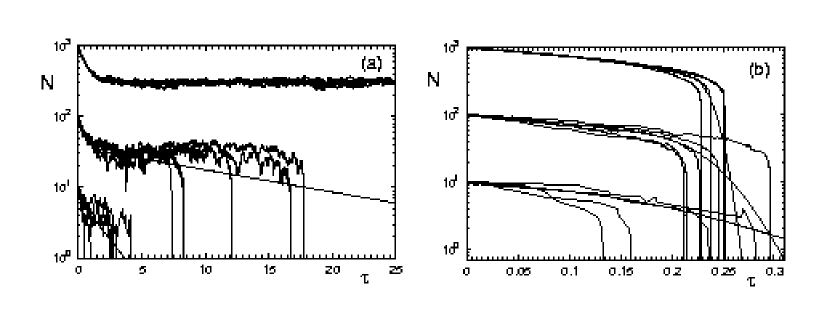
Figure 17: Single simulation trajectories for $N_{t}=10,100$ and $100$ for $\gamma=1$ and at two different forces (a) $f=0.25N_{t}<f_{c}$ and (b) $f=N_{t}>f_{c}$. Representative trajectories are compared to the average number $N$ of closed bonds resulting from averaging over a large number of such trajectories.

Fig. 17 demonstrates that the decay process changes dramatically as force is increased above the critical value. It displays trajectories of individual clusters with initially $N_{t}=N_{0}=10,100$ and $1000$ closed bonds in comparison with the average number of bonds derived from a large number of these trajectories. Since $f_{c}=0.278N_{t}$ for $\gamma=1$, Fig. 17a with $f=0.25N_{t}$ is below the critical value. For the largest cluster, the system equilibrates towards the steady state and then fluctuate around this value with very rare encounters of the absorbing boundary. For the smaller clusters, however, fluctuations towards the absorbing boundary frequently lead to loss of individiual realizations. As a result, the average number of closed bonds decays exponentially on a much faster timescale. Fig. 17a with $f=N_{t}$ is above the critical force and the behavior is changed qualitatively. A steady state does not exist anymore and the clusters do not decay by fluctuations, but the size of each adhesion cluster is continuously reduced. Clusters of different size now decay on the same timescale and rebinding events are very rare in comparison to rupture events.

Figure 18: Average number of closed bonds $N$ for $N_{t}=1,10,100$ and $1000$, $\gamma=1$ and (a) $f/N_{t}=0.25$ and (b) $f/N_{t}=1$. In (a), the numerical results are compared to exponentially decaying curves $\sim e^{-a\tau}$ (dashed lines) with $a=1.28,0.52,0.072$ and $0.0009$ for increasing bond number.

Fig. 18 plots numerical results for the average number of closed bonds $N$ as function of time $\tau$ for two different values of $f/N_{t}$ and for cluster sizes $N_{t}=1,10,10^{2}$ and $10^{3}$. For $f=0.25N_{t}<f_{c}$, after initial relaxation all curves decay exponentially. For $f=N_{t}>f_{c}$, the larger clusters show a steep decrease in average cluster size at the end of the decay due to the effects of shared loading. For the small clusters, the average cluster size decreases slowly since cooperative effects are small.

Figure 19: Variance $\sigma_{N}$ for forces (a) $f=0.25N_{t}$ and (b) $f=N_{t}$ for $\gamma=1$ and $N_{t}=1,10,100$ and $1000$.

Fig. 19 plots the variance $\sigma_{N}(\tau)$ of the distribution $p_{i}$ for the two force values used in the two previous figures. Below the critical force the behavior is similar to that for vanishing force depicted in Fig. 12. The variance decreases exponentially after having traversed a maximum. For forces above the critical force, a different behavior arises. After growing as expected in the initial phase, the variance displays a sharp peak. This effects becomes more pronounced the larger cluster size.

Figure 20: Comparison of stochsatic and deterministic results for the average number of closed bonds $N$ derived from numerical solutions of the master equation (solid lines) and from integration of the deterministic equation (dashed curves) for cluster sizes $N_{t}=10,100$ and $1000$ and forces (a) $f/N_{t}=0.1$ and (b) $1.0$. The rebinding rate is $\gamma=1$.

In Fig. 20 a comparison of the average number of closed bonds in the stochastic and the determinsitic description is shown. $N(\tau)$ is plotted for cluster sizes $N_{t}=10,100$ and $1000$ for the forces $f/N_{t}=0.1$ and $1.0$ and the rebinding rate $\gamma=1.0$. For small forces $f<f_{c}$, the average number of closed bonds equilibrates towards the steady state and remains constant thereafter. The fluctuations occuring in the stochastic description lead to a slow decrease of $N$. Above the critical force, the deterministic clusters decay as well, and in a more abrupt way than the stochastic average.

Figure 21: Dissociation rate $D$ of the overall cluster for $\gamma=1$ and $N_{t}=1,5,10,25,100$ and $1000$. (a) $f=0.25N_{t}$ and (b) $f=N_{t}$.

We now turn to the dissociation rate of the overall cluster as a function of the model parameters. For $\gamma=1$ and $f=0.25N_{t}$ and $N_{t}$, that is below and above the critical force, numerical results are plotted in Fig. 21. For a single bond, dissociation is a Poisson process with the maximum at $\tau=0$ and an exponentially decreasing dissociation rate $D=r(1)p_{1}=e^{f}e^{-e^{f}\tau}$. For larger clusters and below the critical force, fluctuations to the absorbing boundary determine the rate of dissociation, which vanishes at $\tau=0$, goes through a maximum and then decreases exponentially with time. As explained above, the exponential decay follows because decay proceeds by rare fluctuations from the steady state towards the absorbing boundary. Above the critical force, the dissociation rate for $N_{t}>1$ becomes more sharply peaked and cannot be described with single exponential curves. A steady state does not exist anymore and dissociation does not proceed by fluctuations. The trajectories in Fig. 17 have shown that adhesion clusters decay fairly abrupt towards the end of the decay as a consequence of shared loading. This cooperative instability is the reason for the sharp dissociation distribution for large clusters under super-critical loading. The single bond that lacks these cooperativity, still shows the exponential dissociation rate which is now the slowest decaying for the given force size ratio.

Whereas results for the dissociation rate have to be obtained numerically, the average lifetime can be calculated analytically van Kampen (1992). The basic idea here is to sum the average times for any possible pathway leading from the initial cluster size $N_{0}$ towards dissociation at the absorbing boundary $i=0$ with its appropriate statistical weight. One can show that the lifetime $T_{N_{t},N_{0}}$ of a cluster with a total of $N_{t}$ molecular bonds of which $N_{0}$ are closed initially satisfies the equation van Kampen (1992)

$$g(N_{0})\left(T_{N_{t},N_{0}+1}-T_{N_{t},N_{0}}\right)+r(N_{0})\left(T_{N_{t},N_{0}-1}-T_{N_{t},N_{0}}\right)=-1\ .$$ (74)

The left hand side can be considered to be the adjoint operator of the master equation acting on the average lifetime $T_{N_{t},N_{0}}$. For the initial condition $N_{0}=N_{t}$, the equation is solved exactly by

$$T=T_{N_{t},N_{t}}=\sum_{i=1}^{N_{t}}\frac{1}{r(i)}+\sum_{i=1}^{N_{t}-1}\sum_{j=i+1}^{N_{t}}\frac{\prod_{k=j-i}^{j-1}g(k)}{\prod_{k=j-i}^{j}r(k)}\ ,$$ (75)

where the first term is the result Eq. (30) for vanishing rebinding and the second term results in a polynomial of order $N_{t}-1$ in $\gamma$. For $f=0$, Eq. (75) is identical to the earlier result Eq. (54) obtained by Laplace transforms. Both expressions are polynomials of order $N_{t}-1$ in $\gamma$, but in the general case from Eq. (75), the coefficients depend on force. For $N_{t}=2$, we obtain the result from Eq. (73). For $N_{t}=3$, we find

$$T=e^{-f}+\frac{e^{-f/2}}{2}+\frac{e^{-f/3}}{3}+\gamma\left(\frac{e^{-5f/6}}{6}+e^{-3f/2}\right)+\gamma^{2}\frac{e^{-11f/6}}{3}\ .$$ (76)

For $N_{t}=2$ and $3$, $T$ can also be derived by explicitly summing over all possible dissociation paths. For larger $N_{t}$, direct summation becomes intractable and the results following from the general formula Eq. (75) become rather lengthy. In general, force always affects most strongly those terms of highest order in $\gamma$, thus for $\gamma>1$, application of force is therefore an efficient way to reduce average lifetime $T$. For $\gamma<1$, $T$ is dominated by those terms of lowest order in $\gamma$, thus here the reduction of lifetime with increasing force is not modulated by rebinding.

Figure 22: Average lifetime $T$ according to Eq. (75) (solid lines) of adhesion clusters with $N_{t}=1,2,5,10,15$ and $25$ as a function of $f/N_{t}$ for (a) $\gamma=0.1$ and (b) $\gamma=1$. The critical forces for these rebinding rates are $f_{c}/N_{t}=0.0355$ and $0.278$, respectively, where the deterministic results for the lifetimes (dashed lines) diverge.

Fig. 22 shows the average lifetime of adhesion clusters of size $N_{0}=1,2,5,10,15$ and $25$ as a function of force-size ratio $f/N_{t}$ for the rebinding constants $\gamma=0.1$ and $\gamma=1.0$. For small forces, $f<1$, the average lifetime plateaus at the value given by Eq. (54). For large forces, $f>N_{t}$, that is, when the force on each single bond is larger than the intrinsic force scale, the limit of vanishing rebinding applies (for $N_{t}=1$ lifetime is independent of $\gamma$, compare also Fig. 15). The critical forces for the given rebinding rates are $f_{c}=0.0355N_{t}$ and $f_{c}=0.278N_{t}$. In the intermediate force range, roughly around $f_{c}$, the lifetime is reduced from the zero force to the zero rebinding limit. This reduction is dramatic for large clusters ($N_{t}\geq 10$) with appreciable rebinding ($\gamma\geq 1$), where the lifetime is reduced by orders of magnitude. We also show the lifetime following from the deterministic framework, which provides a lower limit for the lifetime at large forces, because here the largest clusters have the shortest lifetimes for a given force size ratio $f/N_{t}$. Below the critical force the deterministic lifetime is infinite and the stochastic curves approach the plateaus Eq. (54) determined by fluctuations towards the absorbing boundary.

Figure 23: Average cluster lifetime $T$ (a) as function of rebinding rate $\gamma$ for $N_{t}=10$ and $f/N_{t}=0,0.1,0.3,0.6$ and $1$ and (b) as function of cluster size $N_{t}$ for $\gamma=1.0$ and $f=0,1,2$ and $10$.

Fig. 23a demonstrates the influence of rebinding on the average lifetime at different levels of force. Here we show average lifetime $T$ as function of $\gamma$ for $N_{t}=10$ and for increasing values of force. For $f=0$ the curves are as depicted in Fig. 13. Increasing force reduces the lifetime strongly and leads to an almost constant lifetime for different $\gamma$ (compared the strong increase for $f=0$). Only when rebinding is sufficiently strong that force is smaller than the critical force, $f<f_{c}$, lifetime begins to grow. The increase observed then is similar to that for vanishing force, only that the absolute value of lifetime is smaller. For example, for $f=0.6N_{t}$, the cluster grows strongly for $g\geq 5$ where the critical force is $f_{c}=0.82N_{t}$; for $f=N_{t}$ the strong increase is observed for $g\geq 10$, for which the critical force is $f_{c}=1.15N_{t}$. A similar effect is observed for the dependence of average lifetime on cluster size, see Fig. 23b. At small $N_{t}$, cluster lifetime grows strongly at large forces according to Eq. (30) due to shared loading. For larger $N_{t}$, lifetime grows slowly until $N_{t}$ is large enough that $f_{c}\geq f$ is reached. Above this size, $T$ grows on a rate comparable to that for vanishing or small force. For $\gamma=0.1$, the increase of $T$ with $N_{t}$ is slow throughout the shown range of $N_{t}$.

VI Discussion

In this paper, we have presented a detailed analysis of the stochastic dynamics of an adhesion cluster of size $N_{t}$ under shared loading $f$ and with rebinding rate $\gamma$. The corresponding master equation has been solved exactly for several special cases. For vanishing rebinding ($\gamma=0$), the exact solution Eq. (24) could be constructed because cluster decay is a sequence of Poisson processes. For vanishing force ($f=0$), we deal with a linear problem, which can be treated with standard techniques. In the case of natural boundaries (that is for a reflecting boundary at $i=0$), the exact solution Eq. (41) follows with the help of a generating function. In the general case of finite force $f$ and finite rebinding rate $\gamma$, for the case $N_{t}=2$ and an absorbing boundary we used an eigenvalue analysis to derived the exact solution Eq. (70). In principle, the same method can also be applied for a reflecting boundary or for larger clusters, but this does not lead to simple analytical results.

For vanishing force ($f=0$) and an absorbing boundary at $i=0$, we introduced the ‘leakage approximation’ (also known as ’local thermal equilibrium description’ in the theory of protein folding), which treats the absorbing boundary as a small perturbation to the exactly solved case of the reflecting boundary. The resulting formulae given in Eq. (46) work well if average cluster lifetime $T$ is much larger than the internal time scale $1/(1+\gamma)$ (that is for large clusters or strong rebinding). All other cases have been treated with exact stochastic simulations using the Gillespie algorithm, which for large clusters is more efficient than the eigenvalue analysis. Moreover, the study of single simulation trajectories offers valuable insight into the typical nature of unbinding trajectories expected for experiments.

Once the master equation is solved, either exactly or numerically, all quantities of interest can be calculated. In this paper, we focused on the mean number of closed bonds as a function of time, $N(\tau)$, and the dissociation rate for the overall cluster, $D(\tau)$. The first moment of $D(\tau)$ then gives the mean cluster lifetime $T$. In this paper, we derived an exact solution $T=T(N_{t},f,\gamma)$ from the adjoint master equation, see Eq. (75). For the special cases of vanishing rebinding and vanishing force, we also showed how the exact formulae for $T$ can be derived via completely different routes. The result for $T=T(N_{t},f)$ from Eq. (30) follows from the unique dissociation path without rebinding, while the result for $T=T(N_{t},\gamma)$ from Eq. (54) can be derived with Laplace techniques as a mean first passage time for the case of a reflecting boundary. In order to assess the role of fluctuations, we also calculated the standard deviations $\sigma_{N}$ and $\sigma_{T}$ for the distributions of the number of closed bonds and cluster lifetimes, respectively.

A special focus of this paper was a detailed comparision between the stochastic and determinstic treatment. Regarding mean cluster lifetime, the deterministic treatment is rather good in the case of vanishing rebinding, although it underestimates the plateau value for cluster lifetime at small force. In the presence of rebinding, the deterministic treatment fails, because it includes neither the effect of fluctuations nor the effect of an absorbing boundary. In particular, the deterministic treatment does not predict finite lifetime below the critical force $f_{c}$, when clusters decay due to fluctuations towards the absorbing boundary. Only at very large force, when rebinding becomes irrelevant, does the deterministic treatment work well again. Regarding the average number of closed bonds, the deterministic model fails because it does not correctly treat the non-linearity in the rupture rate. This effect is most evident for small clusters and at late stage of rupture. In general, the mean number of closed bonds in the stochastic model decay in a smoother way than in the deterministic model, which typically shows an abrupt decay in late stage. This abrupt decay in fact is typical for shared loading and shows up in the stochastic model when one studies single simulation trajectories. In this sense, the deterministic model makes an interesting prediction which should be confirmed in experiment, albeit not on the level of the first moment, as suggested by the deterministic model, but rather on the level of single trajectories, as suggested by the stochastic model.

Our results can now be used to evaluate a large range of different experimental situations. The stochastic dynamics of adhesion clusters under force can be quantitatively studied with many different techniques, including atomic force microscopy, optical tweezers, magnetic tweezers, the biomembrane force probe, flow chambers, and the surface force apparatus. In all of these cases, by measuring cluster lifetime $T$ and two out of the three parameters $N_{t}$, $f$ and $\gamma$, the third parameter can be estimated with the help of our exact results. In general, our exact results nicely show how mean cluster lifetime $T$ varies with cluster size $N_{t}$, force $f$ and rebinding rate $\gamma$. For example, if the single bond lifetime was one second ($k_{0}=1/s$), for $f=0$ and $\gamma=0$ a cluster lifetime $T$ of one minute could only be achieved with $10^{26}$ bonds, because in this case, cluster lifetime scales only logarithmically with cluster size. However, for a rebinding rate $\gamma=1$ ($k_{on}=k_{0}$), only $N_{t}=10$ bonds are necessary, because lifetime scales strongly with rebinding, $T\sim\gamma^{N_{t}-1}$. Increasing force to $f=10$ would decrease lifetime to $T=0.05$ s, because $T$ is exponentially decreased by $f$. To reach one minute again, cluster size or rebinding rate had to be increased such that $f<f_{c}$. This implies $N_{t}>50$ or $\gamma>10$. It is important to note that these predictions are based on the assumption of rigid force transducers. In many experimental situations of interest, the force transducer will be subject to elastic deformations or even to viscous relaxation processes, like for example when pulling on cells Benoit et al. (2000). In order to focus on generic aspects of adhesion clusters, here we only studied the minimal model for stochastic dynamics under force.

Our results can also be applied to experiments in cell adhesion. For example, the biomembrane force probe with linear loading has recently been used to study the decay of $\alpha_{\nu}\beta_{3}$-integrin clusters induced on the surface of endothelial cells Prechtel et al. (2002); Erdmann and Schwarz (2004b). If one makes sure that the clusters do not actively grow during the time of dissociation, similar experiments could now be done also for constant loading. Because in these kinds of experiments the exact cluster size is usually unknown, one had to convolute our results with a Poisson distribution for an estimated average number of bonds Chesla et al. (1998); Zhu (2000). Recently, our result for the average cluster lifetime of two bonds under shared force and with rebinding, Eq. (73), has been applied to the analysis of flow chamber data on leukocyte tethering through L-selectin Schwarz and Alon (2004). Since in this case force can be calculated as a function of shear flow, our formula can be used to the estimate rebinding rate, which in this case turns out to be surprisingly large. This in turn explains why dissociation dynamics in L-selectin mediated leukocyte tethering appears to be first order: for large rebinding, the leakage approximation is rather good, and decay is exponential.

Our results can not be directly applied to adhesion clusters which compensate for force-induced decay by active growth, as it has been found experimentally for focal adhesions Riveline et al. (2001). Yet there are also interesting lessons for focal adhesions which can be learned from our model. For example, our stochastic analysis confirms the prediction from the deterministic stability analysis that cluster stability changes strongly around the critial value $f_{c}$ (although small clusters tend to decay also at smaller force due to fluctuations towards the absorbing boundary). It is interesting to note that recent experiments measuring internally generated force at single focal adhesions suggest that $f/N_{t}$, the most important scaling variable of our analysis, is roughly constant for different cell types Balaban et al. (2001); Tan et al. (2003). It is therefore tempting to speculate that focal adhesions (or subsets of focal adhesions) are regulated to be loaded close to the critical value $f_{c}/N_{t}=\rm plog(\gamma/e)$ from Eq. (57). In this way, cells could quickly increase force on single bonds by small changes in actomyosin contractility. Large force on single closed bonds in turn might trigger certain signaling events in focal adhesions, possibly by mechanically opening up certain signaling domains Isralewitz et al. (2001). Our speculation provides a simple way to estimate the rebinding rate, which is very hard to measure experimentally. Using compliant substrates, it has been found that focal adhesions are characterized by a stress constant $\sim 5.5$ nN/$\mu m^{2}$ Balaban et al. (2001); Tan et al. (2003). We do not know which of the many different proteins in focal adhesions defines the weak link which most likely ruptures under force, but we expect that it will have a similar area density as the integrin receptors, which are expected to have a typical distance between 10 and 30 nm, corresponding to $10^{4}$ and $10^{3}$ molecules per $\mu m^{2}$, respectively. To obtain a lower estimate for $\gamma$, we therefore use $F_{c}=5.5$ nN and $N_{t}=10^{4}$. For activated $\alpha_{5}\beta_{1}$-integrin binding to fibronectin, recent single molecule experiments obtained for the molecular parameter values $k_{0}=0.012$ Hz and $F_{b}=9$ pN Li et al. (2003). Therefore the rebinding rate can be estimated to be at least $\gamma=0.2$, that is $k_{on}=0.002$ Hz in dimensional units. Based on future experimental input, it would be interesting to extend our model of passive decay to active processes resulting in cluster growth under force.

Finally we want to comment that our model might also be applied to situations in materials science which are not directly related to biomolecular receptor-ligand pairs. One example is sliding friction, which recently has been modeled as dynamic formation and rupture of bonds under force Filippov et al. (2004). In general, we expect that many more cohesion phenomena in materials can be successfully modeled as dynamic interplay between rupture and rebinding.

Acknowledgments: This work was supported by the German Science Foundation through the Emmy Noether Program.

References

- Alberts et al. (2002) B. Alberts, A. Johnson, J. Lewis, M. Raff, K. Roberts, and P. Walter, Molecular biology of the cell (Garland Science, New York, 2002), 4th ed.
- Evans (2001) E. Evans, Annu. Rev. Biophys. Biomol. Struct. 30, 105 (2001).
- Merkel (2001) R. Merkel, Phys. Rep. 346, 344 (2001).
- Weisel et al. (2003) J. W. Weisel, H. Shuman, and R. I. Litvinov, Curr. Opin. Struct. Biol. 13, 227 (2003).
- Florin et al. (1994) E.-L. Florin, V. T. Moy, and H. E. Gaub, Science 264, 415 (1994).
- Evans and Ritchie (1997) E. Evans and K. Ritchie, Biophys. J. 72, 1541 (1997).
- Rief et al. (1997) M. Rief, M. Gautel, F. Oesterhelt, J. M. Fernandez, and H. E. Gaub, Science 276, 1109 (1997).
- Kellermayer et al. (1997) M. S. Z. Kellermayer, S. B. Smith, H. L. Granzier, and C. Bustamante, Science 276, 1112 (1997).
- Merkel et al. (1999) R. Merkel, P. Nassoy, A. Leung, K. Ritchie, and E. Evans, Nature 397, 50 (1999).
- Simson et al. (1999) D. A. Simson, M. Strigl, M. Hohenadl, and R. Merkel, Phys. Rev. Lett. 83, 652 (1999).
- Alon et al. (1995) R. Alon, D. A. Hammer, and T. A. Springer, Nature 374, 539 (1995).
- Pierres et al. (2002) A. Pierres, D. Touchard, A.-M. Benoliel, and P. Bongrand, Biophys. J. 82, 3214 (2002).
- Lauffenburger and Linderman (1993) D. A. Lauffenburger and J. J. Linderman, Receptors: models for binding, trafficking, and signalling (Oxford University Press, Oxford, 1993).
- Izrailev et al. (1997) S. Izrailev, S. Stepaniants, M. Balsera, Y. Oono, and K. Schulten, Biophys. J. 72, 1568 (1997).
- Shillcock and Seifert (1998) J. Shillcock and U. Seifert, Phys. Rev. E 57, 7301 (1998).
- Heymann and Grubmüller (2000) B. Heymann and H. Grubmüller, Phys. Rev. Lett. 84, 6126 (2000).
- Braun et al. (2004) O. Braun, A. Hanke, and U. Seifert (2004), cond-mat/0402496.
- Zhang et al. (2002) X. Zhang, E. Wojcikiewicz, and V. T. Moy, Biophys. J. 83, 2270 (2002).
- Li et al. (2003) F. Li, S. D. Redick, H. P. Erickson, and V. T. Moy, Biophys. J. 84, 1252 (2003).
- Baumgartner et al. (2000) W. Baumgartner, P. Hinterdorfer, W. Ness, A. Raab, D. Vestweber, H. Schindler, and D. Drenckhahn, Proc. Nat. Acad. Sci. USA 97, 4005 (2000).
- Fritz et al. (1998) J. Fritz, A. G. Katopodis, F. Kolbinger, and D. Anselmetti, Proc. Nat. Acad. Sci. USA 95, 12283 (1998).
- Evans et al. (2001) E. Evans, A. Leung, D. Hammer, and S. Simon, Proc. Natl. Acad. Sci. USA 98, 3784 (2001).
- Bell (1978) G. I. Bell, Science 200, 618 (1978).
- Dembo et al. (1988) M. Dembo, D. C. Torney, K. Saxman, and D. Hammer, Proc. R. Soc. Lond. B 234, 55 (1988).
- Hammer and Apte (1992) D. A. Hammer and S. M. Apte, Biophys. J. 63, 35 (1992).
- Chang et al. (2000) K.-C. Chang, D. F. J. Tees, and D. A. Hammer, Proc. Natl. Acad. Sci. USA 97, 11262 (2000).
- Seifert (2000) U. Seifert, Phys. Rev. Lett. 84, 2750 (2000).
- Seifert (2002) U. Seifert, Europhys. Lett. 58, 792 (2002).
- Prechtel et al. (2002) K. Prechtel, A. R. Bausch, V. Marchi-Artzner, M. Kantlehner, H. Kessler, and R. Merkel, Phys. Rev. Lett. 89, 028101 (2002).
- Zuckermann and Bruinsma (1995) D. Zuckermann and R. Bruinsma, Phys. Rev. Lett. 74, 3900 (1995).
- Lipowsky (1996) R. Lipowsky, Phys. Rev. Lett. 77, 1652 (1996).
- Weikl and Lipowsky (2001) T. R. Weikl and R. Lipowsky, Phys. Rev. E 64, 011903 (2001).
- Albersdörfer et al. (1997) A. Albersdörfer, T. Feder, and E. Sackmann, Biophys. J. 73, 245 (1997).
- Chesla et al. (1998) S. E. Chesla, P. Selvaraj, and C. Zhu, Biophys. J 75, 1553 (1998).
- Bruinsma et al. (2000) R. Bruinsma, A. Behrisch, and E. Sackmann, Phys. Rev. E 61, 4253 (2000).
- Hammer and Lauffenburger (1987) D. A. Hammer and D. A. Lauffenburger, Biophys. J. 52, 475 (1987).
- Cozens-Roberts et al. (1990) C. Cozens-Roberts, D. A. Lauffenburger, and J. A. Quinn, Biophys. J. 58, 841 (1990).
- Tees et al. (2001) D. F. J. Tees, J. T. Woodward, and D. A. Hammer, J. Chem. Phys. 114, 7483 (2001).
- Zhu (2000) C. Zhu, J. Biomech. 33, 23 (2000).
- Erdmann and Schwarz (2004a) T. Erdmann and U. S. Schwarz, Phys. Rev. Lett. 92, 108102 (2004a).
- Erdmann and Schwarz (2004b) T. Erdmann and U. S. Schwarz, Europhys. Lett. 66, 603 (2004b).
- Schwarz and Alon (2004) U. S. Schwarz and R. Alon, Proc. Natl. Acad. Sci. USA 101, 6940 (2004).
- Balaban et al. (2001) N. Q. Balaban, U. S. Schwarz, D. Riveline, P. Goichberg, G. Tzur, I. Sabanay, D. Mahalu, S. Safran, A. Bershadsky, L. Addadi, et al., Nat. Cell Biol. 3, 466 (2001).
- Schwarz et al. (2002) U. S. Schwarz, N. Q. Balaban, D. Riveline, A. Bershadsky, B. Geiger, and S. A. Safran, Biophys. J. 83, 1380 (2002).
- Tan et al. (2003) J. L. Tan, J. Tien, D. M. Pirone, D. S. Gray, K. Bhadriraju, and C. S. Chen, Proc. Natl. Acad. Sci. USA 100, 1484 (2003).
- Alon et al. (1997) R. Alon, S. Chen, K. D. Puri, E. B. Finger, and T. A. Springer, J. Cell Biol. 138, 1169 (1997).
- Orsello et al. (2001) C. E. Orsello, D. A. Lauffenburger, and D. A. Hammer, Trends Biotech. 19, 310 (2001).
- Jeppesen et al. (2001) C. Jeppesen, J. Y. Wong, T. L. Kuhl, J. N. Israelachvili, N. Mullah, S. Zalipsky, and C. M. Marques, Science 293, 465 (2001).
- Moreira et al. (2003) A. G. Moreira, C. Jeppesen, F. Tanaka, and C. M. Marques, Europhys. Lett. 62, 876 (2003).
- Moreira and Marques (2004) A. G. Moreira and C. M. Marques, J. Chem. Phys. 120, 6229 (2004).
- van Kampen (1992) N. G. van Kampen, Stochastic processes in physics and chemistry (Elsevier, Amsterdam, 1992).
- Honerkamp (1990) J. Honerkamp, Stochastische dynamische Systeme (VCH, Weinheim, 1990).
- Gillespie (1976) D. T. Gillespie, J. Comput. Phys. 22, 403 (1976).
- Gillespie (1977) D. T. Gillespie, J. Phys. Chem. 81, 2340 (1977).
- Goldstein and Wofsy (1996) B. Goldstein and C. Wofsy, Immunology Today 17, 77 (1996).
- McQuarrie (1963) D. A. McQuarrie, J. Chem. Phys. 38, 433 (1963).
- Zwanzig (1995) R. Zwanzig, Proc. Natl. Acad. Sci. 94 (1995).
- Goel and Richter-Dyn (1974) N. S. Goel and N. Richter-Dyn, Stochastic models in biology (Academic Press, New York, 1974).
- Benoit et al. (2000) M. Benoit, D. Gabriel, G. Gerisch, and H. E. Gaub, Nat. Cell Biol. 2, 313 (2000).
- Riveline et al. (2001) D. Riveline, E. Zamir, N. Q. Balaban, U. S. Schwarz, B. Geiger, Z. Kam, and A. D. Bershadsky, J. Cell Biol. 153, 1175 (2001).
- Isralewitz et al. (2001) B. Isralewitz, M. Gao, and K. Schulten, Curr. Opin. Struct. Biol. 11, 224 (2001).
- Filippov et al. (2004) A. E. Filippov, J. Klafter, and M. Urbakh, Phys. Rev. Lett. 92, 135503 (2004).