Phonon structure in point-contact spectra of MgB₂

Abstract

In strong-coupling superconductors with a short electron mean free path the self-energy effects in the superconducting order parameter play a major role in the phonon manifestation of the point-contact spectra at above-gap energies. We compare the expressions for the nonlinear conductivity of tunnel, ballistic, and diffusive point-contacts and show that these expression are similar and correspond to the measurements of the phonon structure in the point-contact spectra for the $\pi$-band  of MgB₂.

I Introduction

The inelastic point-contact spectra of phonons in metals are based on expansion of the nonlinear $I-V$ characteristic in terms proportional to $\ d/l_{\varepsilon}$, where $d$ is the characteristic size of metallic nanoconstriction connecting two bulk metal half-spaces and $l_{\varepsilon}$ is the inelastic electron mean free path KOS ; Yan2000 .

If $d$ is smaller than the electron mean free path $l$  ($l^{-1}=l_{i}^{-1}+l_{\varepsilon}^{-1}$, $l_{i}$ is the elastic mean free path), the electrons flow through the contact ballistically. In opposite cases $(d\gg l)$ they perform a diffusive motion, but if the energy relaxation length $\Lambda_{\varepsilon}\approx\sqrt{l_{i}l\varepsilon}$ remains larger than $d$, their movement inside the constriction is conservative, and the inelastic point-contact spectroscopy is still possible KulYan ; KSS .

In the superconducting state a new characteristic length appears: the size of the Cooper pair or the coherence length $\xi,$ and the additional nonlinear  features emerge being proportional to the expansion of the so called ”excess” current in terms proportional to $d/\xi.$ In all the cases considered, the size of the contact is smaller than the corresponding characteristic length scale: $\xi,\,l_{\varepsilon},\Lambda_{\varepsilon}$ etc.

The zero-approximation in expansion of $I(V)$ in $d/l_{\varepsilon}$ is the ohmic current considered by Sharvin Sha . From the Sharvin’s formula the characteristic size $d$ of the contact can be determined in the ballistic limit. The second derivative of the first approximation in expansion of $I(V)$ in $d/l_{\varepsilon}$ is directly proportional to the spectral function of electron-phonon interaction (PC EPI) $\ g_{PC}(\omega)=\alpha_{PC}^{2}\left(\omega\right)F\left(\omega\right)$ of the specific point-contact transport both in the normal and in the superconducting states KOS ; OmeKhl ; Khl . This term is the basis of the canonical inelastic point-contact spectroscopy (PCS). Here, $\alpha_{PC}^{2}\left(\omega\right)$ is the average electron-phonon matrix element taking into account the kinematic restriction imposed by contact geometry and $F\left(\omega\right)$ is the phonon density of states.

In diffusive point contacts $(d\gg l_{i})$ the role of the scale, where the backscattering inelastic processes become essential, turns from $d$ in $l_{i}$ and in the case when $l_{i}/l_{\varepsilon}\ll 1$ the corresponding contribution becomes negligible KulYan ; KSS . This property will be essential when we consider the phonon structure in point-contact spectra of dirty MgB₂ contacts in the c-direction.

In the superconducting state, due to the Andreev reflections of quasiparticles at the $N-S$ boundary, the excess current appears both in $S-c-N$ and $S-c-S$ contacts ($c$ stands for constriction). Its magnitude is the constant proportional to $\Delta$ for the weak-coupling BCS approximation at $eV\gg\Delta$ ($\Delta$ is the superconducting energy gap) ArtVolZai ; BTK . In the strong-coupling model of EPI the energy gap depends on the energy of quasiparticles due to phonon retardation effects reflecting the characteristic features of the phonon spectrum at singular van-Hove energies. Hence, even in the zeroth order the nonlinearities appear in $I(V)$ OmeBelKul . For the issue of this study it is most important that these nonlinearities are independent of the elastic mean free path (i.e., purity of the contact). In this connection one should keep in mind that for the simple method of a gentle touch between two sharp edges of the electrodes it is not possible to control the elastic mean free path in the constriction. In what follows we show that in spite of this restriction, the satisfactorily reproducible results are obtained not only for the shapes of phonon structure but also for their amplitude.

To conclude this section, we mention that the use of the first approximation in expansion of excess current in powers of $d/\xi$ allows the nonequilibrium effects in the vicinity of the constriction to be developed, which are out of the scope in this paper BelOme .

II Theoretical background of zeroth-order elastic component in excess current

In this section we review what has recently become known about the phonon structure in the point-contact spectra Yan2004 . In order to do this, we should refer to the works where the excess current in point contact is considered in terms of the strong-coupling theory. That was first done in the paper of  Omel’yanchuk, Beloborod’ko and Kulik for ballistic $S-c-N$ point contact OmeBelKul .  The first derivative of $I(V)$-characteristic at $T=0$ has the following form in this case:

$$R_{N}\left(\frac{dI}{dV}\right)_{bal}=1+\left|\frac{\Delta\left(\varepsilon\right)}{\varepsilon+\sqrt{\varepsilon^{2}-\Delta^{2}\left(\varepsilon\right)}}\right|^{2},\hskip 5.69046pt\varepsilon=eV$$ (1)

where $R_{N}$ is the resistance of the contact in the normal state. This expression implies $\ d\ll\xi$ to be fulfilled ($\xi$ is the coherence length in pure metal).

For diffusive point contact with the restriction: $l_{i}\ll d\ll\sqrt{l_{i}\xi},$ the same quantity takes the form Yan2004 :

$$R_{N}\left(\frac{dI}{dV}\right)_{dif}=\frac{1}{2}\ln\left|\frac{\varepsilon+\Delta\left(\varepsilon\right)}{\varepsilon-\Delta\left(\varepsilon\right)}\right|\frac{\Re\frac{\varepsilon}{\sqrt{\varepsilon^{2}-\Delta^{2}\left(\varepsilon\right)}}}{\Re\frac{\Delta(\varepsilon)}{\sqrt{\varepsilon^{2}-\Delta^{2}\left(\varepsilon\right)}}},\hskip 5.69046pt\varepsilon=eV$$ (2)

We would like to compare these dependences with the expression for the conductance of the tunnel junction due to the self-energy effect in the superconducting energy gap:

$$R_{N}\left(\frac{dI}{dV}\right)_{tun}=\Re\frac{\varepsilon}{\sqrt{\varepsilon^{2}-\Delta^{2}\left(\varepsilon\right)}},\hskip 5.69046pt\varepsilon=eV$$ (3)

In the above mentioned formulae $\Delta\left(\varepsilon\right)$ is the complex superconducting order parameter

$$\Delta\left(\varepsilon\right)=\Delta_{1}\left(\varepsilon\right)+i\Delta_{2}\left(\varepsilon\right),$$ (4)

where $\Delta_{1}\left(\varepsilon\right)$ and $\Delta_{2}\left(\varepsilon\right)$ are the $\Re\left(\varepsilon\right)$ and $\Im\Delta\left(\varepsilon\right)$, respectively. It would be very instructive to express Eqs. (1), (2), (3) as functions of real and imaginary components.

Thus, using the auxiliary expression

$$A\left(\varepsilon\right)=\sqrt{\left(\varepsilon^{2}-\Delta_{1}^{2}+\Delta_{2}^{2}\right)^{2}+4\Delta_{1}\Delta_{2}},$$ (5)

the results are as follows:

$$R_{N}\left(\frac{dI}{dV}\right)_{bal}=1+\frac{1}{\left(\Delta_{1}^{2}+\Delta_{2}^{2}\right)}$$

$$\times\left[\varepsilon^{2}+A-\sqrt{2\varepsilon}\sqrt{A+\varepsilon^{2}-\Delta_{1}^{2}+\Delta_{2}^{2}}\right],$$ (6)

$$R_{N}\left(\frac{dI}{dV}\right)_{dif}=\frac{1}{2}\ln\left[\frac{\sqrt{\left(\varepsilon^{2}-\Delta_{1}^{2}-\Delta_{2}^{2}\right)^{2}+4\varepsilon^{2}\Delta_{2}^{2}}}{\left(\varepsilon-\Delta_{1}\right)^{2}+\Delta_{2}}\right]$$

$$\times\frac{\varepsilon\sqrt{A+\varepsilon^{2}-\Delta_{1}^{2}+\Delta_{2}^{2}}}{\Delta_{1}\sqrt{A+\varepsilon^{2}-\Delta_{1}^{2}+\Delta_{2}^{2}}\pm\Delta_{2}\sqrt{A-\varepsilon^{2}+\Delta_{1}^{2}-\Delta_{2}^{2}}},$$ (7)

where ”plus” and ”minus” in the last line stand for  $\Delta_{1}\Delta_{2}<0$ and $\Delta_{1}\Delta_{2}>0$, respectively.

Finally, for tunnel junction the same quantity reads:

$$R_{N}\left(\frac{dI}{dV}\right)_{tun}=\frac{\varepsilon\sqrt{A+\varepsilon^{2}-\Delta_{1}^{2}+\Delta_{2}^{2}}}{\sqrt{2A}}.$$ (8)

Expressions (1), (2), (3)  [and (6), (7), (8)] seem quite different but in reality they are very similar. This becomes evident if we compare their asymptotic expressions for the limit $\varepsilon\gg\Delta$. For three extreme regimes of current flow in aforementioned point contacts the corresponding equations take the form:

for a ballistic point contact:

$$R_{N}\left(\frac{dI}{dV}\right)_{bal}\approx 1+\frac{\Delta_{1}^{2}}{4\varepsilon^{2}}+\frac{\Delta_{2}^{2}}{4\varepsilon^{2}},$$ (9)

for a diffusive point contact:

$$R_{N}\left(\frac{dI}{dV}\right)_{dif}\approx 1+\frac{\Delta_{1}^{2}}{3\varepsilon^{2}},$$ (10)

and for a tunnel junction:

$$R_{N}\left(\frac{dI}{dV}\right)_{tun}\approx 1+\frac{\Delta_{1}^{2}}{2\varepsilon^{2}}-\frac{\Delta_{2}^{2}}{2\varepsilon^{2}}.$$ (11)

In all these equations $\varepsilon=eV$ and $T=0$ are implied.

Since $\Delta_{2}\left(\varepsilon\right)$ becomes comparable to $\Delta_{1}\left(\varepsilon\right)$ only at the highest phonon energy, almost in the whole phonon energy range these three extreme regimes of current flow differ only little, mostly in amplitudes, which decrease in the tunnel$\rightarrow$diffusive$\rightarrow$ballistic contact row like their prefactors $\frac{1}{2}\rightarrow\frac{1}{3}\rightarrow\frac{1}{4}$. This derivation is of a key importance to understanding the quite similar phonon point-contact spectra for the different contacts randomly accessible in the experiment.

Let us illustrate the above theoretical formulae by an example of superconducting Pb frequently used for these purposes in tunneling spectroscopy of the electron-phonon interaction. This metal has the relatively strong EPI and a simple phonon spectral function, consisting of two acoustic peaks: transverse (TA) and longitudinal (LA) (Fig. 1). We take the tabulated functions: $\alpha^{2}(\varepsilon)F(\varepsilon)$, $\Re\Delta\left(\varepsilon\right)$ and $\Im\Delta(\varepsilon)$ from Rowell-McMillan-Dynes$\prime$ preprint RowDyn and plot both the EPI spectral function and the second derivative characteristic $-\frac{d}{dV}\left(R_{N}\frac{dI}{dV}\right)$ proportional to the experimentally recorded second harmonic of modulation voltage, $V_{2}(eV)$ (see the text below). One can immediately see that three point-contact spectra (tunnel, diffusive and ballistic) are very similar differing only in the constant prefactor at $\left[\frac{\Re\Delta\left(\varepsilon\right)}{\varepsilon}\right]^{2}$ (see above). The differences in shape occur only at the second peak of the EPI spectrum, where $\Im\Delta(\varepsilon)$ becomes essential. For the transverse peak the positions of maxima of point-contact spectra $V_{2}(eV)$ coincide with the TA-maximum of EPI function shifted by $\Delta$ to the right ( we remind that throughout this paper $S-N$ contact is considered). On the other hand, the maxima of $V_{2}(eV)$ functions at LA peak are slightly displaced with respect to the EPI function and their shapes change, which becomes more pronouced the further we deviate from the tunnel junction in the row mentioned above.

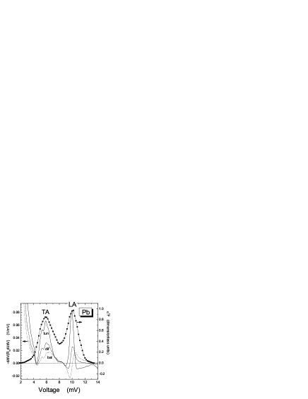
Figure 1: The second derivative of $I-V$ characteristics for superconducting lead $S-c-N$ point contact calculated by Eqs. (8), (7), (6) for the tunnel (solid curve), diffusive (dash-dotted curve) and ballistic (dotted curve) regimes of current flow. $\Re\Delta\left(\varepsilon\right)$ and $\Im\Delta\left(\varepsilon\right)$ are taken from the Rowell-McMillan-Dynes RowDyn tabulation. Squared symbols stand for Rowell-McMillan-Dynes RowDyn EPI spectral function shifted by $\Delta=1.4$ meV to the right on the voltage scale. Its ordinate scale is shown on the right side.

Comparing the exact spectra (Eqs. (6), (7), (8)) with the asymptotic ones (Eqs. (9), (10), (11)), we see that for Pb the differences are only minor (the example for diffusive point-contact is shown in Fig. 2). It goes without saying that the differences for materials with greater ratios of phonon energy to the energy gap, $\hbar\omega_{ph}/\Delta$, will be very small. For example, in Sn or MgB₂ , where $\hbar\omega_{ph}/\Delta\gg 1$ the differences between exact and asymptotic curves in the phonon energy range become indistinguishable.

Figure 2: Comparison of the exact (7) and asymptotic (10) calculated curves for lead in the $S-c-N$ point contact.

Experimentally, the expected shift of the Pb phonon spectra to the right was first noticed in Ref. Khot, . Unfortunately, in this paper (and also in the review paper Yan2000 ) the experimental curves were compared with theoretical ones without allowing for the shift of the latter by $\Delta$ to the right. In Fig. 3 this drawback is corrected and the important consequences are drawn for the ballistic point contact. The upper panel of Fig. 3 displays two experimentally recorded dependences: i) the second derivative of the $I\_V$ characteristic in the normal state (superconductivity is destroyed by the magnetic field) and ii) the same dependence in the superconducting state. The BCS dependence in the superconducting state is shown for comparison. The theoretically expected point-contact spectrum for ballistic contact is shown in the bottom panel of Fig. 3. It is compared with the experimental PC EPI spectrum in the normal state shifted by $\Delta_{Pb}=1.4$ meV . As expected, the position of the calculated TA-maximum coincides with the TA-maximum in the normal-state spectrum and the corresponding feature (zero of $y$-coordinate) coincides with the normal-state LA-maximum (see Fig. 1).

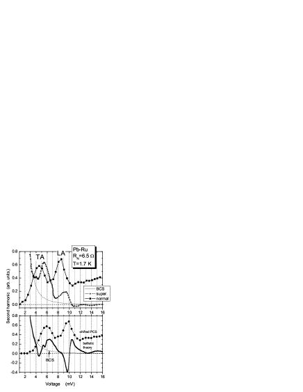
Figure 3: The Pb-Ru experimental point-contact spectra in the normal (squared symbols) and superconducting (triangles-up) states (upper panel) Khot . The calculated spectrum for a ballistic point contact is shown in the lower panel (triangles-down) together with the experimental PC EPI spectrum shifted by $\Delta=1.4$ meV to the right. The theoretical BCS dependence is shown for comparison (thin dotted curve).

In contrast, the phonon features on the experimental curve in the superconducting state shown in the upper panel are noticeably displaced to the left from the expected calculated positions (shown in the lower panel) towards the non-shifted phonon maxima. This displacement is the result of mixing at least of two different mechanisms of revealing the phonon features: namely, the inelastic backscattering current, which has the same positions both in the superconducting and the normal states (the latter is shown as an experimental PC EPI curve in upper panel of Fig. 3), and the theoretical zeroth-order approximation of excess current shown as a theoretical curve in the lower panel. Such mixing seriously impedes interpretation of PC spectra of a ballistic strong-coupling superconductor. Fortunately, as mentioned above, in diffusive point contact the inelastic backscattering current is negligible and the pure self-energy effect on excess current becomes clearly visible. The latter situation holds in MgB₂ films measured along the $c$-direction as well.

III Self-energy effect in $c$-axis oriented MgB₂ films

For two-band superconductor MgB₂ (see the review MazAnt ) the $\Re\Delta\left(\omega\right)$ and $\Im\Delta\left(\omega\right)$ for $\pi$ and $\sigma$-band are depicted in the upper and lower panel of Fig. 4 Yan2004 , respectively. We are interested mostly in the $\pi$-band dependences, since for thin films oriented along the $c$-axis only the $\pi-$band part of the Fermi surface has nonzero Fermi velocity for charge carriers (holes) along the contact axis, playing the main role in the contact current. For the $\sigma$-band, which is two-dimensional, only holes with the velocity in the $ab$-plane exist. The driving force for superconductivity is the very strong EPI of these holes with the $E_{2g}$-phonon mode with the energy of about 70 meV. This mode is seen as the strong peak in $\Re\Delta_{\sigma}$ in the lower panel of Fig. 4 MazAnt . Note, that the ordinate scale for the latter panel is about three times higher than that for the $\pi$-band. For the $\pi-$band all the phonons in the energy range $\sim 30\pm 100$ meV take part in the $\Re\Delta_{\pi}$ dependence, but with a lower magnitude as compared with the $\sigma$-band. Up to about 80 meV $\Im\Delta\left(\omega\right)$ is small, hence, only $\Re\Delta\left(\omega\right)$ is important in Eqs. (9), (10), (11). Thus, we expect that up to $\sim 80$ meV the point-contact spectra differ only in amplitude just like the prefactors in the $\left[\Re\Delta\left(\varepsilon\right)/\varepsilon\right]^{2}$ term. This is evident from Fig. 5.

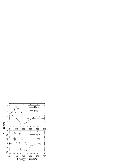
Figure 4: Real and imaginary parts of $\Delta\left(\varepsilon\right)$-dependences for $\pi$- and $\sigma$-bands (upper and lower panels, respectively) of MgB₂ Yan2004 .

We can see that up to the energies $\sim 80\div 90$ meV the shapes of the calculated spectra are similar (Fig. 5). The discrepancy is observed only at higher energies, where $\Im\Delta\left(\omega\right)$ becomes essential. In the range of biases 80$\div$120 meV the variations of point-contact spectra are quite appreciable and mirror in the experimental curves. Although the $\Delta\left(\omega\right)$ value is of the order of $\Delta_{\max}$ at biases higher than 120 meV, the phonon features on the PC spectra are small enough, due to the factor $1/\varepsilon^{2}\left(\omega\right)$. When we compare theoretical and experimental curves, we consider only the biases up to 120 meV, since for higher biases the experimental results are irreproducible, due to nonequilibrium suppression of the superconducting state in the contact.

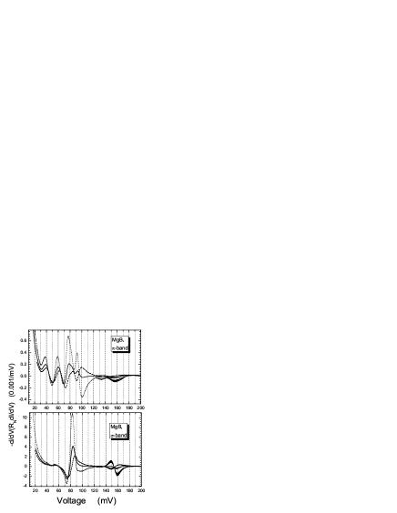
Figure 5: Calculated point-contact spectra for $\pi$- and $\sigma$-bands (upper and lower panels, respectively) of MgB₂ Yan2004 for ballistic (dashed curve), diffusive (thick solid curve) and tunnel (dotted curve) regimes of current flow. Real and imaginary parts of $\Delta\left(\varepsilon\right)$ are taken from Fig. 4.

Comparison of calculated and experimental curves is shown in Fig. 6. For the ordinate scale we use the second harmonic voltage $V_{2}$ measured in experiment, which is related to the second derivative of the $I-V$ characteristic as follows:

$$V_{2}(V)=-\frac{V_{1}^{2}}{2\sqrt{2}}\frac{d}{dV}\left(R_{N}\frac{dI}{dV}\right),$$ (12)

where $V_{1}$ is the modulation voltage, which is conventionally taken equal to 3 meV (close to the value used in the experiment).

In the upper panel of Fig. 6 three different point-contact spectra are shown. They have similar shape up to 100 meV with a slight increase of average amplitudes in the row $R_{N}=$ 49$\rightarrow$36$\rightarrow$80 $\Omega$. In the same sequence the so-called zero-bias maximum in the $dV/dI(V)$ characteristic increases (not shown) , being $R_{0}/R_{N}\leq 1$, $\simeq 1$ and $\geq 1$, respectively ($R_{0}$ is the zero-bias resistance in the superconducting state), for the above mentioned row. One may speculate that in the same direction the contact changes from ballistic towards the tunnel regime. The lower panel of Fig. 6 shows that in the same row the average amplitude of phonon structure increases in the calculated curves.

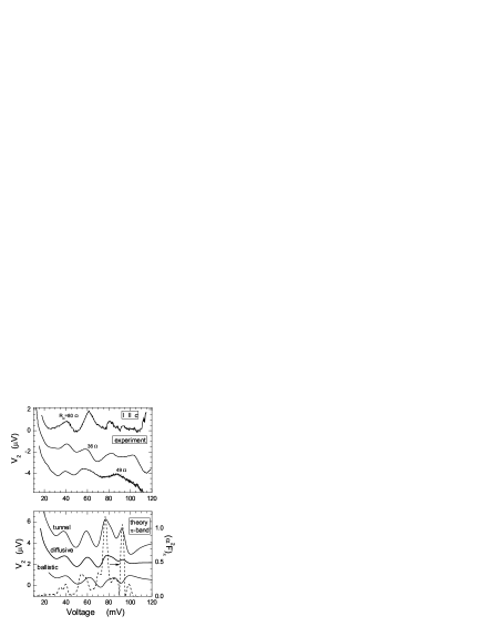
Figure 6: Comparison of experimental (upper panel) and calculated (lower panel) phonon structures in point-contact spectra of MgB₂. The contact axis is oriented along the $c$-axis. The normal state resistances are given for each curve. In the experimental panel the upper curve corresponds to the ordinate scale, and the other two are shifted down for clarity. $T=4.2$ K. In the theoretical (lower) panel three transport regimes are illustrated on the same scale as in the experimental graph. Here, the lower curve corresponds to the ordinate scale, the other two are shifted up for clarity. The $\pi$-band EPI function (dashed curve) Gol is shifted to higher voltages by $\Delta_{\pi}=2.4$ meV. The modulation voltage is taken equal to 3 mV.

The positions of the maxima of the experimental phonon features roughly correspond to the expected ones taking into account that the orientation of experimental junction is approximately along the $c$-axis, since the spreading behavior of current in direct conductivity point contact embraces a wide solid angle near the contact axis. The alignment of our contacts along the $c$-axis is inferred indirectly by measuring the Andreev reflection spectra in the energy gap region and by observation of only the small gap $\Delta\approx 2.4$ meV characteristic of the $\pi$-band.

Special attention should be paid to the amplitude of the experimental curves, which roughly equals that predicted theoretically. In inelastic spectroscopy the amplitude of the EPI spectrum is an order of magnitude lower than expected one (see Fig. 4 in Ref. Bob, and the discussion cited therein). This discrepancy may be explained either by the diffusive regime of current flow with and unknown mean free path $l_{i}$, or by the specific PC-transport character of the EPI function obtained from the inelastic backscattering spectrum.

Comparing theoretical and experimental spectra, one can infer that all the phonons are essential in the EPI function for the $\pi$-band. In the lower panel of Fig. 6 we plot the $\left(\alpha^{2}F\right)_{\pi}$ function taken from Ref. Gol, . As expected, the maxima in the EPI spectral function shifted by $\Delta_{\pi}(0)$ to the right coincide approximately with the maxima in the second harmonic dependences $V_{2}(V)$.

IV Conclusion

The self-energy effect in the phonon feature of a superconducting point contact can be used, in principle, in the same way as the Rowell-McMillan program for determination of the EPI spectral function in tunneling spectroscopy of superconductors RowMcM . Two difficulties arise on this way. One is theoretical, since this program works well only for the one-band superconductor, and its application to the two-band case, like MgB₂, encounters difficulties Shulga . The other is experimental, since all other sources of $I-V$ nonlinearities should be removed, and especially, the nonequilibrium effects in superconductor should be excluded.

The result obtained for superconductivity in MgB₂ is the first direct proof of validity of the calculated EPI function Gol , at least in the $\pi$-band. Unfortunately, this method encounters difficulty, while applying it to the $\sigma$-band. In this case the very strong generation of nonequilibrium phonons cannot be efficiently excluded from the contact region and this destroys the superconductivity in the constriction.

The question may arise whether the self-energy effects are important in the normal state. These are known to be smaller than the inelastic backscattering nonlinearities in the ballistic regime Jan . If we decrease the contact size $d$ or the elastic mean free path $l_{i}$ in order to make the inelastic contribution negligible, the latter parameters become comparable to the Fermi wave length of charge carriers and the strong nonlinearities connected with localization occur, which masks the desired phonon structure Yanloc .

V Acknowledgements

The author is grateful to Yu.G. Naidyuk, S.I. Beloborod’ko, O.V. Dolgov and A.A. Golubov for collaboration. The paper is a review talk at Miami NATO Advanced Research Workshop on New Challenges in Superconductivity in January, 2004. The work was carried out in part by the State Foundation of Fundamental Research under Grant $\Phi$7/528-2001.

References

- (1) I.O. Kulik, A.N. Omel’yanchuk and R.I. Shekhter, Sov. J. Low Temp. Phys. 3, 840 (1977).
- (2) I.K. Yanson, in book ”Quantum Mesoscopic Phenomena and Mesoscopic Devices in Microelectronics”, I.O. Kulik and R. Ellialtioğlu (eds.), p. 61, (2000 ) Kluwer Academic Publishers.
- (3) I.O. Kulik and I.K. Yanson, Sov. J. Low Temp. Phys. 4, 596 (1978).
- (4) I.O. Kulik, R.I. Shekhter and A.G. Shkorbatov, Sov. Phys. JETP 54, 1130 (1981).
- (5) Yu. V. Sharvin, Sov. Phys. JETP 21, 655 (1965).
- (6) V.A. Khlus and A.N. Omel’yanchuk , Sov. J. Low Temp. Phys. 9, 189 (1983).
- (7) V.A. Khlus, Sov. J. Low Temp. Phys. 9, 510 (1983).
- (8) S.N. Artemenko, A.F. Volkov and A.V. Zaitsev, Solid State Commun. 30, 771 (1979).
- (9) G.E. Blonder, M. Tinkham and T.M. Klapwijk, Phys. Rev. B 25, 4515 (1982).
- (10) A.N. Omel’yanchuk, S.I. Beloborod’ko and V.A. Khlus, Sov. J. Low Temp. Phys. 14, 630 (1988).
- (11) S.I. Beloborod’ko and A.N. Omel’yanchuk, Sov. J. Low Temp. Phys. 14, No.3, (1988).
- (12) I.K. Yanson, S.I. Beloborod’ko. Yu.G. Naidyuk, O.V. Dolgov and A.A. Golubov, Phys. Rev. B (Rapid Communication), to be published (2004).
- (13) J.M. Rowell, W.L. McMillan and R.C. Dynes, Bell Laboratories Preprint II, 145 pages, (1969).
- (14) A.V. Khotkevich, V.V. Khotkevich, I.K. Yanson and G.B. Kamarchuk, Sov. J. Low Temp. Phys. 16, 693 (1990).
- (15) I.I. Mazin and V.P. Antropov, Physica C 385, 49 (2003).
- (16) N.L. Bobrov, P.N. Chubov, Yu.G. Naidyuk, L.V. Tyutrina, I.K. Yanson, W.N. Kang, H.-J. Kim, E.-M. Choi, and S.-I. Lee, in book ”New Trends in Superconductivity”, J.F. Annett and S. Kruchinin (eds.), p. 225 (2002) Kluwer Academic Publishers.
- (17) A.A. Golubov, J. Kortus, O.V. Dolgov, O. Jepsen, Y. Kong, O.K. Andersen, B. Gibson, K. Ahn, and R.K. Kremer, J. Phys.: Condens. Matter 14 1353 (2002).
- (18) E.L. Wolf, ”Principles of electron tunneling spectroscopy”, Oxford University Press, Inc. New York.
- (19) O.V. Dolgov, R.S. Gonnelli, G.A. Ummarino, A.A. Golubov, S.V. Shulga, and J. Kortus, Phys. Rev. B 68, 132503 (2003).
- (20) A.G.M. Jansen, A.P. van Gelder and P. Wyder, J. Phys. C 13, 6073 (1980).
- (21) I.K. Yanson, O.I. Shklyarevskii and N.N. Gribov, J. Low Temp. Phys. 88, 135 (1992).