dc-Response of a Dissipative Driven Mesoscopic Ring.

Abstract

The behavior of the dc-component of the current along a quantum loop of tight-binding electrons threaded by a magnetic flux that varies linearly in time $\Phi_{M}(t)=\Phi t$ is investigated. We analize the electron transport in different kinds of one-dimensional structures bended into a ring geometry: a clean one-dimensional metal, a chain with a two-band structure and a disordered chain. Inelastic scattering events are introduced through the coupling to a particle reservoir. We use a theoretical treatment based in Baym-Kadanoff-Keldysh non-equilibrium Green functions, which allows us to solve the problem exactly.

I Introduction

The impressive development of nanoscience places the detailed understanding of quantum transport in mesoscopic systems among the main challenges of condensed matter physics. A rich variety of devices and structures, including simple metallic wires, as well as complex molecules, where electrons are driven by some external force, are the subject of experimental and theoretical investigation. The driving field can be established by attached leads at different chemical potentials, a magnetic flux when the system is bended into a ring or time-dependent fields. Transport properties, like the conductance of the system, depend strongly on its microscopic details but they may also depend on the underlying driving mechanism.

A simple quasi one-dimensional annular system threaded by a magnetic flux is one of the paradigmatic devices to discuss the fundamentals of quantum effects dominating the electron transport. Several outstanding experiments ab1 ; ab11 ; ab12 and theoretical works ab2 ; imb have been devoted to the investigation of phenomena related to the Aharanov-Bohm effect in rings enclosing a static magnetic field. There is, however, relatively less literature related to the case where the field changes in time. Among the latter category of problems, a very interesting example corresponds to that of a magnetic flux with a linear dependence on time: $\Phi_{M}(t)=\Phi t$, which induces a constant electric field along the ring.

This problem was discussed by Büttiker, Imry and Landauer in the early times of the theory of quantum transport ibl . Their motivation was to search alternative schemes to calculate the conductance of a system to that proposed by Landauer lan , where the sample is placed between two reservoirs at different chemical potentials. As first discussed in that seminal work, such device isolated from the external world, is not appropriate to observe a dc-current since the electrons inside move coherently displaying Bloch oscillations and producing a pure ac-response. In a subsequent work Landauer and Büttiker bl showed that when a dissipative mechanism is added to that system a dc-current is established. Büttiker also showed that a concrete element to introduce inelastic scattering events and dissipation is a lead connecting the loop to a particle reservoir but . Soon later, Lenstra and van Haeringen suggested that a dc-current can be generated in that device by elastic scattering introduced by weak disorder lh . The possibility of “resistive” behavior originated in pure elastic scattering processes generated a series of interesting discussions and criticisms lan1 ; lan2 ; gef1 ; gef2 ; brou ; ao ; av . Most of the ideas of these works are based on adiabatic descriptions where the energy levels of the ring define minibands in a parametric representation as periodic functions of the flux. Within that adiabatic framework, scattering processes form small gaps between the so defined minibands while the time dependence of the field gives rise to Zener tunneling across them. In Refs. gef1 ; gef2 interesting arguments emphasizing the concept of localization in the energy space as a consequence of disorder have been proposed against the possibility of dc-response without dissipation.

The discussion of the role of dissipative effects in the driven ring was introduced on the basis of a phenomenological equation of motion that describes the relaxation via inelastic scattering processes (ISP) of the time-dependent occupation of a miniband bl . The main argument was that the dc-response should vanish in the limit of vanishing and strong relaxation, while it should peak at some intermediate regime. For small electric fields, the behavior of the current is also found to follow a linear, ie. Ohmic-like, dependence as a function of the induced electromotive force (emf). These notable predictions have not been examined in more detail during many years. Quite recently, the effect of inelastic scattering in the dc-behavior of that system has been studied liu . In that work a pure “clean” system is considered, (ie without any kind of elastic scattering). Non-Ohmic behavior has been found in the dc-current vs emf characteristic curve within the limit of small ISP, while the dc-current is found to decrease continuously as the strength of the ISP increases. The fact that no tendency towards a vanishing component of the dc-current is observed as the dissipation tends to be suppressed is rather surprising, since the limit of pure Bloch oscillations in the isolated system seems not to be recovered.

In this work we consider a ring threaded by a flux with a linear time dependence and we analyze in detail the role of dissipation in that system. We study the clean one-band system as well as the effect of two different kinds of elastic scattering processes: a periodic potential with a two-sublattice profile and a random potential. The effect of inelastic scattering is modeled by means of the coupling to a particle reservoir through an external lead. We use a recently proposed theoretical treatment based on Baym-Kadanoff-Keldysh Green functions lili which enables a full out-of-equilibrium description of the time-dependent problem, without introducing any kind of adiabatic assumptions or approximations. As far as no many-body interactions are considered, that treatment leads to the exact solution of this problem. Thus, one of the aims of this work is to analyze the case of the disordered driven ring in the limit of weak ISP, which has focused several efforts but has never been tackled with an exact method. The formalism based on Green functions is particularly appealing to deal with the coupling to external leads and reservoirs. These elements can be introduced by means of physical models and they can be concisely represented by self-energies, avoiding further assumptions about the boundary conditions. We consider two different electronic models for the lead: one is described by a constant density of states and a very wide band, while the other is represented by a semi-infinite tight-binding chain. We show that the dc-response does not depend qualitatively on the latter details. In all the cases, our results indicate that the dc-current tends to a vanishing value as the coupling to the reservoir goes to zero, displays a maximum and then decreases as that coupling becomes stronger. For clean systems, the position of the maximum shifts towards very low ISP strengths as the emf decreases and as the length of the ring increases.

The system considered here, actually lies in the category of the so called ratchet problems, since the induced electric field by itself is not able to produce a dc-response, needing the aid of some additional rectification mechanism. This motivates the analysis of the transport properties of this system in the framework of recent symmetry arguments proposed to examine rectification processes in ratchet systems in the presence of time-periodic fields ser1 ; ser2 ; ser3 . Such arguments provide further support to the idea that dissipation is an essential ingredient for this system to have a dc-current irrespectively the particular nature of the elastic scattering along its circumference.

The paper is organized as follows. In section II we present the model and the theoretical approach to analyze the behavior of the current. In section III we present the results. Section IV is devoted to summary and conclusions.

II Theoretical treatment

II.1 The model

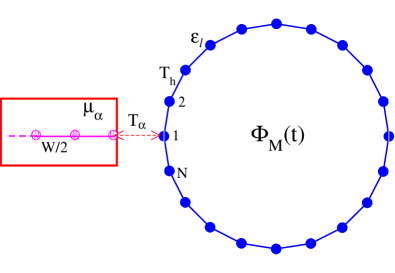
Figure 1: (Color on line) Scheme of the setup. The system indicated in the red box defines the reservoir with chemical potential $\mu_{\alpha}$.

We consider the device sketched in Fig. 1. It consists in a ring threaded by a magnetic flux with a dependence on time of the form $\Phi_{M}(t)=\Phi t$, in contact to a particle reservoir with a chemical potential $\mu_{\alpha}$ through an external lead. The full system is described by the following Hamiltonian:

$$H=H_{ring}(t)+H_{\alpha}+H_{1\alpha},$$ (1)

where the first term, representing the ring, depends explicitly on time due to the presence of the time-dependent flux. We consider noninteracting spinless electrons described by a tight binding model with $N$ sites and lattice constant $a=L/N$. We also consider the possibility of elastic scattering in the system, described by a local energy with a profile $\epsilon_{l}$ with $l=1,\ldots,N$. The Hamiltonian is

$$H_{ring}=-T_{h}\sum_{l=1}^{N}(e^{-i\phi t}c^{\dagger}_{l}c_{l+1}+e^{i\phi t}c^{\dagger}_{l+1}c_{l})+\sum_{l=1}^{N}\epsilon_{l}c^{\dagger}_{l}c_{l},$$ (2)

with the periodic condition $N+1\equiv 1$. The time-dependent phase $\phi t$ attached to each link, with $\phi=\Phi/(\Phi_{0}N)$, being $\Phi_{0}=hc/e$, accounts for the presence of the external magnetic flux.

The term $H_{\alpha}$ describes the reservoir. We consider two models of noninteracting electrons with a bandwidth $W$ and a chemical potential $\mu_{\alpha}$ for this system: (i) a wide-band model, defined by a constant density of states and a very large $W$, and (ii) a semi-infinite tight binding chain with hopping amplitude $W/2$, which corresponds to a semicircular density of states $\rho_{\alpha}(\omega)=4\Theta(|\omega|-W)\sqrt{W^{2}-\omega^{2}}/W^{2}$.

The last term of $H$,

$$H_{1\alpha}=-T_{\alpha}(c^{\dagger}_{1}c_{\alpha}+c^{\dagger}_{\alpha}c_{1}),$$ (3)

represents the connection between the ring and the reservoir.

II.2 Dynamical equations and symmetry properties

In Refs. ser1 ; ser2 ; ser3 an interesting connection has been suggested between the rectification properties of the system and the underlying symmetries of the equations of motion in several ratchet problems. The main idea is that the symmetries of the equation of motion that change the sign of the velocity would lead to a vanishing dc-component of the current. We now turn to follow the lines suggested in those works to carry out a similar symmetry analysis in our problem.

Let us first consider the simpler case of the ring isolated from the reservoir, the problem is described by $H_{ring}$ alone. For sake of simplicity in the notation we shall adopt a system of units where $\Phi_{0}=1,\;\hbar=1$. The relevant equation of motion is the Schrödinger equation

$$-i\frac{\partial}{\partial t}\psi_{l}(t)=\varepsilon_{lk}(t)\psi_{k}(t),$$ (4)

being $\varepsilon_{lk}(t)=-T_{h}(e^{-i\phi t}\delta_{k,l+1}+e^{i\phi t}\delta_{k,l-1})$. We have adopted the Einstein summation rule over site indexes. The current in the isolated ring results

$$J^{isol}_{l,l+1}(t)=eT_{h}\mbox{Im}[e^{-i\phi t}\psi^{*}_{l}(t)\psi_{l+1}(t)].$$ (5)

The matrix elements of the Hamiltonian satisfy

$$\varepsilon_{lk}^{*}(-t)=\varepsilon_{lk}(t)=\varepsilon^{*}_{kl}(t).$$ (6)

Hence, the inversion $t\rightarrow-t$ followed by the complex conjugation of (4) leads to $\psi^{*}_{l}(-t)=\psi_{l}(t)$ which, when replaced in (5), results in the following property of the current

$$J^{isol}_{l,l+1}(-t)=-J^{isol}_{l,l+1}(t).$$ (7)

Since in our reasoning we have not assumed any particular form for the energy profile $\epsilon_{l}$, the criterion of Refs. ser1 ; ser2 ; ser3 rules out the possibility of a dc-current as far as time-reversal symmetry is preserved in the device irrespectively the particular model assumed for the elastic scattering processes. Another symmetry operation that changes the sign of the current is spatial reflection, however, the latter is not a symmetry of the Schrödinger equation (4).

In the more general case, when inelastic scattering processes are considered, the relevant equation of motion is the Dyson equation for the Green function. In the framework of Baym-Kadanoff-Keldysh formalism the latter has a matrix form and one must work with two independent Green functions: the retarded Green function,

$$G^{R}_{i,j}(t,t^{\prime})=-i\Theta(t-t^{\prime})\langle[c_{i}(t),c^{\dagger}_{j}(t^{\prime})]\rangle,$$ (8)

and the lesser Green function

$$G^{<}_{i,j}(t,t^{\prime})=i\langle c^{\dagger}_{j}(t^{\prime})c_{i}(t)\rangle.$$ (9)

The latter determines the mean values of the observables. In particular, the current through a bond $\langle l,l+1\rangle$ is written as

$$J_{l,l+1}(t)=2eRe[T_{h}e^{-i\phi t}G^{<}_{l+1,l}(t,t)].$$ (10)

The Dyson equation for the matricial Green function leads to the equations of motion for the retarded and lesser components ram

$$-i\frac{\partial}{\partial t^{\prime}}G^{R}_{ij}(t,t^{\prime})-G^{R}_{ik}(t,t^{\prime})\varepsilon_{kj}(t^{\prime})=\delta(t-t^{\prime})\delta_{ij}$$

$$+\int dt^{\prime\prime}\,G^{R}_{ik}(t,t^{\prime\prime})\Sigma^{R}_{kj}(t^{\prime\prime},t^{\prime}),$$

$$-i\frac{\partial}{\partial t^{\prime}}G^{<}_{ij}(t,t^{\prime})-G^{<}_{ik}(t,t^{\prime})\varepsilon_{kj}(t^{\prime})=$$

$$\int dt^{\prime\prime}[G^{R}_{ik}(t,t^{\prime\prime})\Sigma^{<}_{kj}(t^{\prime\prime},t^{\prime})$$

$$+G^{<}_{ik}(t,t^{\prime\prime})\Sigma^{A}_{kj}(t^{\prime\prime},t^{\prime})]\;,$$ (11)

while the evolution for the lesser component at equal times is given by

$$i\,\frac{dG^{<}_{ij}(t,t)}{dt}-G^{<}_{ik}(t,t)\varepsilon_{kj}(t)+\varepsilon_{ik}(t)G^{<}_{kj}(t,t)$$

$$=\int dt^{\prime\prime}\;[\;\Sigma^{R}_{ik}(t,t^{\prime\prime})G^{<}_{kj}(t^{\prime\prime},t)+\Sigma^{<}_{ik}(t,t^{\prime\prime})G^{A}_{kj}(t^{\prime\prime},t)$$

$$-G^{R}_{ik}(t,t^{\prime\prime})\Sigma^{<}_{kj}(t^{\prime\prime},t)-G^{<}_{ik}(t,t^{\prime\prime})\Sigma^{A}_{kj}(t^{\prime\prime},t)\;]\;,$$ (12)

being $G^{A}_{i,j}(t,t^{\prime})=[G^{R}_{j,i}(t^{\prime},t)]^{*}$ and $\Sigma^{A}_{i,j}(t,t^{\prime})=[\Sigma^{R}_{j,i}(t^{\prime},t)]^{*}$.

In the Hamiltonian limit, $\Sigma^{R}_{i,j}(t,t^{\prime})=\Sigma^{<}_{i,j}(t,t^{\prime})\equiv 0$, in the absence of many-body interactions. Making use of the property of the matrix elements of the Hamiltonian (6) and of the symmetry property of the Green function $G^{<}_{j,i}(t,t^{\prime})=-[G^{<}_{i,j}(t^{\prime},t)]^{*}$, the property (7) for the time-inversion operation on the current is recovered.

It is easy to verify that any non-vanishing self-energy correction that fails to satisfy the properties $\Sigma^{<}_{ik}(t,t^{\prime})=\Sigma^{>}_{ik}(t,t^{\prime})\equiv 0$, $\Sigma^{R}_{ik}(t,t^{\prime})=s_{ik}(t)\delta(t-t^{\prime})$, with $s_{ij}(t)=s^{*}_{ji}(t)=s_{ji}(-t)$, breaks time-reversal symmetry in the equations of motion. In particular, any self-energy represented by kernels of the form

$$\Sigma^{R}_{ik}(t,t^{\prime}) = -i\Theta(t-t^{\prime})\int\frac{d\omega}{2\pi}\{-2\mbox{Im}[\Sigma^{R}_{ik}(\omega)]\}e^{-i\omega(t-t^{\prime})},$$

$$\Sigma^{<}_{ik}(t,t^{\prime}) = i\int\frac{d\omega}{2\pi}f(\omega)\{-2\mbox{Im}[\Sigma^{R}_{ik}(\omega)]\}e^{-i\omega(t-t^{\prime})},$$ (13)

with $\mbox{Im}[\Sigma^{R}_{ik}(\omega)]\neq 0$, being $f(\omega)$ the Fermi function, will break time-reversal symmetry in the equations of motion for the Green functions and will break the property (7) for the time-dependent current.

In our problem, the effect of the exchange of particles and energy between the mesoscopic system and the reservoir can be exactly written in terms of a self-energy correction at the site $l=1$ of the tight-binding ring lili ; jau ; past . The retarded and lesser components of this self-energy are

$$\Sigma^{R}_{ik}(t-t^{\prime}) = \delta_{i,1}\delta_{k,1}\Sigma_{1}^{R}(t-t^{\prime})$$

$$= -i\Theta(t-t^{\prime})|T_{\alpha}|^{2}$$

$$\times\int\frac{d\omega}{2\pi}\rho_{\alpha}(\omega)e^{-i\omega(t-t^{\prime})}\delta_{i,1}\delta_{k,1},$$

$$\Sigma^{<}_{ik}(t-t^{\prime}) = \delta_{i,1}\delta_{k,1}\Sigma_{1}^{<}(t-t^{\prime})$$

$$= i|T_{\alpha}|^{2}\int\frac{d\omega}{2\pi}f(\omega)\rho_{\alpha}(\omega)e^{-i\omega(t-t^{\prime})}\delta_{i,1}\delta_{k,1},$$

where $\rho_{\alpha}(\omega)$ is the density of states of the reservoir and the Fermi function is $f(\omega)=1/(e^{\beta(\omega-\mu_{\alpha})}+1)$. In our calculations we consider zero temperature, i.e. $f(\omega)=\Theta(\omega-\mu_{\alpha})$. The wide-band model leads to a constant imaginary retarded self-energy, $\Sigma_{1}^{R}(\omega)=i\sigma$, and $\Sigma_{1}^{<}(\omega)=if_{\alpha}(\omega)\sigma$, being $\sigma=|T_{\alpha}|^{2}\pi/W$. The dissipative nature of the coupling to the reservoir manifests itself in the fact that $\Sigma_{1}^{R}(\omega)$ has a finite imaginary part. As discussed above, this breaks time-inversion symmetry in the dynamical equation, removing the inversion of the current under this symmetry operation. This satisfies the criterion of Refs. ser1 ; ser2 ; ser3 , namely, a non-vanishing net current is possible when symmetries of the equation of motion leading to an inversion of the time-dependent current are broken.

II.3 Evaluation of the Green functions and the dc-current.

The formalism leading to the evaluation of the current along the ring has been presented in Ref. lili . In this subsection we summarize the main equations and we defer the reader to this work and references therein for further details.

Following Ref.lili , it is convenient to perform a gauge transformation in the fermionic operators of the Hamiltonian (2),

$$c_{n}=\exp[in\phi t]\overline{c}_{n},$$ (15)

according to which the Green function for the positions $m,n$ on the ring transforms as

$$G^{R}_{m,n}(t,t^{\prime})=\exp[i\phi(mt-nt^{\prime})]\overline{G}^{R}_{m,n}(t,t^{\prime}).$$ (16)

Defining the Fourier transform

$$G^{R}_{m,n}(t,t^{\prime})=\int\frac{d\omega}{2\pi}G^{R}_{m,n}(t,\omega)e^{-i\omega(t-t^{\prime})},$$ (17)

the resulting equation for the retarded Green function is

$$\overline{G}^{R}_{m,n}(t,\omega) = G^{0}_{m,n}(\omega)-\overline{G}^{R}_{m,N}(t,\omega+\Phi)T_{N1}(t)G^{0}_{1,n}(\omega)$$ (18)

$$-\overline{G}^{R}_{m,1}(t,\omega-\Phi)T_{1N}(t)G^{0}_{N,n}(\omega),$$

with

$$\overline{G}^{R}_{m,1}(t,\omega)+\overline{G}^{R}_{m,N}(t,\omega+\Phi)T_{N1}(t)G^{0}_{1,1}(\omega)$$

$$+\overline{G}^{R}_{m,1}(t,\omega-\Phi)T_{1N}(t)G^{0}_{N,1}(\omega)=G^{0}_{m,1}(\omega)$$

$$\overline{G}^{R}_{m,N}(t,\omega)+\overline{G}^{R}_{m,N}(t,\omega+\Phi)T_{N1}(t)G^{0}_{1,N}(\omega)$$

$$+\overline{G}^{R}_{m,1}(t,\omega-\Phi)T_{1N}(t)G^{0}_{N,N}(\omega)=G^{0}_{m,N}(\omega),$$ (19)

where $T_{1N}(t)=[T_{N1}(t)]^{*}=T_{h}e^{i\Phi t}$. For each time $t$, the solution of the above set of linear equations provides the complete exact solution of the problem.

The equilibrium Green function $G^{0}_{m,n}(\omega)$ corresponds to the problem of an open chain in contact to the reservoir. It is obtained from the solution of the Dyson equation

$$G^{0}_{m,n}(\omega)=g^{0}_{m,n}(\omega)+G^{0}_{m,1}(\omega)\Sigma^{R}_{1}(\omega)g^{0}_{1,n}(\omega),$$ (20)

where

$$g^{0}_{m,n}(\omega)=\sum_{\nu=1}^{N}A^{\nu}_{m}A^{\nu}_{n}\frac{1}{\omega-E_{\nu}+i\eta}$$ (21)

is the Green function of the chain isolated from the reservoir. It can be expressed in terms of the eigenvalues $E_{\nu}$ and eigenvectors $|\nu\rangle=\sum_{l}A^{\nu}_{l}|l\rangle$ of the Hamiltonian

$$\overline{H}_{0}=-T_{h}\sum_{l=1}^{N-1}(\overline{c}^{\dagger}_{l}\overline{c}_{l+1}+\overline{c}^{\dagger}_{l+1}\overline{c}_{l})+\sum_{l=1}^{N}(V_{l}+\epsilon_{l})\overline{c}^{\dagger}_{l}\overline{c}_{l},$$ (22)

where $V_{l}=\phi l$ is the scalar potential due to the induced electric field.

The set (18) and (19) describes the process of the closing of the biased chain by means of an effective time-dependent hopping $T_{1N}(t)$ that pumps electrons with a frequency $\Phi$ through the bond $\langle 1N\rangle$. This set involves, in principle, an infinite number of equations. In the numerical procedure, upper and lower energy cutoffs $\Lambda_{1},\Lambda_{2}$ are chosen such that $\Lambda_{1}<E_{\nu}<\Lambda_{2},\;\forall\nu$.

Starting from its definition (10), the current along the ring can be written

$$J_{l,l+1}(t) = 2eT_{h}\int\frac{d\omega}{2\pi}\mbox{Re}[\Sigma_{1}^{<}(\omega)$$ (23)

$$\times\overline{G}^{R}_{l+1,1}(t,\omega+\phi)[\overline{G}^{R}_{l,1}(t,\omega+\phi)]^{*}],$$

where we have used $G^{A}_{1,l}(t,t^{\prime})=[G^{R}_{l,1}(t^{\prime},t)]^{*}$. Therefore, the evaluation of the time-dependent current is reduced to the evaluation of $\overline{G}^{R}_{l,1}(t,\omega)$ obtained from (19). This quantity displays an oscillatory behavior as a function of $t$, with the period $\tau_{B}=2\pi/\Phi$ of the Bloch oscillations. The dc-component does not depend on the bond $\langle l,l+1\rangle$ chosen for the calculation and it is defined as

$$J_{dc}=\frac{1}{\tau_{B}}\int_{0}^{\tau_{B}}dtJ_{l,l+1}(t).$$ (24)

III Results

This section is devoted to analyze the behavior of the dc-current (24) as a function of the induced emf $\Phi$, the strength of ISP and the chemical potential $\mu_{\alpha}$. The strength of ISP is related to the degree of coupling between the ring and the reservoir. In the case of the wide band model, the parameter $\sigma$ sets that measure. In the model with a semicircular density of states, that measure is given by $T_{\alpha}^{2}/W$. In our calculations, we fixed $W=4T_{h}$ and changed $T_{\alpha}$. All energies will be expressed in units of the hopping parameter $T_{h}$. We shall analize three different energy profiles $\epsilon_{l}$ for the tight-binding model that define a clean one-band chain, a chain with a two-sublattice structure and a random potential.

III.1 The clean one-band ring

This case corresponds to $\epsilon_{l}=0,l=1,\ldots,N$ in (2). In the limit of vanishing dissipation (the ring isolated from the reservoir) the system is described by the Hamiltonian $H_{ring}(t)$ alone, the problem has time-reversal symmetry and a vanishing dc-current is expected. In fact, for $\epsilon_{l}=0$, $H_{ring}(t)$ can be easily solved by performing a Fourier transform to the $k$-space. The retarded Green function can be calculated analytically, resulting $G^{R}_{m,n}(t,t^{\prime})=-i\Theta(t-t^{\prime})\sum_{k}\exp\{ik(m-n)\}\exp\{-i\int_{t}^{t^{\prime}}ds\epsilon_{k}(s)\}$, with $\epsilon_{k}(s)=-2T_{h}\cos(k+\phi s)$, being $k=2n\pi/L,n=0,\ldots,N$. The current can also be obtained analytically, resulting

$$J(t)=T_{h}\sum_{k}\sin(k+\phi t).$$ (25)

where the summation extends over the set of occupied $k$-states.

The behavior of the dc-current in the coupled system at a fixed chemical potential $\mu_{\alpha}$ for different strengths of ISP and $\Phi$ is analyzed in Fig. 2. A wide band model was assumed for the reservoir in these calculations. The dc-current displays a maximum which shifts to lower values of $\sigma$ as $\Phi$ decreases. At low $\sigma$, the imaginary part of $G^{0}_{m,n}(\omega)$ evolve towards a sequence of delta functions and the Green functions $\overline{G}^{R}_{m,n}(t,\omega)$ also develop a structure of peaks that get sharper. From the practical point of view, this turns harder the evaluation of the integral in $\omega$ (23), preventing us from exploring the range of $\sigma/T_{h}<0.05$. However, we think that the range considered is enough to infer the trend towards $\sigma\rightarrow 0$. The characteristic curves $J_{dc}$ vs $\Phi$ are shown in the inset for particular values of $\sigma$ within the regimes with low, intermediate and strong coupling to the reservoir. In the latter limit, the dc-current remains linear within a wide range of $\Phi$ while for weak coupling, the departure from linear response takes place at small $\Phi$.

Figure 2: (Color online) dc-current as a function of $\sigma$ in a ring with $N=20$ sites for different values of the induced electric field $\Phi=0.01,0.02,0.04,0.06,0.08,0.1,0.2,0.3,0.5$ (upper panel) and with $N=200$ for $\Phi=0.2,0.3,0.4,0.5$ (lower panel). The chemical potential of the reservoir is $\mu_{\alpha}=-1$. The plots corresponding to the lowest and the highest $\Phi$ are drawn in white and black symbols, respectively, while grey symbols correspond to intermediate values. Inset: $J_{dc}$ vs $\Phi$ characteristic curve for different strengths of ISP corresponding to $\sigma=0.05,0.2,0.8$ (red circles, green squares and blue diamonds).

To study the origin of this peculiar behavior we must analyze the structure of the equations (18) and (19). At each time $t$, the Green function $\overline{G}^{R}_{m,n}(t,\omega)$ contains a combination of a large number of $\omega$-components (separated in $\Delta\omega=\Phi$) of the Green function (20). In the weak coupling limit, $G^{0}_{m,n}(\omega)$ is sizable only within a neighborhood of the $N$ frequencies $E_{\nu}$. Therefore, a resonant combination of components at different frequencies is achieved when $\Delta\omega\sim\Delta E_{\nu}$, the latter being the mean energy separation between two eigenenergies, $\Delta E_{\nu}=\langle E_{\nu+1}-E_{\nu}\rangle\sim 4T_{h}/N$. Whether such interference will be constructive or destructive and give rise to a large or a small component of the dc-current is a question without obvious answer, particularly in the case of small $\Phi$, where the number of coupled frequencies is very large. On general grounds, one expects that such an effect would strongly depend on the underlying symmetries of the model. Related discussions have been recently presented in problems of pumping introduced by microwave fields leh ; han ; mos where the Floquet representation of the wave function is used, leading to a structure of the solution containing a mixing of frequencies that differ in the frequency of the pumping field. In our problem, it becomes apparent that such interference is constructive regarding the magnitude of $J_{dc}$ and for this reason, in the weak coupling limit, the current grows linearly as a function of $\Phi$, reaching a maximum at $\Phi\sim\Delta E_{\nu}$. The decrease for $\Phi>>\Delta E_{\nu}$ can be understood by noting that the number of resonances is approximately $4T_{h}/\Phi$, becoming smaller as $\Phi$ increases. The maximum of $J_{dc}$ as function of $\sigma$ can be also interpreted in terms of combination of components of the Green function from different frequencies. In fact, the effect of increasing ISP is to spread the spectral weight of the peaks of $G_{m,n}^{0}(\omega)$. Thus, for strong coupling the interference involves a large number of frequencies but with a low (approximately constant) weight. For lower ISP, the amplitudes can be large for frequencies close to $E_{\nu}$ but tend to be vanishingly small in between. The result is that there is a maximum in $J_{dc}$ at some strength of ISP that seems to scale as $\propto\Phi$, at least, within the regime $\Phi>\Delta E_{\nu}$. On the side of strong coupling, where the resonant effects are highly smoothed, the resulting dc-current is relatively smaller (consistent with the idea that resistance increases with ISP) and behaves linearly within a larger range of $\Phi$.

The effect of the length of the chain is also analyzed in Fig.2. The first issue to note is that in the $N=200$ sites ring (see lower panel of Fig. 1, the dc-current for $\Phi=0.2$ remains growing for the smallest $\sigma$ considered. Instead, for $N=20$ and the same parameters, the current decreases down from its maximum (cf upper panel of Fig. 2). This behavior is consistent with the picture of constructive resonances: The condition $\Phi>\Delta E_{\nu}$ is achieved in this case at lower $\Phi$, while the larger number of peaks increases the probability of resonances and the current remains large, within a larger range of $\Phi$. For larger fields and for larger $\sigma$, the qualitative and quantitative behavior is essentially the same as that observed in the smaller ring.

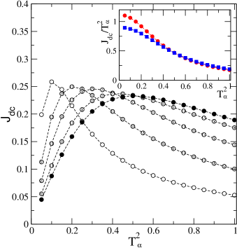
Figure 3: (Color online) dc-current as a function of the strength of ISP for a model with a semicircular density of states with bandwidth $W=4$. Different plots correspond to $\Phi=0.1,0.2,0.3,0.4,0.5$. The plots in white and black symbols correspond to the lowest and the highest $\Phi$, while the grey ones correspond to the intermediate values. The chemical potential of the reservoir is $\mu_{\alpha}=-1$. Inset: Detail of the behavior of $J_{dc}$ for low ISP. Red circles and blue squares correspond to $\Phi=0.4,0.5$, respectively. The behavior is consistent with $J_{dc}\propto T^{2}_{\alpha}$ when $T^{2}_{\alpha}\rightarrow 0.$

Regarding the effect of the model for the reservoir, it becomes clear from the results of Fig. 3 that it does not play any relevant qualitative role since we can identify in these plots the same features observed in Fig. 2. In Ref. leh an interesting connection have been found between the behavior of $J_{dc}$ as a function of $T^{2}_{\alpha}$ when $T^{2}_{\alpha}\rightarrow 0$ and the underlying symmetries of the Hamiltonian. The plots of Fig. 3 corresponding to the two highest emfs ($\Phi=0.4,0.5$), where the decrease to a vanishing $T^{2}_{\alpha}$ can be cleanly captured wihin the shown range of $T^{2}_{\alpha}$, suggest a $J_{dc}\propto T^{2}_{\alpha}$ behavior as $T^{2}_{\alpha}\rightarrow 0$. This is even more clear in the plot of $J_{dc}/T^{2}_{\alpha}$ vs $T^{2}_{\alpha}$ shown in the inset. This dependence can be understood by noting that when $\Delta E_{\nu}+\Phi>>T^{2}_{\alpha}/W$, the retarded Green functions entering the evaluation of $J_{l,l+1}(t)$ (see Eq. 23), can be replaced by the ones for the uncoupled ring (corresponding to $T^{2}_{\alpha}=0$). Hence, for small enough $T^{2}_{\alpha}$, the time-dependent current and also the dc-component $J_{dc}$ become linear in $T^{2}_{\alpha}$. This is in perfect agreement with the analysis done in Ref. leh for a linear device pumped with a laser in configurations with broken time-reversal symmetry.

Figure 4: (Color online) dc-current as a function of the chemical potential of the reservoir (represented by a wide band model) for two values of the emf $\Phi=0.1,0.5$ (solid and dashed lines) and two strengths of ISP $\sigma=0.05,0.85$ (thick black and thin red lines), respectively for a ring with $N=200$ sites.

The behavior of $J_{dc}$ as a function of the chemical potential is shown in Fig.4. It is remarkable that a semicircular shape can be identified in the envelope of these functions. As mentioned before, the density of states of a semi-infinite tight-binding chain of bandwidth $W$, is proportional to a semicircle of radius $W/2$. This motivates the comparison of the conductance of our device with the conductance of a quantum dot which has two semi-infinite tight-binding chains with hopping elements $T_{h}$ and chemical potential $\mu_{\alpha}$ attached to its left and to its right, through a hybridization amplitude $w_{eff}$. The latter corresponds to the usual configuration employed in a Landauer-like calculation of the conductance through a dot connected to a left and a right lead. Assuming that a small bias $V$ is applied between the left and the right, the conductance of such a system is given by a Landauer-like formula miwi

$$G_{eff}=\frac{\partial J_{dc}}{\partial V}=e\rho_{0}(\mu_{\alpha})\Gamma,$$ (26)

where $\rho_{0}(\mu_{\alpha})=\sqrt{4T_{h}^{2}-\mu_{\alpha}^{2}}/T_{h}^{2}$ is the density of states of the semi-infinite chain and $\Gamma=w_{eff}^{2}\rho_{eff}(\mu_{\alpha})/4\pi$, being $\rho_{eff}(\mu_{\alpha})$ the density of states of the central system dressed by the contact with the two chains.

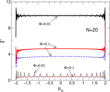
Figure 5: (Color online) $\Gamma$ (proportional to the effective density of states $\rho_{eff}(\mu_{\alpha})$ obtained by assuming a model for the conductance based on a dot coupled to two semi-infinite chains for the case of a ring with $N=20$ sites and a wide band model for the reservoir. Thick and thin solid lines correspond to $\sigma=0.05$ and $\sigma=0.85$, respectively. Black and red lines correspond to $\Phi=0.01$ and $\Phi=0.1$, respectively. The plot in blue dashed lines corresponds to $\Phi=0.1$ and a model of reservoir with a semicircular density of states with $W=4$ and $T_{\alpha}^{2}=0.1$.

In order to define the conductance for the device of Fig. 1, let us note that the induced electric field is $E=\Phi/(Lc)$. Therefore, if we make the standart assumption that for small $\Phi$ the current can be written as $J_{dc}=\sigma_{c}E$, being $\sigma_{c}$ the conductivity, the conductance of the chain is defined from $J_{dc}=GEL$. Therefore, in units where ($c=1$), the conductance for small enough bias is

$$G=\frac{J_{dc}}{\Phi}.$$ (27)

If we adopt the expression (26) as a phenomenological model for the conductance of our system, we obtain for $\Gamma$ the result shown in Fig. 5. In the limit of weak coupling, this behavior is consistent with an effective density of states approximately constant along the band-width. Taking into account its sum rule, it should be $\rho_{eff}(\mu_{\alpha})\sim\Theta(|\mu_{\alpha}|-4T_{h})\pi/4T_{h}$. The large average value of $\Gamma$ indicates a large effective hopping from the dot to the semi-infinite chains ($w_{eff}\sim 12,8$) for $\Phi=0.01,0.1$, respectively. The details of the model used for the reservoir do not influence the final behavior of $\Gamma$. In fact, all the features in the weak coupling regime observed within the wide band model for the reservoir are also obtained with a reservoir with a semicircular density of states (cf plot in dashed lines of Fig. 5). In the strong coupling limit, $w_{eff}\sim 3$ is approximately the same for both fields and a fine structure of $N$ wide peaks is distinguished in $\rho_{eff}(\mu_{\alpha})$. The effective parameters $\Gamma$ and $w_{eff}$ do not have any straightforward significance in the context of our original model and the parallel between the driven ring and the dot connected to semi-infinite chains is purely heuristic. However, it is remarkable the similar behavior of the conductance of the two devices. It suggests that although the chain that forms the ring is made up by a discrete chain with a finite number of sites, the dressing due to the mixing of a large number of frequencies tend to produce a structure such that any site along the ring would feel as if placed between two semi-infinite leads. In spite of this resemblance, the quantitative properties of the conductance are different from the one which would be measured in a Landauer device with the chain forming the ring stretched and placed between two reservoirs, as already discussed in lili2 . In fact, neither the effective density of states at the site between the two effective leads nor the hopping element $w_{eff}$ correspond to the configuration of a non-interacting site coupled to two leads through $T_{h}$ as in the original chain.

III.2 The ring with a two-band structure

As mentioned in the introduction, one of our motivations is to analyze the behavior of the dc-current in a disordered system in order to explore the possibility of ‘resistive’ behavior in the limit of vanishing dissipation. We found it instructive to study first an intermediate situation where the potential profile is $\epsilon_{2n}=\epsilon_{e},\;\epsilon_{2n-1}=\epsilon_{o},n=1,\ldots,N/2$. This structure defines two bands separated by an energy gap which are the basic ingredient to discuss the effect of Zener tunneling.

The dc-component of the current as a function of $\sigma$ is shown in Fig. 6 for a profile with $\epsilon_{e}=0.2,\;\epsilon_{o}=0$ and chemical potentials of the reservoir within the lower band (upper panel) and within the gap (lower panel). In the first case, a behavior similar to that found in the clean one-band model (cf Figs 2,3) is observed. Namely, a maximum of the current that shifts to lower $\sigma$ as $\Phi$ decreases. The shift depends, however, slower with $\Phi$ in the present case: taking as a reference the plot corresponding to $\Phi=0.2$, we see that the maximum in the two-band case takes place at $\sigma\sim 0.2$ while in the clean ring $J_{dc}$ remained growing for the lowest $\sigma$ used in our calculations. The comparison of the plots of the upper panel of Fig. 7 with those of the right panel of Fig. 3 shows that the magnitude of the maxima in the weak dissipation limit is smaller in the two-band ring than in the case of the clean ring with the same number of sites in contact to a reservoir with the same characteristics and with the same chemical potential. The behavior of $J_{dc}$ as a function of the chemical potential shown in Fig. 7 shows that this is also the case for other values of the chemical potential and dissipation strengths. The smaller current for chemical potentials within the lower conduction band, indicates that the presence of an energy gap in the structure of energy levels of the chain contributes to a less efficient mixing of weights of the Green function at different frequencies relative to the corresponding one in the clean one-band case.

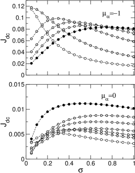
Figure 6: dc-current as a function of $\sigma$ for two different chemical potentials in a ring of $N=200$ sites with a two-band structure defined by $\epsilon_{o}=0,\;\epsilon_{e}=0.2$ and a reservoir with a constant density of states. Different plots correspond to $\Phi=0.05,0.1,0.2,0.3,0.4,0.5$ (upper panel) and $\Phi=0.2,0.3,0.4,0.5,0.6,0.7,0.8$ (lower panel).

The effect of ISP on the magnitude of the current through the gap is shown in the lower panel of Fig. 6. Within the weak coupling regime, the current is vanishingly small even for fields significantly larger than the energy gap ($\sim|\epsilon_{o}-\epsilon_{e}|$). This indicates that Zener tunneling alone (ie without dissipation) is not enough to generate a dc-response.

Figure 7: (Color online) dc-current as a function the chemical potential for a ring with $N=200$ sites and a two-band structure defined by $\epsilon_{o}=0,\;\epsilon_{e}=0.2$ and a reservoir with a constant density of states. The upper and lower panels correspond to weak ($\sigma=0.05$) and strong ($\sigma=0.85$) coupling regimes. Different plots correspond to different fields $\Phi=0.1,0.2,0.3,0.4,0.5,0.6,0.7,0.8$. The ones corresponding to the lowest and the highest fields are plotted in thick black and orange lines, respectively.

The behavior of $J_{dc}$ as a function of the chemical potential is shown in Fig 7. An important asymmetry is observed between the upper and lower bands, which is more pronounced for low fields. This is an indication of the relevance of the interband processes generated by the coupling of the electrons with the field. This discourages us from following the steps of the previous section in trying to make a parallel with a device based in two semi-infinite leads with the same band structure of the ring, since the latter would have two symmetric bands.

III.3 The ring with a random potential

This final subsection is devoted to analyze a disordered ring, with a random potential $\epsilon_{l}=\epsilon_{w}\gamma_{l}$, being $-1\leq\gamma_{l}\leq 1$, a random number.

Figure 8: Color online) dc-current as a function of the strength of ISP for a ring of $N=200$ sites with a random potential with amplitude $\epsilon_{w}=0.2$ and a reservoir with a constant density of states. Different panels correspond to different realizations of the random potential. Black circles, red squares, green diamonds and blue triangles correspond to $\Phi=0.2,0.3,0.4,0.5$, respectively.

The dc-current as a function of ISP strength for a fixed chemical potential is shown in Fig. 8 for four different realizations of the random potential. In all the cases a similar behavior is found: the current exhibits a wide and mild maximum at intermediate coupling and tend to zero in the limit of vanishing ISP. The magnitude of $J_{dc}$ at the maxima is smaller than in the two-band ring and significantly smaller than in the clean one-band system. As mentioned in the previous subsection the small current in the limit of weak coupling to the reservoir can be interpreted by noting that the formation of energy gaps in the structure of the energy levels of the chain tend to break the resonant behavior presented in the clean chain for small fields in the weak coupling regime. For small enough $\sigma$, the trend is $J_{dc}\propto\sigma$, as in the clean limit.

Figure 9: (Color online) dc-current as a function of the chemical potential for a ring of $N=200$ sites with a random potential with amplitude $\epsilon_{w}=0.2$ and a reservoir with a constant density of states. The upper and lower panels correspond to weak ($\sigma=0.05$) and strong ($\sigma=0.85$) coupling regimes. Different plots correspond to different fields $\Phi=0.1,0.2,0.3,0.4,0.5$. The ones corresponding to the lowest and the highest fields are plotted in thick black and violet lines, respectively.

As a function of the chemical potential, the dc-current displays fluctuations that become stronger in the strong coupling limit (see Fig. 9). The fluctuations bear a close resemblance with those observed in the behavior of the conductance of disordered quantum wires cf . A systematic analysis of the probability distribution of conductance $G$ defined in (27) over several disorder realizations as well as the behavior of $G$ as a function of the system length is left for the future.

IV Summary and conclusions

We have studied the transport properties of a dissipative tight-binding ring driven by means of a magnetic flux with a linear dependence in time. Dissipation is introduced by coupling the mesoscopic ring to an external macroscopic system that plays the role of a reservoir of particles and energy. We have extensively analyzed the behavior of the dc-component of the current along the ring as a function of the strength of dissipation and of the chemical potential of the reservoir for clean chains, chains with a two-band structure and an energy gap and disordered chains.

We have analyzed the influence of the specific model assumed for the reservoir and we conclude that this does not play any relevant role. In the weak coupling regime, the structure of the energy levels of the Hamiltonian describing the ring, seems to play a relevant role. Such structure determines the way in which contributions from different frequencies of the Green function couple through the pumping term in Eqs. (18), (19).

In all the cases we expect a vanishing dc-current in the Hamiltonian limit (vanishing ISP). For the case of the clean ring, we find that the current exhibits a maximum as a function of the ISP strength that seems to scale with $\Phi$. For small enough $\Phi$ this maximum can lye very close to the limit of vanishing ISP. The range of fields where a linear behavior of the dc-current as a function of $\Phi$ is observed depends on the strength of ISP. It is wide for strongly coupled systems and very narrow for weakly coupled ones. Remarkably, the behavior of the conductance of the system as a function of the chemical potential can be reproduced with a device consisting in a quantum dot with a constant density of states and two semi-infinite tight-binding chains with the same hopping parameter as the original one, attached to its left and right sides through a very large hopping element.

In the ring with a two-band structure, the behavior of the dc-current within each of the two conducting bands is similar to that observed in the one-band case. However, its magnitude is smaller and at fixed chemical potential and emf, the position of its maximum as a function of the ISP strength has a softer dependence with the emf. An important asymmetry is observed between the behavior of the current within the upper and lower bands, while inelastic scattering is essential to obtain a sizable magnitude of the current through the gap, irrespectively the intensity of the induced emf.

The disordered ring can be seen as the N-band extension of the two-band case. We have examined some typical realizations of the random potential and observed that as a function of inelastic scattering, the maximum in the dc-current takes place within the intermediate regime, becoming vanishingly small in the limit of weak coupling. As a function of the chemical potential, the current displays fluctuations following patterns that depend on the degree of inelastic scattering.

Our results are in agreement with the criteria based on symmetry arguments suggested for ratchet problems ser1 ; ser2 ; ser3 , according to which a dc-component of the current is possible provided that the equations of motion of the system are not invariant under symmetry operations that change the sign of the time-dependent current. In the case of the present problem the only possible symmetry that may introduce such an inversion, is time-reversal. This symmetry is an exact one in the pure Hamiltonian limit where the ring is isolated from the reservoir but it is immediately broken when the coupling to the reservoir is considered. Furthermore, we have found that the current grows linearly with the parameter that characterizes the strength of the inelastic scattering. This behavior has also been found in other pumped systems with broken time-reversal symmetry leh . The behavior of the dc-current in the case of the two-band and N-band (disordered) ring is also in agreement with the conclusions of Refs. lan1 ; lan2 ; gef1 ; gef2 ; brou which have been devoted to argue against the possibility of resistive behavior caused by Zener tunneling alone. In our case we were able to solve the problem exactly and to examine details of the behavior of the current for different strengths of inelastic scattering. For this reason, we think that our results provide a robust support to the idea that dissipation is an essential ingredient to obtain resistive behavior in this system.

V Acknowledgments

This work was in good part motivated by stimulating conversations with Sergej Flach, whom the author thanks very specially, as well as Yuval Gefen and Victor Gopar for useful correspondence and discussions. The author is grateful to Prof. Fulde for his kind hospitality at the MPIPKS-Dresden and to Drazen Zanchi and Leticia Cugliandolo for their hospitality at LPTHE, Paris, where this manuscript was finished. LA also thanks the support from the Alexander von Humboldt Stiftung, CONICET, Argentina and PICT 03-11609.

References

- (1) V. Chandrasekhar, R. A. Webb, M. J. Brady, M. B. Ketchen, W. J. Gallagher, and A. Kleinsasser, Phys. Rev. Lett. 67, 3578 (1991).
- (2) D. Mailly, C. Chapelier, and A. Benoit, Phys. Rev. Lett. 70, 2020 (1992).
- (3) R. Deblock, R. Bel, B. Reulet, H. Bouchiat, and D. Mailly, Phys. Rev. Lett. 89, 206803 (2002).
- (4) Y. Gefen, Y. Imry and Ya. Azbel, Phys. Rev. Lett. 52, 129 (1984).
- (5) Y. Imry, “Directions in Condensed Matter Physics”, edited by G. Grinstein, E. Mazenko (World Scientific, Singapore, 1986).
- (6) M. Büttiker, Y. Imry and R. Landauer, Phys. Lett. 96A, 365 (1983).
- (7) R. Landauer, IBM J. Res. Develop. 1, 233 (1957); R. Landauer, Phil. Mag. 21, 863 (1970).
- (8) M. Büttiker and R. Landauer, Phys. Rev. Lett. 54, 2049 (1985).
- (9) M. Büttiker, Phys. Rev. B 32, R1846 (1985).
- (10) D. Lenstra and W. van Haeringen, Phys. Rev. Lett. 57, 1623 (1986).
- (11) R. Landauer, Phys. Rev. B 33, 6497 (1986).
- (12) R. Landauer, Phys. Rev. Lett. 58, 2150 (1987).
- (13) Y. Gefen and D. J. Thouless, Phys. Rev. Lett. 59, 1752 (1987).
- (14) D. Lubin Y. Gefen and I. Goldhirsch, Phys. Rev. B 41, 4441 (1990).
- (15) G. Blatter and D. A. Browne, Phys. Rev. B 37, 3856 (1988).
- (16) P. Ao, Phys. Rev. B 41, 3998 (1990).
- (17) J. Avron and J. Nemirovsky, Phys. Rev. Lett. 68, 2212 (1992).
- (18) M. T. Liu, and C. S. Chu, Phys. Rev. B 61, 7645 (2000).
- (19) L. Arrachea, Phys. Rev. B 66, 045315 (2002).
- (20) S. Flach, O. Yevtushenko and Y. Zolotaruk, Phys. Rev. Lett. 84, 2358 (2000).
- (21) S. Denisov, S. Flach, A. A. Ovchinnikov, O. Yevtushenko, and Y. Zolotaryuk, Phys. Rev. E, 66, 041104 (2002).
- (22) S. Flach, Y. Zolotaryuk, A. E. Miroshnickenko and M. V. Fistul, Phys. Rev. Lett. 88, 184101 (2002).
- (23) J. Rammer and H. Smith, Rev. Mod. Phys. 58, 323 (1986).
- (24) A. P.Jauho, N. Wingreen and Y. Meir, Phys. Rev. B 50, 5528 (1994).
- (25) H. M. Pastawski, Phys. Rev. B 46, 4053 (1992).
- (26) J. Lehmann, S. Kohler, P. Hänggi, and A. Nitzan, J. Chem. Phys. 118, 3283 (2003).
- (27) J. Lehmann, S. Kohler, P. Hänggi, and A. Nitzan, Phys. Rev. Lett. 88, 228305 (2002).
- (28) M. Moskalets and M. Büttiker, Phys. Rev. B 68, 075303 (2003).
- (29) Y. Meir and N. S. Wingreen, Phys. Rev. Lett 68, 2512 (1992).
- (30) L. Arrachea, Eur. Phys. Jour. B 36, 253 (2003).
- (31) A. Levy Yeyati, Phys. Rev. B 45, 14189 (1992).