Coherent response of a low $T_{c}$ Josephson junction to an ultrafast laser pulse

Abstract

By irradiating with a single ultrafast laser pulse a superconducting electrode of a Josephson junction it is possible to drive the quasiparticles (qp’s) distribution strongly out of equilibrium. The behavior of the Josephson device can, thus, be modified on a fast time scale, shorter than the qp’s relaxation time. This could be very useful, in that it allows fast control of Josephson charge qubits and, in general, of all Josephson devices. If the energy released to the top layer contact $S1$ of the junction is of the order of $\sim\mu J$, the coherence is not degradated, because the perturbation is very fast. Within the framework of the quasiclassical Keldysh Green’s function theory, we find that the order parameter of $S1$ decreases. We study the perturbed dynamics of the junction, when the current bias is close to the critical current, by integrating numerically its classical equation of motion. The optical ultrafast pulse can produce switchings of the junction from the Josephson state to the voltage state. The switches can be controlled by tuning the laser light intensity and the pulse duration of the Josephson junction.

I Introduction

The characteristic frequency in the dynamics of a Josephson junction (JJ) is the so-called Josephson plasma frequency $\omega_{pJ}$ (e.g.$10\div 100GHz$). Coupling of a JJ to a microwave field leads to the well known lock-in conditions, which show up as Shapiro steps in the I/V characteristic. On the other hand, photo-response to radiation in a superconductor induces heat relaxation (bolometric effect barone ) and non equilibrium generation of quasiparticles (qp) testardi ; parker . Both phenomena are extensively studied since they are relevant for the fabrication of fast and sensitive detectors. The models used are phenomenological owen ; ivlev ; ser ; lindg ; semenov , mainly involving different temperatures associated to separate distributions of electrons and phonons out of equilibrium.

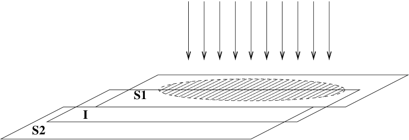
Figure 1: Sketch of the Josephson junction exposed to a laser radiation pulse.

Recently, laser light with pulses of femtosecond duration $\tau_{c}\in(10^{-14}s,10^{-13}s)$ has become available, as a source to test the photo-response of a JJ lindg . Ultrafast pulses can be extremely useful, in that they allow studying an unexplored regime in non equilibrium superconductivity. Indeed, photon absorption, by creating electron-hole (e-h) pairs at very high energies, drives the quasi-particle (qp) energy distribution out of equilibrium during the time $\tau_{c}$. The qp non-equilibrium distribution depends on the energy relaxation time parameter $\tau_{E}$, defined as the time by which a ‘hot’ electron is thermalized by repeated scatterings with other electrons or phonons. The process involves generation of many qp’s during energy degradation, until the system relaxes back to the equilibrium distribution function $n_{o}(\omega)$. This time scale is determined by the electron-electron interaction time $\tau_{e-e}$ and the electron-phonon interaction time $\tau_{e-ph}$, which are strongly material dependent kaplan , ranging from $4\cdot 10^{-7}s$ for $Al$ to $1.510^{-10}s$ for $Nb$. In this work we analyze the possibility that, keeping temperature quite low, ultrashort laser radiation induces direct switches out of the Josephson conduction state at zero voltage, due to coherent reduction of the critical current $J_{c}$.

There are many reasons for the switching from the zero to the resistive state in a Josephson junction. Among these, thermal escape thermal , quantum tunneling quantum , latching logic circuits latching and pulsed assisted escapepulse . A clear cut discrimination between different mechanisms can be difficult to achieve. In our case quantum escape is ruled out because the temperature is not expected to be low enough. Also, we assume that there is no external circuit to induce switching and re-set of the zero voltage state as in latching logic elements.

Pulsed assisted escape is a generic term for a large class of phenomena including in principle bolometric heating of the junction which is re-set in relatively slow times testardi . Production of quasiparticles generated by $X$-ray radiation has been studied up to recentlybarone2 ; ovchinnikov . A cascade follows, which increases the number of excitations and lowers their energy down to the typical phonon energy $\omega_{D}$ in a duration time, which is of the order of the nanoseconds. Subsequently, qp’s decay by heating the sample. However, the power of the laser can be reduced enough and both the substrate and the geometry can be chosen such that the energy released by the radiation on the junction can be small. On the other hand, appropriate experimental conditions can make the time interval between two pulses long enough, so that the bolometric response is negligible.

Generally speaking, junctions are more sensitive to pulses especially when their harmonic content is close to $\omega_{pJ}$, but this is not our case. In fact the laser carrier frequency ($\Omega\sim 100THz$) is quite high compared to $\omega_{pJ}$ and we consider the case $\Omega>>\tau_{c}^{-1}>\omega_{pJ}>\tau_{E}^{-1}$, what implies that little relaxation takes place during the duration of the pulse. $\tau_{c}$ should also be shorter than the pair-breaking time $\hbar/\Delta_{o}\sim 1\div 5ps$. Here $\Delta_{o}$ is the unperturbed gap parameter. Our approach assumes that, on a time scale intermediate between the pulse duration and the relaxation time $\sim\tau_{E}$, the order parameter of the irradiated superconductor is sensitive to the non-equilibrium qp distribution, which modulates it coherently till it switches out of the zero voltage state.

To analyze the dynamics of the order parameter and the way how the latter affects the Josephson current, we adopt a non-equilibrium formalism based on quasiclassical Green’s functions rammer ; belzig . The quasiclassical approach has been mostly used in the past in connection with the proximity effect belzig , as well as with non-equilibrium due to other space inhomogeneity conditionsamin . As far as we know, this is the first time that its extension to non-equilibrium in time is applied to a coherent response after an ultrafast laser irradiation.

The quasiclassical approximation to the Gorkov equations, is obtained by averaging over the period of the optical frequency $\Omega$, which is a fast time scalenoi . Our equations include the physics of the cascade process, which occurs when one focuses on the kinetics of the qp diffusion. A kinetic equation approach to the steady state non equilibrium qp distribution, including phonon scattering has been developed in ref.scalapino , for light irradiation, mostly in the microwave range. The cascade regime is extensively discussed in Ref.ovchinnikov , however it will not be specifically addressed here.

Instead, if the switching of the irradiated superconductor due to the ultrafast pulse takes place prior to the occurrence of qp relaxation, an approximate solution of the dynamical equations can be derived, which describes an istantaneous response of the order parameter.

We take a low $T_{c}$ JJ with an $s$-wave order parameter as the reference case (e.g. a high quality $Nb$ or $Al$ junction) and $T<<T_{c}$. The optical penetration depth of the laser light $\lambda_{\delta}$ in the topmost superconductor exposed to radiation $S1$ is assumed to be shorter than its thickness, so that any modification induced by the radiation field only involves $S1$ itself testardi (see. Fig.(1)). In a small size JJ the spatial variation of the order parameter along the lateral dimension of $S1$ is not taken into account, except when the qp diffusion process cannot be ignored.

We consider just one pulse of given duration $\tau_{c}$ which releases the energy ${\cal{E}}$ per pulse, by exciting $e-h$ pairs and by creating a non equilibrium distribution of qp’s. A related dimensionless quantity $q$, as defined in Eq. (7), parametrizes the strength of the perturbation due to the radiation. The perturbation is assumed to be small so that only the lowest order in the expansion in $q$ is retained. This allows us to derive a temporary reduction of the order parameter $\Delta$ induced by the pulse, as shown in Fig.(2). We do not give a detailed description for the relaxation of the non-thermal qp distribution in the irradiated superconductor. The self-energy terms corresponding to this process require further analysis. According to the Eliashberg formulation kaplan these terms affect the quasiparticle amplitude $Z(\omega)$ introducing changes in the phonon distribution and retardation in the response. Nevertheless, we expect that these self-energy terms become effective only on a longer time scale after the laser pulse. Our equations pinpoint a non retarded evolution of the order parameter prior to relaxation, which implies a reduction of the critical current. This shows that the coherent modulation of the gap parameter can produce switching of the junction out of the Josephson state.

The switches are studied numerically by solving the classical equation fo motion of a current biased JJ with current $J$ close to the critical curent $J_{c}$, during the excitation process. After the switching the dissipation in not treated selfconsistently: a standard dissipation, typical of thermal equilibrium, is assumed in the JJ dynamics, by adding a conductance term in the numerical simulation. We stress that the assumed model for dissipation determines the actual qp branch of the I-V characteristics, but does not affect substantially the switching probability. The switching from the Josephson state to the voltage state in the parameter space $(q,\tau_{c},J/J_{c})$ is reported in Fig.5. Interestingly, we find that for fixed value of $q$ and $J/J_{c}$ there is an optimum pulse duration to achieve the strongest sensitivity of the junction to the switching process. We show that this is due to the way how the non equilibrium qp’s distribution affects the pairing in $S1$. The paper is organized as follows.

In Section 2 we calculate the non equilibrium qp distributions immediately after the pulse, prior to relaxation.

In Section 3 we introduce the time dependent quasiclassical Keldysh Green functions formalism extended to the time domain, using the general frame given in appendix A. We calculate the correction to the single particle propagators to first order in $q$. A correction to the gap and to the Josephson critical current follows due to the laser pulse.

In Section 4 the dynamics of the JJ after the pulse is simulated numerically. Finally, a summary of our results is given in Section 5.

Appendix A collects the formulae of the quasiclassical approximation in the non equilibrium Keldysh theory, which are used in the core of the paper. In Appendix B we derive the kinetic equation for the non equilibrium distribution function which drives the relaxation of the system. The equations of motion for the quasiclassical retarded Green function is reported in appendix C, while the equation of motion for the advanced and Keldysh Green function can be derived in the same way .

II The non-equilibrium qp distribution

II.1 Non-equilibrium electron-hole pair excitations induced by optical irradiation

The optical frequencies ($\Omega\sim 100THz$) building the wavepacket of the laser pulse excite $e-h$ pairs at high energies. As explained in the introduction the non-equilibrium arising from the alteration of the qp distribution has a relaxation time $\tau_{E}$ which is long compared to the optical period: $\Omega\tau_{E}>>1$. In addition to this, the duration of the pulse $\tau_{c}\sim\omega_{c}^{-1}$ is even shorter than the pair breaking time, so that we expect that, in our case, dissipative phenomena do not affect the coherence of the superconductor on the time scale $\tau_{c}$.

Qp’s are generated as if the metal were normal, because superconductivity doesn’t play any role in their excitation at large energies. They propagate according to something very much like the free particle time-ordered Green’s function $g_{o}$ (from now on we put $\hbar=1$):

$$g_{o}^{T}(k;t-t^{\prime})\equiv-i\langle T[c_{k}(t)c_{k}^{\dagger}(t^{\prime})]\rangle=-ie^{-i\xi(t-t^{\prime})}\left[(1-n_{k})\theta(t-t^{\prime})-n_{k}\theta(-t+t^{\prime})\right]\>.$$ (1)

Here $\xi$ is the qp energy with momentum $k$ and is measured from the chemical potential $\mu$. $n_{k}$ is the qp distribution function. We assume that $e-h$ symmetry is conserved in the excitation process, so that $\mu$ is not altered with respect to its equilibrium value.

The equation of motion for the Green’s function $\tilde{g}$ in the presence of the radiation field is:

$$\left(i\frac{\partial}{\partial t}-\frac{1}{2m}[\vec{\nabla}_{r}-\frac{e}{c}\vec{A}(\vec{r},\vec{R},t)]^{2}+\mu\right)\>\tilde{g}(\vec{r},\vec{R},t,t^{\prime})=\delta(r)\delta(t-t^{\prime})\;,$$ (2)

$\vec{r}$ is the relative space coordinate, while $\vec{R}$ is the center of mass coordinate. The vector potential is a wave-packet centered at frequency $\Omega$ according to:

$$\vec{A}(\vec{r},\vec{R},t)=\sum_{\pm}\sum_{\vec{p}}\vec{a}_{\pm}(\vec{p},\vec{R},t)e^{\mp i(\vec{p}\cdot\vec{r}-\Omega t)}\;.$$ (3)

Here $\vec{a}_{\pm}$ are slowly varying ’envelope’ functions of $\vec{R}$ on the size of the irradiated spot and on the time scale $\Omega^{-1}$. We look for solutions of eq.(2) in the form:

$$\tilde{g}(\vec{r},\vec{R};t,t^{\prime})=g(\vec{r},\vec{R};t,t^{\prime})+\sum_{\pm}\sum_{\vec{p}}g^{\pm}(\vec{p},\vec{R},t,t^{\prime})e^{\mp i(\vec{p}\cdot\vec{r}-\Omega t)}\;\;,$$ (4)

where $g$ and $g^{\pm}$ are slowly varying functions of $\vec{R}$ and $t$ on the same scales. A similar expansion can be done w.r.to the variable $t^{\prime}$. Following Eq. (4), a decomposition of eq.(2) into harmonics arisesnoi . We define the zero order harmonic equation as the one that does not contain exponentials $e^{\pm i\Omega t}$. By averaging over a period $\Omega^{-1}$ we neglect harmonics of order two, or higher. This amounts to include one photon excitation processes only, with released energy ${\cal{E}}$. Some extra details can be found in Appendix A:

$$\left(i\frac{\partial}{\partial t}+\frac{1}{2m}\nabla^{2}_{r}+\frac{e^{2}}{mc^{2}}\sum_{\vec{p}^{\prime},\vec{p}^{\prime\prime}}\vec{a}_{+}(\vec{p}^{\prime},\vec{R},t)\vec{a}_{-}(\vec{p}^{\prime\prime},\vec{R},t)e^{i(\vec{p}^{\prime}-\vec{p}^{\prime\prime})\cdot\vec{r}}\>+\mu\right)g(\vec{r},\vec{R},t,t^{\prime})=\delta(r)\delta(t-t^{\prime})\;.$$

Fourier transforming w.r.to $\vec{r}$ ( $\vec{r}\to\vec{p}\to\xi$) we have:

$$\left(i\frac{\partial}{\partial t}-\left(\frac{p^{2}}{2m}-\mu\right)\right)g(\vec{p},\vec{R},t,t^{\prime})+\frac{e^{2}}{mc^{2}}\sum_{\vec{p}^{\prime},\vec{p}^{\prime\prime}}\vec{a}_{+}(\vec{p}^{\prime},\vec{R},t)\vec{a}_{-}(\vec{p}^{\prime\prime},\vec{R},t)\>g(\vec{p}^{\prime}-\vec{p}^{\prime\prime}-\vec{p},\vec{R},t,t^{\prime})=\delta(t-t^{\prime})\;.$$ (5)

The radiation field generates and annihilates high energy $e-h$ pairs. Hence we assume that the forcing term conserves the total impulse, $\vec{p}^{\prime}+\vec{p}^{\prime\prime}\sim 0$, but $\vec{p}^{\prime}-\vec{p}^{\prime\prime}$ transfers an energy $2\xi$ to the electrons. Therefore we take the coupling term in the Hamiltonian as:

$$\frac{e^{2}}{mc^{2}}\vec{a}_{+}(\vec{p}^{\prime},\vec{R},t)\vec{a}_{-}(\vec{p}^{\prime\prime},\vec{R},t)\to q\>\frac{\omega_{c}}{\sqrt{\pi}}e^{-\frac{1}{2}\omega_{c}^{2}t^{2}}\>\delta(2\xi+\xi^{\prime})\>\delta(\vec{p}^{\prime}+\vec{p}^{\prime\prime})\>.$$ (6)

A Gaussian shaped time dependence has been chosen for the pulse with half-width $\omega_{c}^{-1}$, while the space dependence has been neglected for simplicity. In Eq. (6) the dimensionless quantity appears:

$$q\sim\frac{e^{2}}{c}\>\frac{\omega_{D}}{\Omega}\>\;\frac{{\cal{E}}}{m\Omega^{2}R^{2}_{o}}\>,$$ (7)

Where $R_{o}$ is the laser spot (see Eq.16). Here the number of excited $e-h$ pairs is $\sim\Omega/\omega_{D}$, with $\omega_{D}$ the Debye energy. Experiments testardi ; lindg show that the energy released by the pulse can be very low, so that we will always expand in $q$. In fact, while in the case of an $rf$ radiation $q\sim 1$, in the case of a femtosecond laser pulse $q\sim 0.01\div 0.1$, corresponding to a fraction of $\mu J$ released per pulse on the superconducting surface of $\sim 100\mu m^{2}$.

The zero order harmonic equation, Eq. (5), becomes :

$$\left(i\partial_{t}-\xi\right)g(\xi;t,t^{\prime})+q\frac{\omega_{c}}{\sqrt{\pi}}e^{-\frac{1}{2}\omega_{c}^{2}t^{2}}g(-\xi;t,t^{\prime})=\delta(t-t^{\prime}))\;.$$ (8)

To derive the non-equilibrium correction to the qp distribution function, the kinetic equation 58 should be solved. In place of this we proceed in this work in an heuristic way. Our approach lacks mathematical rigour, but singles out directly the role of the laser induced $e-h$ excitations at frequencies $(\Omega-\omega_{c},\Omega+\omega_{c})$. Our result is valid in the limit of large $\xi$’s and zero temperature, before relaxation takes place.

We solve Eq(8) for the retarded Green’s function for $t>0$ and $-t^{\prime}\sim 0^{+}$ by truncating the Dyson equation to lowest order in $q$:

$$g^{R}(\xi;t,t^{\prime})=g_{o}^{R}(\xi;t-t^{\prime})-q\frac{\omega_{c}}{\sqrt{\pi}}\int dt^{\prime\prime}g_{o}^{R}(\xi;t,t^{\prime\prime})e^{-\frac{1}{2}\omega_{c}^{2}{t^{\prime\prime}}^{2}}g_{o}^{R}(-\xi;t^{\prime\prime}-t^{\prime})$$

$$=g_{o}^{R}(\xi;t-t^{\prime})+iq\frac{\omega_{c}}{\sqrt{\pi}}\int_{-\infty}^{+\infty}\frac{d\omega}{2\pi}\frac{e^{-i\omega t}}{\omega-\xi+i0^{+}}\int_{0^{+}}^{+\infty}dt\>e^{i(\omega-\xi)t}e^{-\frac{1}{2}\omega_{c}^{2}t^{2}}\;,$$ (9)

where $g_{o}^{R}(\omega)=\{\omega-\xi+i0^{+}\}^{-1}$ is the Fourier transform of the retarded Green’s function. The time integral can be expressed in terms of the function $w[z]\equiv e^{-z^{2}}\>erfc\>(-iz)$. If we now approximate Eq. (9) by evaluating $w[z]$ only at the pole and use the the integral representation of the step function:

$$\theta(t)=\frac{e^{izt}}{2\pi i}\int_{-\infty}^{+\infty}d\omega\frac{e^{-i\omega t}}{\omega-z}\;\;\;for\;\;\Im mz<0\>\>\>,$$ (10)

the correction $\delta g^{R}(\xi,t)$ to $g^{R}$ for $\xi>>0$, which includes the non equilibrium qp ’s distribution, is:

$$\delta g^{R}(\xi,t,0^{-})=-\frac{q}{\sqrt{2}}e^{-i(\xi-i0^{+})t}\>\>w\left[-2\xi/(\sqrt{2}\omega_{c})\right]\>\>\theta(t),$$ (11)

From eq.(11) we obtain the time ordered Green’s function for $t>0,\>t^{\prime}=0^{-}$ and $\xi>0$:

$$g(\xi,t>0,0^{-})=(-i)e^{-i(\xi-i0^{+})t}\>\theta(t)\>\left(1-\frac{q}{\sqrt{2}}\>\>\rho\left[2\xi/(\sqrt{2}\omega_{c})\right]\right),$$ (12)

with

$$\rho[x]\equiv e^{-x^{2}}\frac{2}{\sqrt{\pi}}\int_{0}^{x}ds\>e^{s^{2}}\>\>.$$ (13)

$\rho[x]$ increases linearly with $x$ and it decreases slowly, as $1/x$, at large arguments. In Eq. (12) we have neglected $\Re e[w]$ because $|\xi|>>0$.

Eq. (12) is to be compared with the free propagating time ordered Green’s function of eq.(1) for the same time arguments. Comparison yields the amount by which the distribution function is driven out of the equilibrium:

$$\delta n(\xi)\approx\frac{q}{\sqrt{2}}\>\rho\left[2\xi/(\sqrt{2}\omega_{c})\right]\;\;\;for\;\;|\xi|>>\Delta_{o}\>\>\>.$$ (14)

Note that the expression of Eq. (14) changes sign according to $sign\;\{\xi\}$. This stems from the assumed $e-h$ symmetry. In turn this implies that no charge imbalance occurs.

Eq. (14) can be considered as the non equilibrium distribution for qp ’s starting at the time of the pulse $t\sim 0^{+}$.

In the absence of relaxation, a change in the available qp density of states follows. Because $(g^{R}(\xi,\omega))^{*}=g^{A}(\xi,\omega)$ if $\omega$ is real, the correction to the density of state $\delta\nu(\xi)$ is:

$$\delta\nu(\xi)=-\frac{1}{\pi}\left(\delta g^{R}-\delta g^{A}\right)(\xi,0^{+})\approx\frac{q}{\pi\sqrt{2}}\>\rho\left[2\xi/(\sqrt{2}\omega_{c})\right]\;\;\;for\;\;\xi>0\>\>\>.$$ (15)

The first stages of the relaxation process involve the inelastic diffusion of qp’s in the medium which is qualitatively discussed in the next section.

II.2 Inelastic diffusion of the qp’s at initial times

Let us discuss shortly what was neglected in the derivation of the change in the equilibrium qp distribution $\delta n(\xi)$ given by Eq.(14).

The single particle Green’s function $g(p,R,t,t^{\prime})$ is assumed to be a slowly varying function of $(t+t^{\prime})/2=\overline{t}$ and a fast varying function of $t-t^{\prime}$. Fourier transforming w.r.to the latter variable ( see Appendix A ) there is an $\omega$ dependence even in the stationary case ( i.e. with no $\overline{t}$ dependence). This $\omega$ dependence is determined by the frequency dependent Eliashberg $e-ph$ coupling $\alpha^{2}F(\omega)$ and is contained in the $e-ph$ self-energy $M_{e-ph}(\omega)$ grimvall . Accordingly, the complex qp renormalization parameter $Z_{n}(\omega)$ is defined by $[1-Z_{n}(\omega)]\omega=M_{e-ph}(\omega)$. In our derivation we have not included the self-energy, so that we are implicitly taking $Z_{n}(\omega)\to 1$, what applies for large $\omega(\sim\Omega)$, prior to relaxation.

Moreover, because the system is in the superconducting state, we should have dealt with the corresponding superconducting parameter $Z_{s}(\omega)$. The latter is derived together with the complex gap parameter $\Delta(\omega,\overline{t})$ with $\Delta(\Delta_{o},\overline{t}=0^{-})=\Delta_{o}$ from the coupled Eliashberg equations ( we drop the overline on $t$ in the following ).

The procedure of averaging over the fast time scale $\Omega^{-1}$ singles out two frequency components of $\Delta(\omega,t)$ and $Z_{s}(\omega,t)$: $\omega=\Delta_{o}$ and $\omega=\Omega$ as a consequence retardation arises from frequencies up to $10\omega_{D}$ is neglected. $\Omega$ is so large that $Z_{s}$ and $Z_{n}$ do not differ sizeably. In fact, their real parts differ by a quantity of the order of $(\omega_{D}\Delta_{o}/\Omega^{2})^{2}\ln(\omega_{D}/\Delta_{o})$. $\Delta(\Omega,t)$ itself is expected to be so small that it can be neglected alltogether. Indeed, in connection with eq. 48 of Appendix A we do not discuss the self-energy terms. Of course this approximation breaks down on the time scale of $e-ph$ relaxation.

Let us now discuss the $t$ dependence. The equation of motion for the qp distribution function $n(\vec{R},t)$ is derived in Appendix B, where we take $n_{T}=0$, because we neglect charge imbalance corrections.

In averaging over a few optical periods the kinetic equation for $\delta n_{L}$, the electric field $\vec{E}$ averages to zero. The qp relaxation is governed by the collision integral $I[n(\vec{R},t);t]$ which describes the inelastic processes. In Ref.ovchinnikov the cascade of the $e-h$ excitations due to inelastic scattering is studied in detail. Two stages occur. In the first stage e-e interactions multiply the number of excited qp’s in the energy range from $\Omega$ to $\omega_{D}$ which is taken as the cutoff energy of the pairing interaction. This happens in a time interval short w.r.to the pulse duration ($\sim 10^{-14}s$). In the second stage a much slower relaxation process takes place, by which the energy of the qp’s reaches $\Delta$. This process involves electron-phonon scattering on a time scale $\hbar\omega_{D}^{2}/\Delta^{3}\sim 10^{2}ns$ which is much larger than any time scale in our problem. Here we will leave this stage aside. In the time interval we are concerned with, we have little relaxation and the energies involved are $\omega>>\Delta$.

According to Eq. (56) the distribution function prior to relaxation deviates from the equilibrium value by the quantity $\delta n_{L}=-2\delta n(\xi)$ given by Eq. (14). There is no explicit dependence on $\omega$ in our correction, becauise retardation is nelgected. Still qp’s diffuse in space inside the junction over a characteristic distance $R_{o}\sim\sqrt{D\tau_{e-e}}$, where $D$ is the diffusion coefficient. Hence

$$\delta n_{L}(\xi,\vec{R},t)=-2\frac{R_{o}^{2}}{R_{o}^{2}+Dt}\>\delta n(\xi)\>e^{\left\{-\frac{R^{2}}{R_{o}^{2}+\frac{D}{t}}\right\}}\>\>\>.$$ (16)

For relatively large times $\tau_{e-ph}>>t>>R_{o}^{2}/D$ we will ignore the spatial dependence by putting $R=0$. This is the first step of a perturbative analysis of the non equilibrium distribution functions.

III Changes of the superconductive properties on the time scale $\omega_{c}^{-1}$

III.1 The correction to the gap parameter

In this Subsection we derive the Keldysh Green’s function in the presence both of a time dependent gap $\Delta(t)$ and of a non-equilibrium qp distribution as given by Eq. (16). We assume weak coupling superconductivity and we neglect here the frequency dependence of the $e-ph$ coupling parameter $\lambda$. This follows from the neglecting the retardation effects mentioned in Sec. IIb on time scales much faster than the $e-ph$ relaxation time. From the Keldysh Green’s function $\hat{g}^{K}$ (where the hat denotes matrix representation in the Nambu space, see appendix A) we recalculate the gap self-consistently, according to the formula:

$$\Delta(t)=-\frac{\nu(0)\lambda}{4}\int_{-\infty}^{\infty}<f^{K}({\vec{p}/|\vec{p}|},\omega,t)>_{\vec{v}_{F}}\;d\omega\;.$$ (17)

The average over the direction of the momenta on the Fermi surface is indicated. The Keldysh Green’s function in thermal equilibrium is:

$$\hat{g}_{o}^{K}=\tanh\frac{\beta\omega}{2}\left(\hat{g}^{R}-\hat{g}^{A}\right)\>.$$ (18)

Out of equilibrium we use the definition:

$$\hat{g}^{K}=\hat{g}^{R}\hat{h}-\hat{h}\hat{g}^{A}\>\>.$$ (19)

However, $\hat{h}$ defined in appendix B is here diagonal, because we assume that no charge imbalance arises. Hence, up to first order in $q$,

$$\delta\hat{g}^{K}\approx n^{0}_{L}(\hat{g}^{R}_{ad}-\hat{g}^{A}_{ad})+\delta n_{L}(\hat{g}_{o}^{R}-\hat{g}_{o}^{A})\>.$$ (20)

Here $n_{L}^{o}=\tanh(\beta\omega/2)$ is the equilibrium distribution and $\hat{g}^{R}_{ad}-\hat{g}^{A}_{ad}$ is introduced in Appendix C (see Eq.60) and is discussed in the following.

We now first derive the contribution coming from the second term of Eq. (20). We start from the outset using Eq. (16) and performing the quasiclassical approximation. The latter involves an energy integration:

$$\delta n_{L}\cdot\left(\hat{g}_{o}^{R}-\hat{g}_{o}^{A}\right)\equiv\frac{i}{\pi}\int_{-\infty}^{+\infty}d\;\xi\>\delta n_{L}(\xi,t)\cdot\left(\hat{g}_{o}^{R}(\xi,\omega,t)-\hat{g}_{o}^{A}(\xi,\omega,t)\right)\>.$$ (21)

Using the equilibrium BCS functional forms, the Green’s functions appearing on the diagonal of $\hat{g}^{A/R}$ are gork :

$$g^{R}(\xi,\omega)=\frac{u^{2}_{\xi}}{\omega-E_{\xi}+i0^{+}}+\frac{v^{2}_{\xi}}{\omega+E_{\xi}+i0^{+}}\>,$$ (22)

$$g^{A}(\xi,\omega)=\frac{u^{2}_{\xi}}{\omega-E_{\xi}-i0^{+}}+\frac{v^{2}_{\xi}}{\omega+E_{\xi}-i0^{+}}\>.$$ (23)

The equilibrium values for $u_{\xi}$ and $v_{\xi}$ are:

$$u_{\xi}^{0}=\left(\frac{1}{2}(1+\frac{\xi}{E})\right)^{\frac{1}{2}}\>,\hskip 28.45274ptv_{\xi}^{0}=\left(\frac{1}{2}(1-\frac{\xi}{E})\right)^{\frac{1}{2}}\>,$$ (24)

with $E=\sqrt{{\xi}^{2}+|\Delta_{o}|^{2}}$. From now on we will drop the subscript in the equilibrium gap parameter (i.e. $\Delta\equiv\Delta_{o}$ if no time dependence is indicated explicitely). Because the factor $\delta n_{L}(\xi,t)$ appearing in eq.(21), as given by Eq. (16) is odd w.r. to $\xi$ only the second term in $u^{2}$ and $v^{2}$ survives, when the integral in Eq. (21) is performed. Let us consider the case $\omega>\Delta$ only and specialize Eq. (21) to its diagonal part. According to Eq. (16) we have:

$$\Re e\left\{\delta n_{L}\cdot g^{R}_{o}\right\}=\Re e\left\{-\frac{\sqrt{2}i}{\pi}\>q(t)\>\int_{-\infty}^{+\infty}d\>\xi\frac{\xi}{2E}\>\rho\left[2\xi/(\sqrt{2}\omega_{c})\right]\left(\frac{1}{\omega-E+i0^{+}}-\frac{1}{\omega+E+i0^{+}}\right)\right\}=$$

$$=-q(t)\>2\sqrt{2}\>\rho\left[2(\omega^{2}-|\Delta|^{2})^{\frac{1}{2}}/(\sqrt{2}\omega_{c})\right]\>.$$ (25)

Here we have defined the function $q(t)$:

$$q(t)=q\>\>\frac{\pi R_{o}^{2}}{R_{o}^{2}+Dt}\>.$$ (26)

Doing similarly for $g^{A}$ and subtracting, the imaginary part cancels:

$$\delta n_{L}\cdot\left({g}_{o}^{R}-{g}_{o}^{A}\right)=-q(t)4\sqrt{2}\>\rho\left[2(\omega^{2}-|\Delta|^{2})^{\frac{1}{2}}/(\sqrt{2}\omega_{c})\right]\;,\;\;for\;\;\omega>\Delta\>\>\>.$$ (27)

Here the largest contribution of the non-equilibrium excitations arises from $\omega\sim\omega_{c}$. On the other hand $\omega_{c}$ can be larger or smaller than $\omega_{D}$.

Now we evaluate the correction due to $\hat{g}^{R}_{ad}-\hat{g}^{A}_{ad}$. In appendix C we show that an adiabatic solution of the motion equation of $g^{R,A}$ is possible, in the sense that the functional dependence on $\omega$ is the same as the equilibrium one, but the gap parameter changes slowly with time (see Eq. (60)):

$$\hat{g}_{ad}^{R(A)}=+(-)\frac{\hat{M}}{\sqrt{(\omega\pm i0^{+})^{2}-|\Delta(t)|^{2}}}\>$$ (28)

with

$$\hat{M}=\left(\begin{array}[]{cc}\omega&\Delta(t)\\ -\Delta(t)^{*}&-\omega\end{array}\right).$$ (29)

This functional form for the $R/A$ functions is obtained if the $e-h$ symmetry is maintained and if one neglects the diffusion in space-time which will be mainly important at intermediate times ovchinnikov .
This adiabatic approximation in the advanced and retarded Green’s functions allows us to write the Keldysh propagator in the form:

$$g^{K}=g_{ad}^{K}-q(t)4\sqrt{2}\>\rho\left[2(\omega^{2}-|\Delta|^{2})^{\frac{1}{2}}/(\sqrt{2}\omega_{c})\right]\>.$$ (30)

To calculate $f^{K}$ we resort to the analogous of eq.(59) which is valid for $\hat{g}^{K}$: $f^{K}=g^{K}\Delta/\omega$. Hence we have:

$$f^{K}=f_{ad}^{K}-q(t)4\sqrt{2}\>\frac{\Delta}{\omega}\>\rho\left[2(\omega^{2}-|\Delta|^{2})^{\frac{1}{2}}/(\sqrt{2}\omega_{c})\right]\;\;\;for\;\;\omega>>\Delta\>\>\>.$$ (31)

Now we insert Eq. (31) into Eq. (17) and consider the linear correction to the gap of the irradiated contact according to :

$$\Delta(t)=\Delta+\delta\Delta(t)\>.$$

Here $\delta\Delta(t)$ is the correction to the unperturbed gap parameter $\Delta$ due to the radiation. In the limit of zero temperature, up to first order in $q(t)$ and $\Delta/\omega_{D}$, $\delta\Delta(t)$ is given by:

$$\frac{\delta\Delta(t)}{\Delta}=-\frac{q(t)4\sqrt{2}}{ln(2\omega_{D}/\Delta)-2+{\cal{O}}(\Delta^{2}/\omega_{D}^{2})}\int_{\Delta}^{\omega_{D}}\;\frac{d\omega}{\omega}\>\rho\left[2(\omega^{2}-|\Delta|^{2})^{\frac{1}{2}}/(\sqrt{2}\omega_{c})\right]\>.$$ (32)

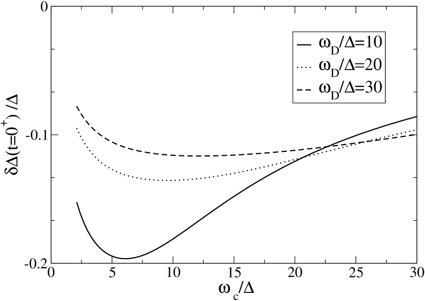
Figure 2: Variation of the gap immediately after the pulse vs the inverse of duration of the pulse $\tau_{c}^{-1}=\omega_{c}$ in units of $\Delta$. Our approximations break down for very low ratios $\omega_{c}/\Delta$ (long pulses). On the other hand, large $\omega_{c}/\Delta$ represent very short pulses: this situation is unrealistic with the available optical devices.

It is interesting to note that the correction arising from the adiabatic dynamics has the role of renormalizing the coupling $q(t)$ via the prefactor $-[ln(2\omega_{D}/\Delta)-2]^{-1}$. This prefactor is negative because $ln(2\omega_{D}/\Delta)>2$. Therefore Eq. (32) shows that the gap of the irradiated superconductor is decreased due to the non equilibrium distribution of the qp excitations.

Eq. (32) has the same structure as Eq. (14) of ref.scalapino . There is a striking difference however. The inverse square root singularity at the gap threshold, which shows up in Eq.(14) of ref.scalapino does not appear in Eq. (32).

The inverse square root singularity originates from the unperturbed density of states at the excitation threshold and is usually present in non-stationary superconductivity eliashberg . It is responsible for retardation and oscillating tails. In our case, the gap threshold plays a little role, because we do not have extensive pair-breaking and q.p. generation at energies $\sim\Delta$. Hence, just a tail $\sim 1/\omega$ survives in the integrand.

In Fig.(2) the variation of the gap immediately after the pulse ($t\sim 0$), is plotted vs the inverse of the pulse duration $\omega_{c}$ in units of $\Delta$, for different values of $\omega_{D}$. Our approximations are not valid when the pulse becomes too long (very low values of $\omega_{c}/\Delta$). For longer pulses the integrand in Eq. (32) has a narrow peak lined up at the gap threshold. In this case the inverse square root singularity in the density of states at the gap threshold is important and the adiabatic approximation Eq.(30) breaks down.

For shorter pulses the peak becomes broader and is centered at larger $\omega$’s. If the integration range is small, the result is quite sensitive to the location of the peak (see full line in Fig. (2)): most remarkably, a minimum appears in the curve when the pulse is rather long ($\omega_{c}/\omega_{D}<5$). By contrast, the gap correction is rather flat w.r.to changes of $\omega_{c}$ when $\omega_{D}/\Delta$ is larger (broken and dotted line in Fig.2).

III.2 Correction to the Josephson current

In this subsection we derive the correction to the Josephson current arising from the two terms of the anomalous propagator $f(R,t,t^{\prime})$ given by Eq. (31). Eq.s(30,31) show that the non equilibrium Keldysh Green functions of the irradiated superconductor can be separated into two terms. The first one is what we call the ’adiabatic’ contribution, while the second one is strongly dependent on the non equilibrium qp’s distribution function and is first order in $q(t)$.
Within the linear response theory in the tunneling matrix element $|T_{o}|^{2}$, the pair current at zero voltage is:

$$J(\vec{R}=0,t)=2e|T_{o}|^{2}\int_{-\infty}^{\infty}\;dt^{\prime}e^{2ieV(t-t^{\prime})}$$

$$\left({f^{>}}_{1}^{\dagger}(0,t,t^{\prime})\>f^{A}_{2}(0,t^{\prime},t)+{f^{R}}^{\dagger}_{2}(0,t,t^{\prime})\>f^{<}_{1}(0,t^{\prime},t)\right)\;,$$ (33)

where $|T_{o}|^{2}$ is assumed to be independent of energy, for simplicity. The current of Eq. (33)is evaluated at the junction site, defined by $\vec{R}=0$ and the irradiated superconducting layer $S1$ is labeled by 1 here, while the superconductor unexposed to radiation $S2$ is labeled by 2. The perturbed Josephson current has an adiabatic term $J^{ad}(t)$ obtained by inserting the first term of Eq. (31) into Eq. (33), plus a correction $\delta J(t)$ arising from the second term of Eq. (31). Using the definitions ${f}^{K}={f}^{>}+{f}^{<}$ and ${f}^{R}-{f}^{A}={f}^{>}-{f}^{<}$ and expanding to lowest order in $q(t)$ the adiabatic critical current is:

$$J^{ad}=J^{ad}_{c}(t)\sin(\varphi),\;\;\;\;\;\;J^{ad}_{c}(t)=\frac{\pi\hbar\Delta}{2eR_{N}}\left(1+\frac{\delta\Delta(t)}{2\Delta}\right)\>,$$ (34)

where $R_{N}$ is the normal resistence, $\Delta$ is the unperturbed gap parameter of both contacts (assuming $\Delta_{1}=\Delta e^{i\varphi}$ and $\Delta_{2}=\Delta$ in the absence of laser perturbation), and $\delta\Delta(t)/\Delta$ is given by Eq. (32). Denoting by $\delta f^{K}$ the second term of Eq. (31) the correction $\delta J(t)$ is:

$$\delta J(t)=e|T_{o}|^{2}\int_{-\infty}^{\infty}\;d\omega\>\left((\delta{f}^{K}(\omega+ieV))^{\dagger}_{1}{f}^{A}_{2}(\omega-ieV)+({{f}}^{R}(\omega+ieV))^{\dagger}_{2}(\delta{f}^{K}(\omega-ieV))_{1}\right)\>.$$ (35)

At zero temperature and $V=0$, this gives:

$$\delta J(t)=\frac{\pi\hbar}{eR_{N}}\int_{-\infty}^{\infty}\;d\omega\>\frac{|\Delta|^{2}q(t)}{\omega}\rho\left[2(\omega^{2}-|\Delta|^{2})^{\frac{1}{2}}/(\sqrt{2}\omega_{c})\right]$$

$$\left(\frac{e^{-i\varphi}}{\sqrt{(\omega+i0^{+})^{2}-|\Delta|^{2}}}+\frac{e^{i\varphi}}{\sqrt{(\omega-i0^{+})^{2}-|\Delta|^{2}}}\right)\>.$$ (36)

which is zero for parity. This conclusion holds because we assume that no charge imbalance occurs. If $V\neq 0$ the contributions to the integral evaluated in the complex plane are finite.
$\delta J(t)$ is a $cos\varphi$-like correction. In the unperturbed Josephson effect a ’$cos\varphi$’ term only arises when $V>2\Delta$ barone . By contrast, our calculation shows that a $cos\varphi$ term can arise in the Josephson current with a small nonzero voltage in the presence of an ultrafast laser pulse.

IV Classical dynamics of the irradiated junction

In this section we integrate the classical equation of motion of the irradiated junction numerically. Here we discuss the possibility that the laser pulse induces switches of the junction from the zero voltage state, to the resistive state. The characteristics of the Josephson junction for a finite voltage, is obtained within the RCSJ (resistively and capacitively shunted junction) model barone . The phase of the superconductor S2 is taken as the reference phase.

In the absence of the pulse, the junction is biased by a current constant in time $J_{b}$. As discussed in the previous Section, the pulse activates the superconductor S1 by varying its gap dynamically in time.

Consequently, a voltage $V$ arises at the junction, related to the dynamics of the phase difference $\varphi(t)$. The latter solves the differential equation:

$$\ddot{\varphi}+Q_{0}^{-1}\dot{\varphi}+\frac{J_{c}^{ad}(t)}{J_{c}^{o}}\sin\varphi(t)=\gamma\;,$$ (37)

where $\gamma={J_{b}/J_{c}^{o}}$ and $J_{c}^{o}={(\pi\hbar\Delta)/(2eR_{N})}$ is Josephson critical current of the unperturbed junction. The time-dependent driving term is deduced from Eq. (34). We assume $\omega_{pJ0}>\tau_{E}^{-1}$ ($\tau_{E}^{-1}(Nb)\sim 7GHz$), where $\omega_{pJ0}$ is the plasma frequency at zero bias. This condition is satisfied for high quality $Nb$ junctions, where $\omega_{pJ0}$ is in the range $40GHz\div 120GHz$ wallraff , but it holds also if we take into account the dependence of the plasma frequency on $\gamma$: $\omega_{pJ}=\omega_{pJ0}(1-\gamma^{2})^{(1/4)}$. At $\gamma=0.98$ the term $(1-\gamma^{2})^{(1/4)}=0.44$: this still gives a large plasma frequency for the given range. In any case the plasma frequency changes marginally when the energy is degradated into heat if $q$ is small. Under this conditions the relaxation process occurs long after the switch to resistive state.

In Eq. (37), $Q_{0}=\omega_{pJ0}R(\varphi)C$ is the quality factor, where $R(\varphi)$ is the junction intrinsic resistance, which is in general a non-linear function of the phase. The dissipative $Q^{-1}_{0}\dot{\varphi}$ term includes thermal incoherent pair breaking effects at equilibrium. In the simulation we use both a constant junction resistance $R$ and a patchwork model given by Likharev :

$$Q^{-1}(\dot{\varphi})=Q_{0}^{-1}\frac{\omega_{pJ}}{\Delta}\frac{(\frac{\dot{\varphi}\omega_{pJ}}{\Delta})^{N}}{1+(\frac{\dot{\varphi}\omega_{pJ}}{\Delta})^{N}}$$ (38)

with $N=16$ and $Q_{0}^{-1}=0.636$, which corresponds to a normal resistance above the gap $R_{N}=(\omega_{pJ}\varphi_{0})/(cJ^{0}_{c})$. In general we ignore the direct dependence of $R(\varphi)$ on the phase. By the way, $Q$ should also depend on the energy which is released by each single laser pulse due to the incoherent pair breaking process. However, under the hypothesis that this energy is very low we assume that the quality factor, due to the optically induced normal resistance of the sample, is constant within the considered energy range.
Actually, in the presence of the pulse, also the current contribution of Eq. (35) should be plugged into the l.h.s. of Eq. (37). This current term depends on the voltage $V=\dot{\varphi}$. However, in view of the fact that in this work we are only concerned with the switching of the junction out of the zero voltage state, we do not derive the full dynamics of the phase self-consistently.

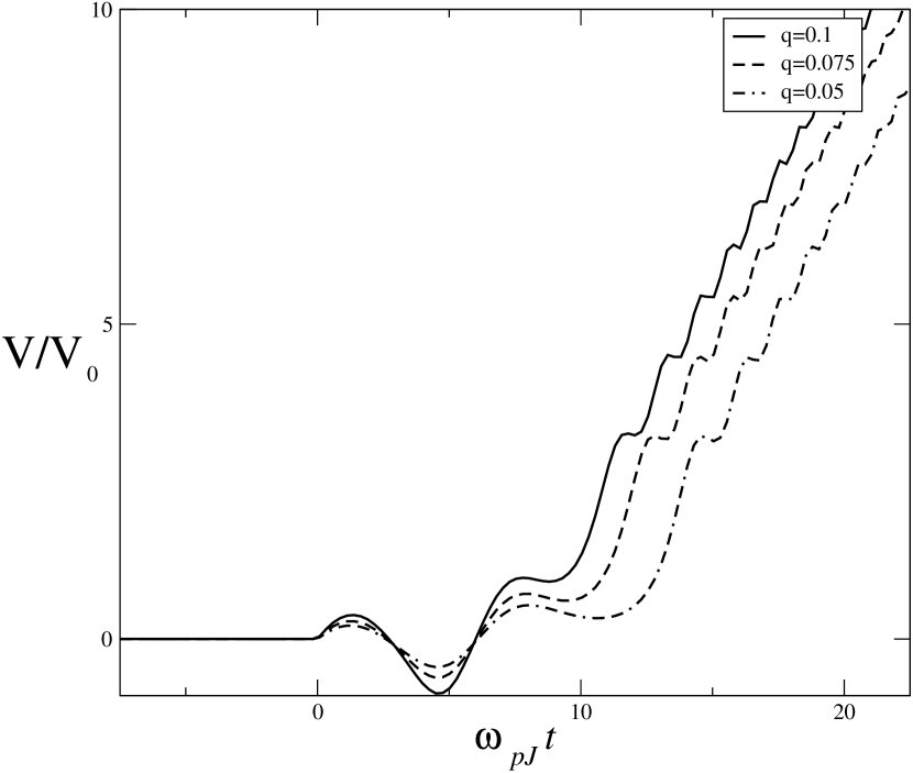
Figure 3: Voltage behavior in time for different energy released on the sample and the quality factor $Q=100$. The voltage is normalized to $V_{0}=\omega_{pJ}\varphi_{0}/c$.

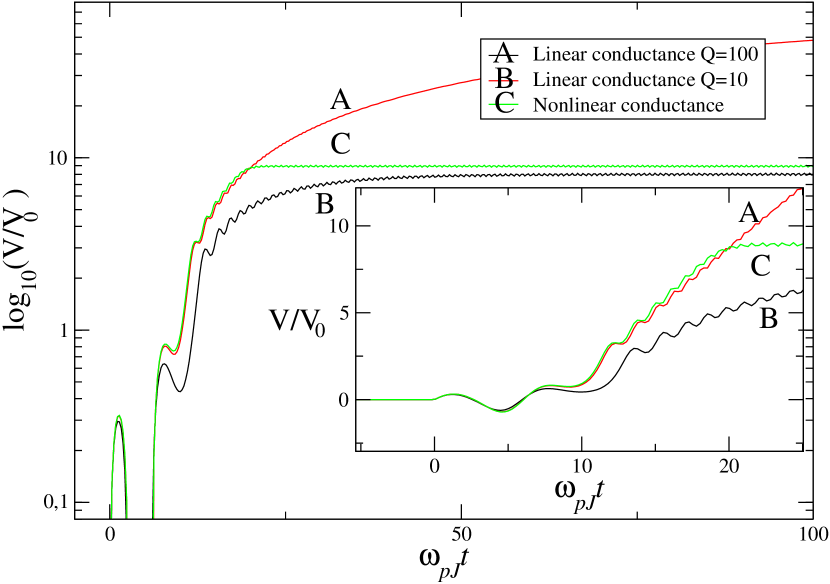
Figure 4: (Color online) Voltage behavior in time with different quality factors $Q$ in the linear conductance model (A,B) and the non-linear conductance model as given by Eq. (38) (C). The voltage is normalized to $V_{0}=\omega_{pJ}\varphi_{0}/c$.

Figure 5: Switching front in the parameter space a)$(\omega_{c}/\Delta,q)$ at fixed current bias $\gamma=J_{b}/J^{o}_{c}$ and b) $(\gamma,q)$ at fixed $\omega_{c}/\Delta$, for $Q=100$ and $\omega_{D}/\Delta=10$. The full curves have been added as a guide for the eye: they mark the border between the zero voltage (Josephson) state and the voltage state. $q$ is the coupling strength due to the laser pulse.

In Fig. (3) we show the voltage just after the pulse for different values of the released energy. The time evolution of the voltage is sketched for some successfully induced switches. The junction starts in the zero voltage state. At $\omega_{pJ}t=0^{+}$ it is irradiated by the laser pulse. There are few oscillations at frequency $\omega_{pJ}$ before the switching occurs, followed by an overall increase of the oscillating voltage. The larger is $q$ the faster is the switch. If no switch is induced the junction remains in the zero voltage state: the phase and the voltage are weakly perturbed by the radiation and show decaying plasma oscillations around their equilibrium values.

In Fig.(4) we show the approach to the gap voltage for different $Q$ values and two different conductance models. Except for the asymptotic trend, the curves for $Q=10$ (B) and $Q=100$(A) show a similar behavior. The non-linear conductance gives rise to a more pronounced shoulder in the curve after the first increase of the voltage. The first phase oscillation at frequency $\omega_{pJ}$ are largely independent of the dissipation model used.

The switching of the junction out of the zero voltage state depends on the bias current $J_{b}$, on the released energy per pulse $q$, and on the pulse duration. In Fig.(5) we sketch the switching front in the parameter space a)$(\omega_{c}/\Delta,q)$ at fixed $\gamma$ and b) $(\gamma,q)$ at fixed $\omega_{c}/\Delta$, for $Q=100$ and $\omega_{D}/\Delta=10$. For each point $(q,\omega_{c}/\Delta,\gamma)$ we calculate $J_{c}^{ad}(t)$ from Eq.s(34, 32). Next we plug the result into the equation of motion Eq. (37). Numerical simulation of the dynamics shows whether the junction is stable in the zero voltage state, or it switches to a running state. The points of the curve mark the frontier between the two behaviors. The full curve is just a guide for the eye. The non-monotonicity of $\delta\Delta(t)/\Delta$ with the pulse duration, appearing in Fig.(2) forces a similar behavior in Fig.(5$a$). This means that the pulse duration can be appropriately chosen, in order to optimize the junction switching with the laser field. Indeed, if $\omega_{c}/\Delta$ is of the order of $5\div 15$ a very small released energy is required for the switching of the junction, because the order parameter is much depressed by the laser pulse in that range. Out of this range the shorter is the pulse the larger is the energy required. By contrast a slightly larger released energy is also required for longer pulses ($\omega_{c}/\Delta<5$). This is because longer pulses imply a more extended change in the qp distribution up to higher energies. As a consequence the maximum of the function $\rho$ of Eq. 32 contributes less to the correction of the gap parameter. Nevertheless caution should be used in considering our results for longer pulses because of the neglected relaxation effects.

V Conclusion

The effect of an ultrafast laser pulse on the superconducting coherence at a Josephson Junction allows studying an unexplored regime in non equilibrium superconductivity.

Non-equilibrium in superconductivity is usually addressed in the context of one of the possible applications of Josephson junctions, that is radiation$/$particle detectors. Highly energetic radiation produces pair breaking and quasiparticles which, in turn, excite a large number of them, in a cascade process. Usually the setup is optimized such that the qp’s can be collected and contribute to the current across the junction with a sharp signal. Losses are due to degradation of the released energy into heat during the relaxation process. To achieve optimum performance, the Josephson current is usually suppressed by applying a magnetic field. This picture has been discussed quantitatively by examining the quasiclassical kinetic equation for the non equilibrium qp distribution function ovchinnikov .

In this work we have concentrated on a quite different time scale: the one fixed by the duration of an ultrafast laser pulse. While the relaxation process mentioned above takes place on a time scale of $0.1\div 100\;ns$, we have considered a laser perturbation lasting at most hundreds of femtoseconds. This type of tool can be quite valuable for future applications, because fast pulses in flux and gate voltages are extremely important when processing information in superconducting quantum computing devices (qubits) makhlin . Indeed, finite rise and fall times of pulses may result in a significant error in dynamical computation schemes choi . The carrier frequency of the laser is $\sim 100THz$ and the optical radiation is expected to produce many $e-h$ pair excitations as it would occur in a normal metal. In our case, qp’s do not have enough time to relax down to the typical phonon frequencies ($\sim\omega_{D}$) and to heat the sample before the stimulated switching occurs. We do not wish to collect qp’s either, what requires a suitable geometry of the junction.

Instead, we have addressed the question how the critical current for Josephson conduction $J_{c}$ can be coherently affected by a laser induced small perturbation with an unrelaxed non-equilibrium distribution of qp’s, that is before the dissipative response sets in.

Using the quasiclassical approach to non-equilibrium Keldysh Green’s functions, we have shown that, if the temperature is very low, the order parameter of the irradiated superconductor can respond adiabatically to a weak perturbing signal. A non equilibrium distribution of qp’s is generated and consequently $J_{c}$ is temporarily reduced (see Eq. (34) and Fig(2)). This reduction can drive switches of the junction out of the zero voltage state. In our approach the retardation effects which arise from the frequency dependence of the $e-ph$ coupling $\alpha^{2}F(\omega)$ and from the actual features of $e-ph$ relaxation processes have been neglected. They came into play on a time scale longer then the duration of the laser pulse, $\omega_{c}^{-1}\sim\tau_{c}$. Indeed in the equation of motion for the Keldysh Green’s function reported in appendix B and C the role of the frequency dependent self-energy terms has not been discussed.

The parameter which is related to the energy released by the radiation and describes the strength of the perturbation is $q$. In our case, the switches can be induced by pulses with $q\sim 0.05$, with relatively low values of $\omega_{c}/\Delta\sim 10$, by polarizing the junction very close to the critical current.

In experiments on laser induced non-equilibrium effects in superconductors testardi or Josephson junctions parker , the released energy is of few $\mu J$, which corresponds to values of $q$ between $0.25$ and $0.67$ for the given laser spot dimension. In our case for $q=0.05$ the switching occurs at 98% of the critical current. Therefore, a coherent effect of the laser on the superconducting condensate is sufficiently large to be observed in sensitive experiments monitoring the escape rate thermal ; quantum . These experiments can appreciate very small variations of the critical current, if temperature is kept low and the released energy is sufficiently small, so that sizeable heating effects do not occur.

We have also found a ‘$\cos\varphi$’ contribution to the Josephson conduction due to the presence of the excited qp’s (see Eq. (36)). This term, which will be examined in detail elsewhere, vanishes at zero $V,T$, provided excitations do not generate charge imbalance. A similar term, proportional to the voltage $V$, can be derived also in the BCS theory of Josephson conduction barone but it is identically zero as long as $V\leq 2\Delta/e$, because of the absence of qp’s at zero temperature. This is not the case here, due to the presence of a non-equilibrium qp distribution.

Our derivation of Eq.s(32,34,36) assumes that no charge imbalance is created by the perturbation. This is because the radiation excites $e-h$ pairs and the pulse duration is short enough, so that pair breaking is very limited. The absence of charge imbalance is a crucial approximation in our solution scheme. This assumption allows us to keep the unperturbed functional form of the quasiclassical Green’s functions and to insert a time dependent gap parameter $\Delta(t)$ in their expressions. $\Delta(t)$ follows the perturbation adiabatically and is determined by the non equilibrium $e-h$ pair distribution produced by the pulse. Charge imbalance corrections should be reconsidered, but they are usually expected to have a minor effect on the dynamics of the junction.

To complete the picture, we have simulated the classical dynamics of the junction switching to the resistive state. This picture is only valid over few periods $2\pi/\omega_{pJ}$ on time duration less than the electron-phonon relaxation time.

Precursor oscillations can be seen in Fig. (3) at the Josephson plasma frequency $\omega_{pJ}$. Most remarkably the duration of the pulse can be optimized in order to induce controlled coherent switching at the minimum possible released energy ${\cal{E}}$.

Appendix A Quasiclassical time dependent Green’s function approach

The quasiclassical Green’s function solve the Eilenberger form of the Gorkov equations in commutator form belzig :

$$\left[\left(\breve{G}_{0}^{-1}-\breve{\Sigma}-\breve{\Delta}\right),\breve{G}\right]_{\otimes}=0\;.$$ (39)

The matrix Green’s function $\breve{G}$ in the Keldysh space is:

$$\breve{G}=\left(\begin{array}[]{cc}\hat{G}^{R}&\hat{G}^{K}\\ \hat{0}&\hat{G}^{A}\end{array}\right)\>\>,$$ (40)

where, in turn, $\hat{G}^{R},\hat{G}^{A},\hat{G}^{K}$ are the retarded, advanced and Keldysh Green functions in the Nambu space:

$$\hat{G}^{(A,R,K)}=\left(\begin{array}[]{cc}g^{(A,R,K)}&f^{(A,R,K)}\\ -f^{(A,R,K)\dagger}&-g^{(A,R,K)\dagger}\end{array}\right)\>\;.$$ (41)

Here $f$ is the anomalous propagator and its Keldysh component defines the gap:

$$\Delta=\frac{\nu(0)\lambda}{4}\int_{-\infty}^{+\infty}d\omega\;<f^{K}>_{\vec{v}_{F}}\>.$$ (42)

The average $<>_{\vec{v}_{F}}$ denotes angular averaging over the Fermi surface. The gap matrix $\breve{\Delta}$ is defined as:

$$\breve{\Delta}\equiv\left(\begin{array}[]{cc}\hat{\Delta}&0\\ 0&\hat{\Delta}\end{array}\right)\>,\>\>\>\>\hat{\Delta}=\left(\begin{array}[]{cc}0&-\Delta\\ \Delta^{*}&0\end{array}\right)\>.$$ (43)

The self-energy $\breve{\Sigma}$ includes elastic and inelastic scattering with impurities and gives rise to relaxation processes. The commutator is evaluated w.r. to the $\otimes$ operation, which implies integration over the intermediate variables according to:

$$\breve{G}_{0}^{-1}\otimes\breve{G}_{0}\equiv\int d2\>\breve{G}_{0}^{-1}(1,2)\breve{G}(2,1^{\prime})\>,$$ (44)

where $1\equiv(\vec{r}_{1},t_{1})$. The differential operator $\breve{G}_{0}^{-1}(1,2)$ is

$$\breve{G}_{0}^{-1}(1,2)=\left[i\breve{\sigma}_{3}\partial_{t_{1}}-\frac{1}{2m}\left(\vec{\nabla}_{\vec{r}_{1}}-i\frac{e}{c}\breve{\sigma}_{3}\vec{A}(1)\right)^{2}+(e\phi(1)-\mu)\breve{I}\right]\delta(1-2)\;.$$ (45)

Here

$$\breve{\sigma}_{i}\equiv\left(\begin{array}[]{cc}\hat{\sigma}_{i}&0\\ 0&\hat{\sigma}_{i}\end{array}\right),\;\;\;\;\breve{I}\equiv\left(\begin{array}[]{cc}\hat{I}&0\\ 0&\hat{I}\end{array}\right)\;\;\;\;,$$ (46)

where $\hat{\sigma}_{i}(i=1,2,3)$ are the usual Pauli matrices and $\hat{I}$ the $2\times 2$ unit matrix .
The vector potential $\vec{A}(1)$ describes the laser radiation field of frequency $\Omega$:

$$\vec{A}(1)=\sum_{\pm}\sum_{\vec{p}}\vec{a}_{\pm}(p,t)e^{\mp i(\vec{p}\cdot\vec{r}_{1}-\Omega t)}\;,$$ (47)

where $\vec{a}_{\pm}$ can be slowly varying ’envelope’ functions of space, on the light spot size $R_{o}$ and on time, on the scale $\Omega^{-1}$. These are the reference space and time scales in the following. In the frame of the quasiclassical approximation, the original Green’s functions $G(1,2)\equiv G(\vec{r},t,\vec{r}^{\prime},t^{\prime})$ are assumed to be slowly varying function of the coordinate $\vec{R}=(\vec{r}+\vec{r}^{\prime})/2$ while they oscillate fast as functions of $\vec{r}-\vec{r}^{\prime}$ on the scale of the Fermi wavelength $\lambda_{F}$. It is customary to rewrite also the time dependence in terms of the new variables $\overline{t}=(t+t^{\prime})/2$ and $t-t^{\prime}$ and to Fourier transform $w.r.to$ $\vec{r}-\vec{r}^{\prime}$ and $t-t^{\prime}$, thus obtaining $G(\vec{p},\omega,\vec{R},\overline{t})$.
The motion equation for the Keldysh component of eq.(39) reads:

$$\left[\hat{G}_{0}^{-1}-\Re e(\hat{\Sigma})-\hat{\Delta},\hat{G}^{K}\right]_{\otimes}=\left[\hat{\Sigma}^{K},\Re e(\hat{G})\right]_{\otimes}+\frac{i}{2}\left\{\hat{\Sigma}^{K},\hat{A}\right\}_{\otimes}-\frac{i}{2}\left\{\hat{\Gamma},\hat{G}^{K}\right\}_{\otimes}\>,$$ (48)

where we have defined a quantity proportional to the density of states $\hat{A}=i(\hat{G}^{R}-\hat{G}^{A})$ (not to be confused with the vector potential), and written down the imaginary and the real part of the self-energy, $\hat{\Gamma}=i(\hat{\Sigma}^{R}-\hat{\Sigma}^{A})$ and $\Re e\hat{\Sigma}=\frac{1}{2}(\hat{\Sigma}^{R}+\hat{\Sigma}^{A})$, respectively, as well as the real part of the retarded/advanced Green’s function $\Re e\hat{G}=\frac{1}{2}(\hat{G}^{R}+\hat{G}^{A})$ ($\{,\}$ denotes the anticommutator ). The next step is the gradient expansion of the $\otimes$ product (we drop the overline on $t$ in the following):

$$\hat{C}\otimes\hat{B}=\exp{1/2(\partial^{C}_{t}\partial^{B}_{\omega}-\partial^{C}_{\omega}\partial^{B}_{t})}\exp{1/2(\partial_{p}^{C}\partial_{R}^{B}-\partial^{C}_{R}\partial_{p}^{B})}\hat{C}\hat{B}\>,$$ (49)

(here $\partial_{p}^{C}$ stands for the gradient w.r.to the impulse operating on $\hat{C}$ ), followed by the averaging of the result for $|\vec{p}|$ close to $p_{F}$, that is over the energies $p^{2}/2m-\mu\equiv\xi$ while the direction of $\vec{p}$, $\hat{p}$, is untouched:

$$\hat{g}(\hat{p},\omega,\vec{R},t)=\frac{i}{\pi}\int d\;\xi\>\>\hat{G}(\vec{p},\omega,\vec{R},t)\>\>.$$ (50)

This is justified, because $\lambda_{F}$ is much shorter both of the superconducting correlation length and of the spatial range of the laser spot ($e-h$ symmetry is assumed). Eventually $\hat{g}$ depends on $\hat{p},\omega,R,t$. The average of eq.(48) over all directions in the Fermi surface, can be done if no external bias is applied and anisotropies of the diffusion and relaxation process are not expected. In the presence of radiation with optical frequency it is customary to average out the fast oscillating components with frequency $\Omega$ landau . Following eq.(3), we expand the Green’s functions similarly:

$$\hat{\underline{g}}(\omega,R,t)={\hat{g}}(\omega,R,t)+\sum_{\pm}\hat{\chi}^{\pm}(\omega,R,t)e^{\pm i\Omega t}\;.$$ (51)

Here $\underline{\hat{g}}(\omega,R,t)$ is assumed to be the slowly varying part on the scale of the pulse duration $\tau_{c}$, while $\hat{\chi}^{\pm}$ are fast varying ones. All these functions are slowly varying functions of space as well, on the light spot size scale. A decomposition of Eq. (48) into harmonics arises. We are interested in the zero order harmonic equation, which shows a slow dynamics that can be followed coherently by the irradiated superconductor. Leaving the self-energy terms in Eq. (48) for the moment aside and dropping the superscript ^(K), we obtain

$$[\tau_{3}a_{+},\hat{\chi}^{-}]+[\tau_{3}a_{-},\hat{\chi}^{+}]+[(\omega\hat{\tau}_{3}-\hat{\Delta}),\underline{\hat{g}}]-\frac{1}{2}\{\hat{\tau}_{3},\partial_{t}\underline{\hat{g}}\}+\frac{1}{2}\{\partial_{t}\hat{\Delta},\partial_{\omega}\underline{\hat{g}}\}-\frac{e^{2}}{2mc^{2}}\partial_{t}A^{2}\partial_{\omega}\underline{\hat{g}}=...\>,$$ (52)

where the ellipsis refers to the missing self energy terms. The first order harmonic equations are:

$$\pm i\;\{\tau_{3},\hat{\chi}^{\pm}\}+\frac{e}{2mc\Omega}[a_{\pm},\underline{\hat{g}}]=0\;,$$ (53)

they show that the first two terms in Eq. (52) are ${\cal{O}}(\Omega^{-1})$ smaller than the others and can be neglected to lowest order. Hence the effective equations for the Green functions are

$$[(\omega\hat{\tau}_{3}-\hat{\Delta}),\underline{\hat{g}}]-\frac{1}{2}\{\hat{\tau}_{3},\partial_{t}\underline{\hat{g}}\}+\frac{1}{2}\{\partial_{t}\hat{\Delta},\partial_{\omega}\underline{\hat{g}}\}-\frac{e^{2}}{2mc^{2}}\partial_{t}A^{2}\partial_{\omega}\underline{\hat{g}}=...\>,$$ (54)

The last three terms in Eq. (54) include the time dependent non equilibrium dynamics that is absent in the case of a time independent approach. Retarded, advanced and Keldysh Green’s function, they all satisfy analogous equations.

Appendix B Kinetic equation for $n(\omega,r,t)$

One can linearize Eq. (54) for Keldysh Green’s function by posing $\hat{g}^{K}=\hat{g}^{R}\hat{h}-\hat{h}\hat{g}^{A}$. This yields the kinetic equation for the distribution function $n(\omega,R,t)$ scalapino . We neglect any variation in space and concentrate on the $t$ dependence here. The distribution matrix $\hat{h}$ is defined starting from the $n_{L}$ and $n_{T}$ functions according to:

$$\hat{h}=n_{L}\hat{1}+n_{T}\hat{\sigma}_{3}\>,$$ (55)

or

$$\hat{h}=\left(\begin{array}[]{cc}n_{L}(E)+n_{T}(E)&0\\ 0&n_{L}(E)-n_{T}(E)\end{array}\right)\equiv\left(\begin{array}[]{cc}1-2n(E)&0\\ 0&2n(-E)-1\end{array}\right)\>.$$ (56)

The second equality defines the relation with the qp distribution function $n(E)$. We always assume $e-h$ symmetry, so that $n(E)+n(-E)=1$ and $n_{T}=0$. In the equilibrium case one has $n_{o}(E)=\frac{1}{e^{E/T}+1}$, so that:

$$n_{L(T)}^{o}=\frac{1}{2}\left[tanh(\frac{E}{2T})+(-)tanh(\frac{E}{2T})\right]\>.$$ (57)

Substituting Eq. (19) in Eq. (54), we get the kinetic equation for the distribution matrix $\hat{h}$.In particular, in case there is no charge imbalance, the equation for the longitudinal component $n_{L}$ is ovchinnikov :

$$\partial_{t}n_{L}Tr((\hat{g}^{R}\hat{\tau}_{3}-\hat{\tau}_{3}\hat{g}^{A}))+\partial_{\omega}n_{L}Tr(\partial_{t}\hat{\Delta}(\hat{g}^{R}-\hat{g}^{A}))-\frac{e^{2}}{2mc^{2}}\partial_{t}A^{2}Tr\left(\partial_{\omega}n_{L}\left(\hat{g}^{R}-\hat{g}^{A}\right)\right)=-4I[n_{L}(\omega)]\>,$$ (58)

where $I[n_{L}(\omega)]$ is a collision integral which regulates the relaxation of the qp distribution toward equilibrium. Eq. (58) is fully discussed in ref.ovchinnikov .

Appendix C Equation of motion of $G^{R}$

We now write down the equations Eq. (54) explicitly for the retarded Green’s functions. We label the matrix components by $(i,j)\>(i,j=1,2)$ and drop the superscript ^R everywhere. The matrix elements of Eq. (52)in the Nambu space become :

$${\bf(1,1)\to} \partial_{t}g-\Delta f^{\dagger}+\Delta^{*}f+\partial_{t}\Delta\partial_{\omega}f^{\dagger}+\partial_{t}\Delta^{*}\partial_{\omega}f+\frac{e^{2}}{2mc^{2}}\partial_{t}A^{2}\partial_{\omega}g=...$$

$${\bf(2,2)\to} \partial_{t}g^{\dagger}+\Delta f^{\dagger}-\Delta^{*}f+\partial_{t}\Delta\partial_{\omega}f^{\dagger}+\partial_{t}\Delta^{*}\partial_{\omega}f-\frac{e^{2}}{2mc^{2}}\partial_{t}A^{2}\partial_{\omega}g^{\dagger}=...$$

$${\bf(1,2)\to} 2\omega f-\Delta g^{\dagger}-g\Delta+\partial_{t}\Delta\partial_{\omega}g^{\dagger}-\partial_{\omega}g\partial_{t}\Delta+\frac{e^{2}}{2mc^{2}}\partial_{t}A^{2}\partial_{\omega}f=...$$

$${\bf(2,1)\to} +2\omega f^{\dagger}-\Delta^{*}g-g^{\dagger}\Delta^{*}+\partial_{t}\Delta^{*}\partial_{\omega}g-\partial_{\omega}g^{\dagger}\partial_{t}\Delta^{*}-\frac{e^{2}}{2mc^{2}}\partial_{t}A^{2}\partial_{\omega}f^{\dagger}=...\>\>\>\>\>\>.$$

The equilibrium result suggests that

$$f=\frac{\Delta(t)}{\omega}g$$ (59)

solves Eq.$(1,2)$ except for terms $\propto\partial_{t}A^{2}$ which describe the relaxation at later times. Let us assume that this relation holds also in the non-equilibrium case. Then the formal solution, follows adiabatically the $t-$dependence of the gap parameter $\Delta$ by keeping an equilibrium-like shape:

$$g_{ad}=\frac{\omega}{\sqrt{\omega^{2}-|\Delta|^{2}(t)}},\;\;\;\;\;\;f_{ad}=\frac{\Delta(t)}{\sqrt{\omega^{2}-|\Delta|^{2}(t)}}$$ (60)

This approximate solution is quite appealing, because it satisfies the equilibrium condition for $\Delta$ at $t\to\infty$. However it neglects diffusion in space-time which will be mainly important at later times w.r. to the pulse duration.

References

- (1) A. Barone and G. Paternó, Physics and applications of Josephson effect, Wiley New York, 1982.
- (2) L. R. Testardi, Phys. Rev. B 4, 2189, 1971.
- (3) W. H. Parker and W. D. Williams, Phys. Rev. Lett. 29, 924, 1972.
- (4) C. S. Owen and D. J. Scalapino, Phys. Rev. Lett. 28, 1559, 1972.
- (5) R. A. Vardanyan and B. I. Ivlev, Sov. Phys. JEPT 38, 1156, 1974.
- (6) A.V. Sergeev, M.Yu. Reizer, J. Mod. Phys. B 6 635 (1996), M.Yu. Reizer, Phys. Rev. B 39 1602 (1989), A.V. Sergeev, M.Yu. Reizer, Zh. Eks. Teor. Fiz. 90 1096 (1986) [Sov. Phys. JETP 63 616 (1986)]
- (7) M. Lindgren, M. Currie, C. Williams, T.Y. Hsiang, P.M. Fauchet, R. Sobolewski, S.H. Moffat, R.A. Hughes, J.S. Preston, and F.A. Hegmann Appl. Phys. Lett. 74 853 (1999)
- (8) A.D. Semenov, R.S. Nebosis, Yu. Gousev, M.A. Heusinger, K.F. Renk, Phys. Rev. B 52 581 (1995).
- (9) S.B.Kaplan, C.C.Chi, D.N.Langenberg, J.J.Chuang, S.Jafarey, D.J. Scalapino, Phys.Reb.B 14, 4854, 1976.
- (10) M. H. Devoret, J. M. Martinis, D. Esteve and J. Clarke, Phys. Rev. Lett. 53, 1260, 1984.
- (11) M. H. Devoret, J. M. Martinis and J. Clarke, Phys. Rev. Lett. 55, 1908, 1985.
- (12) A.Moopenn, E.R. Arambula, M.J. Lewis, H.W. Chan, IEEE Trans. Appl. Supercond. 3, 2698, 1993,
- (13) G. P. Pepe, G. Peluso, M.Valentino, A. Barone, L. Parlato, E. Esposito, C. Granata, M. Russo, C. De Leo and G. Rotoli Appl. Phys. Lett. 79, 2770, 2001.
- (14) Superconductive Particle Detectors, edited by A.Barone (World, Singapore, 1988); A. Barone, Nucl.Phys. B 44 645 (1995).
- (15) Yu.N.Ovchinnikov and V.Z.Kresin Eur.Phys.J.B 32, 297, (2003), Yu.N.Ovchinnikov and V.Z.Kresin, Phys.Rev. B. 58,12416,(1998).
- (16) A.I.Larkin and Yu.N.Ovchinnikov Zh.Eksp.Teor.Fiz 55,2262 (1968) [Sov.Phys. JETP 28, 1200, 1969]; J.Rammer, H.Smith, Rev. Mod. Phys., 58, 323,(1986).
- (17) W.Belzig, F.K.Wilhelm, C.Bruder, G.Schoen, E.D.Zaikin Superlattices and Microstructures 25, 1251 (1999).
- (18) M.H.S.Amin, Phys.Rev.B 68 , 054505, (2003).
- (19) preliminary report on some of this material has appeared on P.Lucignano, F.J.W.Hekking and A.Tagliacozzo, in “Quantum computing and Quantum bits in mesoscopic systems”, A.J.Leggett, B.Ruggero, P.Sivestrini ed.s, Kluwer Academic, Plenum Publishers N.Y. (2004).
- (20) G.Grimvall ’The electron phonon interaction in metals’, North Holland Publ. Co. Amsterdam 1981
- (21) J.J.Chang and D.J.Scalapino, Phys.Rev.B 15 , 2651, (1977).
- (22) L.P.Gorkov and G.M.Eliashberg,Soviet Physics,JEPT27,328 (1968)
- (23) A.A.Abrikosov, L.P. Gor’kov, I.E.Dzyaloshinski, Methods of quantum field theory in statistical physics;
- (24) A. Wallraff, A. Franz, A. V. Ustinov, V. V. Kurin, I. A. Shereshevsky and N. K. Vdovicheva, PhysicaB 284-288, 575, 2000.
- (25) K. K. Likharev, Dynamics of Josephson junctions and circuits, Gordon and Breach Science Publishers, 1986.
- (26) Yu. Makhlin, G. Schön, and A. Shnirman, Rev. Mod. Phys. 73, 357 (2001)
- (27) M.S. Choi, R. Fazio, J. Siewert, and C. Bruder, Europhys. Lett. 53, 251 (2001)
- (28) L.D.Landau, E.M.Lifsits, Mechanics, Pergamon Press (1960).