Entanglement spectroscopy of a driven solid-state qubit and its detector

Abstract

We study the asymptotic dynamics of a driven quantum two level system coupled via a quantum detector to the environment. We find multi-photon resonances which are due to the entanglement of the qubit and the detector. Different regimes are studied by employing a perturbative Floquet-Born-Markov approach for the qubit+detector system, as well as non-perturbative real-time path integral schemes for the driven spin-boson system. We find analytical results for the resonances, including the red and the blue sidebands. They agree well with those of exact ab-initio calculations.

A prominent physical model to study dissipative and decoherence effects in quantum mechanics is the spin-boson model Wei . Currently, we witness its revival since it allows a quantitative description of solid-state quantum bits (qubits) Makhlin01 . A more realistic description requires the inclusion of the external control fields as well as the detector. In the spin-boson model, the environment is characterized by a spectral density $J(\omega)$. In its widest used form, $J(\omega)$ is proportional to the frequency $\omega$ mimicking the effects of an Ohmic electromagnetic environment. However, if the environment is formed by a quantum detector which itself is damped by Ohmic fluctuations, the simple Ohmic description might become inappropriate. As an example, we focus on a superconducting ring with three Josephson junctions (so termed flux-qubit). It is read out by a dc-SQUID Wal00 ; Chi03 ; Patrice04 whose plasma resonance at $\Omega_{p}$ gives rise to an effective spectral density $J_{\rm eff}(\omega)$ for the qubit with a peak at $\Omega_{p}$ Tian02 , cf.  Eq.  (4) below. Recently, the coherent coupling of a single photon mode and a superconducting charge qubit has also been studied Wallr04 . Until now, the effects of such a structured spectral density on decoherence and in presence of a resonant control field have only been studied in Thorwart00 ; Smi03 within a perturbative approach in $J_{\rm eff}$. It was shown in Tho03 ; Kle03 for the static case that a perturbative approach breaks down for strong qubit-detector coupling, and when the qubit and detector frequencies are comparable.

In the presence of microwaves, multi-photon resonances are expected to occur when the frequency of the ac-field, or integer multiples of it, match characteristic energy scales of the system Gri98 . Such multiphoton resonances can be experimentally detected in an ac-driven flux qubit by measuring the asymptotic occupation probabilities of the qubit, as the dc-field is varied Wal00 ; Saito04 . These “conventional” resonances, which have also been theoretically investigated in Goo03 , could be explained in terms of intrinsic transitions in a driven spin-boson system with an unstructured environment.

In this Letter, we investigate the asymptotic dynamics of a quantum two state system (TSS) with a structured environment, simultaneously driven by dc- and ac-fields. We show that a strong coupling between qubit and detector, together with the presence of a control field, yields a non trivial dynamics involving additional resonances in the entangled qubit+detector system. Our results are in agreement with recent experimental findings where such “unconventional” multi-photon transitions have been observed Patrice04 .

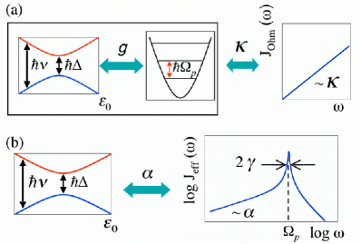
Figure 1: Schematic picture of the models we use. In ($a$) the system is a two-level-system (TSS) coupled to a harmonic oscillator with the latter coupled to an Ohmic environment with spectral density $J_{\rm Ohm}(\omega)$. In $(b)$, the TSS is coupled to an environment with peaked spectral density $J_{\rm eff}(\omega)$.

We evaluate the TSS dynamics in two completely equivalent models, cf.  Fig.  1. In model $(a)$, the TSS is coupled to its detector being represented as a single harmonic oscillator (HO) mode with frequency $\Omega_{p}$ with interaction strength $g$. The HO itself interacts with a set of harmonic oscillators, cf.  Fig. 1a. The corresponding Hamiltonian is $H_{QOB}(t)=H_{QO}(t)+H_{OB}$, where

$$H_{QO}(t) = -\frac{\hbar\Delta}{2}\sigma_{x}-\frac{\hbar\varepsilon(t)}{2}\sigma_{z}+\hbar g\sigma_{z}X+\hbar\Omega_{p}B^{\dagger}B$$

$$H_{OB} = X\sum_{k}\hbar\nu_{k}(b_{k}^{\dagger}+b_{k})+\sum_{k}\hbar\omega_{k}b_{k}^{\dagger}b_{k}\,$$ (1)

$$+X^{2}\sum_{k}\hbar\frac{\nu_{k}^{2}}{\omega_{k}}\,.$$

Here, $\sigma_{i}$ are Pauli matrices, $\hbar\Delta$ is the tunnel splitting, and $\varepsilon(t)=\varepsilon_{0}+s\cos(\Omega t)$ describes the time-dependent driving with the static bias $\varepsilon_{0}$. For $s=0$, the level splitting of the isolated TSS is $\hbar\nu=\hbar\sqrt{\varepsilon_{0}^{2}+\Delta^{2}}$. Moreover, $B$ is the annihilation operator of the localized HO mode, $X=B^{\dagger}+B$, while $b_{k}$ denote the bath mode operators. The spectral density of the continuous bath modes is Ohmic with dimensionless damping strength $\kappa$, i.e.,

$$J_{\rm Ohm}(\omega)=\sum_{k}\nu_{k}^{2}\delta(\omega-\omega_{k})=\kappa\omega\frac{\omega_{D}^{2}}{\omega^{2}+\omega_{D}^{2}}\,,$$ (2)

where we have introduced a high-frequency cut-off at $\omega_{D}$. In this approach, we shall consider the combined TSS + HO as the central quantum system.

In the second model $(b)$, we exploit the exact one-to-one mapping Garg85 of the Hamiltonian (1) onto that of a driven spin-boson Hamiltonian Gri98

$${H_{SB}}(t) = -\frac{\hbar\Delta}{2}\sigma_{x}-\frac{\hbar\varepsilon(t)}{2}\sigma_{z}$$ (3)

$$+ \frac{1}{2}\sigma_{z}\hbar\sum_{k}\tilde{\lambda}_{k}(\tilde{b}_{k}^{\dagger}+\tilde{b}_{k})+\sum_{k}\hbar\tilde{\omega}_{k}\tilde{b}_{k}^{\dagger}\tilde{b}_{k}\,,$$

where $\tilde{b}_{k}$ is the annihilation operator of the $k-$th bath mode with frequency $\tilde{\omega}_{k}$. Following Tian02 , the spectral density has a Lorentzian peak of width $\gamma=2\pi\kappa\Omega_{p}$ at the characteristic detector frequency $\Omega_{p}$. It behaves Ohmically at low frequencies with the dimensionless coupling strength $\alpha=\lim_{\omega\rightarrow 0}J_{\rm eff}(\omega)/2\omega$ and reads

$$\!\!J_{\rm eff}(\omega)=\sum_{k}\tilde{\lambda}_{k}^{2}\delta(\omega-\tilde{\omega}_{k})=\frac{2\alpha\omega\Omega_{p}^{4}}{(\Omega_{p}^{2}-\omega^{2})^{2}+(\gamma\omega)^{2}}.$$ (4)

The relation between $g$ and $\alpha$ follows as $g=\Omega_{p}\sqrt{\alpha/8\kappa}$. In this model, we associate the detector as part of the qubit environment.

The qubit dynamics is described by the reduced density operator $\rho(t)$ obtained by tracing out all environmental degrees of freedom. We study the population difference $P(t):=\langle\sigma_{z}\rangle(t)=tr(\rho(t)\sigma_{z})$ in the asymptotic limit, i.e., $P_{\infty}=\lim_{t\rightarrow\infty}\langle P(t)\rangle_{\Omega}$, where the averaging is over one period of the ac-field.

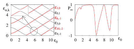
Figure 2: Left: Quasi-energy spectrum $\varepsilon_{\alpha,k}$ of the driven TSS+HO system vs dc-bias $\varepsilon_{0}$ (in units of $\Delta$). The quasi-energies are defined up to an integer multiple of $\hbar\Omega$, i.e., $\varepsilon_{\alpha,k}=\varepsilon_{\alpha}+k\hbar\Omega$. Inset: Zoom of an anti-crossing. Right: $P_{\infty}$ exhibits sidebands corresponding to quasi-energy level anti-crossings. Parameters are $\Omega=10\Delta,s=4\Delta,g=0.4\Delta,\Omega_{p}=4\Delta,\kappa=0.014$ and $k_{B}T=0.1\hbar\Delta$.

Case of weak damping and low temperatures. For $\kappa\ll 1$ and $k_{B}T\lesssim\hbar\Delta$, it is convenient to use model ($a$). The equations of motion for the TSS+HO reduced density matrix are most conveniently derived in the Floquet basis Blu89 . The Floquet states $|\phi_{\alpha}(t)\rangle=\sum_{n}|\phi_{\alpha}^{(n)}\rangle\exp(in\Omega t)$ corresponding to a periodic Hamiltonian $H(t)$ can be obtained from the eigenvalue equation ${\cal{H}}|\phi_{\alpha}(t)\rangle=\varepsilon_{\alpha}|\phi_{\alpha}(t)\rangle$, with the Floquet Hamiltonian ${\cal{H}}=H(t)-i\hbar\frac{\partial}{\partial t}$. Upon including dissipative effects to lowest order in $\kappa$, a Floquet-Born-Markov master equation is obtained Gri98 ; Kohler97 . We average the $2\pi/\Omega$-periodic coefficients over one period of the driving, assuming that dissipative effects are relevant on much larger timescales. In the Floquet basis, this yields equations of motions for $\rho_{\alpha\beta}(t)=\langle\phi_{\alpha}(t)|\rho(t)|\phi_{\beta}(t)\rangle$ of the form

$$\dot{\varrho}_{\alpha\beta}(t)=-\frac{i}{\hbar}(\varepsilon_{\alpha}-\varepsilon_{\beta})\varrho_{\alpha\beta}(t)+\sum_{\alpha^{\prime}\beta^{\prime}}L_{\alpha\beta,\alpha^{\prime}\beta^{\prime}}\varrho_{\alpha^{\prime}\beta^{\prime}}(t),$$ (5)

with the dissipative transition rates

$$L_{\alpha\beta,\alpha^{\prime}\beta^{\prime}} = \sum_{n}(N_{\alpha\alpha^{\prime},n}+N_{\beta\beta^{\prime},n})X_{\alpha\alpha^{\prime},n}X_{\beta^{\prime}\beta,-n}$$ (6)

$$- \delta_{\beta\beta^{\prime}}\sum_{\beta^{\prime\prime},n}N_{\beta^{\prime\prime}\alpha^{\prime},n}X_{\alpha\beta^{\prime\prime},-n}X_{\beta^{\prime\prime}\alpha^{\prime},n}$$

$$- \delta_{\alpha\alpha^{\prime}}\sum_{\alpha^{\prime\prime},n}N_{\alpha^{\prime\prime}\beta^{\prime},n}X_{\beta^{\prime}\alpha^{\prime\prime},-n}X_{\alpha^{\prime\prime}\beta,n}.$$

Here $X_{\alpha\beta,n}=\sum_{k}\langle\phi^{(k)}_{\alpha}|X|\phi^{(k+n)}_{\beta}\rangle$, and $N_{\alpha\beta,n}=N(\varepsilon_{\alpha}-\varepsilon_{\beta}+n\hbar\Omega)$ with $N(\varepsilon)=\frac{\kappa\varepsilon}{2\hbar}(\coth{(\frac{\varepsilon}{2k_{B}T})}-1)$ (assuming $\omega_{D}\rightarrow\infty$).

Following Ref.  Shi65 we write the Floquet Hamiltonian ${\cal{H}}_{QO}$ in the basis $|a,n\rangle$, with $|a\rangle=|g/e,m\rangle$, $g/e$ being the ground/excited state of the qubit, $m$ the oscillator state, and $n$ the Fourier index. In this basis, ${\cal H}_{QO}$ has diagonal elements ${\cal{H}}_{an,an}=\hbar[\mp\nu/2+m\Omega_{p}+n\Omega]$, and off-diagonal elements $V_{a{n},b{k}}=\langle a|\delta_{n,k}\hbar gX\sigma_{z}+(\delta_{n,k+1}+\delta_{n+1,k})\frac{\hbar s}{4}\sigma_{z}|b\rangle$. The quasi-energy spectrum of ${\cal H}_{QO}$ is shown in Fig. 2 as a function of the bias $\varepsilon_{0}$. We find avoided level crossings when $E_{an,bm}:={\cal{H}}_{an,an}-{\cal{H}}_{bm,bm}=0+O(V^{2})$, i.e., ($m\geq 0,-\infty<n<+\infty$)

$$\nu=n\Omega\pm m\Omega_{p}+O(V^{2}),\quad n\Omega=m\Omega_{p}+O(V^{2})\,.$$ (7)

Associated to the avoided crossings are resonant peaks/dips of $P_{\infty}$, see Fig. 2. The resonances at $\nu=n\Omega\pm m\Omega_{p}$ are known as red/blue sidebands Cohbook .

In the following, we derive an analytical expression for the first blue sideband at $\nu\approx\Omega-\Omega_{p}$. Other resonances can be evaluated in the same way. We include only one HO level ($m=0,1$) which is appropriate because we investigate a resonance between $|g,0\rangle$ and $|e,1\rangle$ with $g/\Omega_{p}\ll 1$. We consider $V_{an,bk}$ as a perturbation, and use the method of Ref. Cohbook ; Sha80 to obtain an effective Hamiltonian ${\cal{H}}_{\rm{eff}}=e^{iS}{\cal{H}}_{QO}e^{-iS}$, with

$$iS_{an,bm} = \left[\sum_{c,k}\frac{V_{an,ck}V_{ck,bm}}{2E_{bm,an}}\left(\frac{1}{E_{ck,an}}+\frac{1}{E_{ck,bm}}\right)\right.$$ (8)

$$+ \left.\frac{V_{an,bm}}{E_{an,bm}}\right]\mbox{ for $|E_{an,bm}|\neq|\nu+\Omega_{p}-\Omega|$},$$

and $iS_{an,bm}=0$ for $|E_{an,bm}|=|\nu+\Omega_{p}-\Omega|$. The block-diagonal ${\cal{H}}_{\rm{eff}}$ has the same eigenvalues as ${\cal{H}}_{QO}$ with quasi-degenerate eigenvalues $\varepsilon_{1,2}$ in one block. With $c_{1/3}=\frac{g^{2}}{\nu^{2}}(\frac{-\varepsilon_{0}^{2}}{\Omega_{p}}\mp\frac{\Delta^{2}}{\nu\pm\Omega_{p}})\mp\frac{\Delta^{2}s^{2}}{8(\nu^{2}-\Omega^{2})\nu}$ and $\delta=\nu-\Omega+\Omega_{p}-2c_{1}$ the quasi-energies up to second order in $V$ read

$$\varepsilon_{1/2} = -\hbar\nu/2+\hbar\delta/2\,(1\mp\sqrt{1+\Delta_{1}^{2}/\delta^{2}})+\hbar c_{1}\,,$$

$$\varepsilon_{3} = -\hbar\nu/2+\hbar\Omega_{p}-\hbar c_{3},\qquad\varepsilon_{4}=\hbar\nu/2+\hbar c_{3}.$$ (9)

The eigenvalue splitting at the level crossing, $\delta=0$, is

$$\hbar\Delta_{1}=\frac{\hbar\Delta\varepsilon_{0}gs\left[\Omega^{2}+\Omega_{p}^{2}+\nu(-\Omega+\Omega_{p})\right]}{4\nu(\Omega-\nu)\Omega\Omega_{p}(\nu+\Omega_{p})}.$$ (10)

The Floquet states are, with $\tan{\theta}=2|\Delta_{1}|/\delta$, $B^{+}(x)=\cos(x)$ and $B^{-}(x)=\sin(x)$,

$$|\phi_{1/2}\rangle = e^{-iS}[B^{\mp}{(\theta/2)}e^{-i\Omega t}|e,1\rangle\pm B^{\pm}{(\theta/2)}|g,0\rangle],$$

$$|\phi_{3}\rangle = e^{-iS}|g,1\rangle,\qquad|\phi_{4}\rangle=e^{-iS}|e,0\rangle.$$ (11)

With this, we can calculate the rates in Eq.  (6) up to second order in $V$. It holds, $L_{1122}=L_{2211}=L_{3344}=L_{4433}=0$. To find the stationary state of Eq. (5), we assume that $\rho_{\alpha\beta}(\infty)=0$ for $\alpha\neq\beta$, except for $\rho_{12}$ and $\rho_{21}$ (secular approximation). This is valid if $\varepsilon_{\alpha}-\varepsilon_{\beta}\gg L_{\alpha\beta,\alpha^{\prime}\beta^{\prime}}$, which is true for non-quasi-degenerate eigenvalues because $\kappa\ll 1$. We find at resonance

$$P_{\infty}=-\frac{\varepsilon_{0}}{\nu}\tanh\left(\frac{\hbar\Omega_{p}}{2k_{B}T}\right)+O\left(V^{2}\right),$$ (12)

implying a complete inversion of population at low temperatures. Far enough off-resonance, we can assume that $\rho_{12}(\infty)=\rho_{21}(\infty)=0$ and $\sin{(\theta/2)}\simeq\theta/2$. We presume $k_{B}T\ll\hbar\Omega_{p},\hbar\Omega,\hbar\nu$ (which allows to set $N(\hbar\Omega_{p})=N(\hbar\Omega)=N(\hbar\nu)=0$) and find the major result

$$P_{\infty} = \frac{\varepsilon_{0}}{\nu}\frac{L_{1144}-L_{4411}}{L_{1144}+L_{4411}}+O\left(V^{2}\right)$$ (13)

$$\simeq \frac{\varepsilon_{0}}{\nu}\left(1-\frac{2\Delta_{1}^{2}\nu^{2}(\nu^{2}-\Omega_{p}^{2})^{2}}{\Delta_{1}^{2}\nu^{2}(\nu^{2}-\Omega_{p}^{2})^{2}+4\Delta^{2}g^{2}\Omega_{p}^{2}\delta^{2}}\right)\!\!.\,$$

Because the oscillator can give its energy directly to the environment, the decay from $|e/g,1\rangle$ to $|e/g,0\rangle$ is much faster than the other processes and does not play a role in Eq.  (13). Hence, $P_{\infty}$ is determined by the ratio of two rates: $L_{4411}\sim\sin^{2}(\theta)\sim s^{2}g^{2}$ which describes the timescale of driving induced transitions from $|g,0\rangle$ to $|e,0\rangle$, and $L_{1144}\sim g^{2}$ for the qubit decay from $|e,0\rangle$ to $|g,0\rangle$ via the oscillator. Since both scale as $g^{2}$ we find for this particular resonance that $P_{\infty}$ is independent of $g$. Fig.  3 shows the results of Eq. (13) and different numerical results, including those of an ab-initio real-time QUAPI QUAPI calculation. A good agreement, even near resonance, is found. A similar analysis yields $P_{\infty}=\frac{\varepsilon_{0}}{\nu}\tanh({\frac{\hbar\Omega_{p}}{2k_{B}T}})+O(V^{2})$ for the first red sideband at $\nu=\Omega+\Omega_{p}$, which is very close to thermal equilibrium for low $T$. For $\nu=\Omega$ only the oscillator is excited and thermal equilibrium $P_{\infty}=\frac{\varepsilon_{0}}{\nu}\tanh({\frac{\hbar\nu}{2k_{B}T}})$ is recovered.

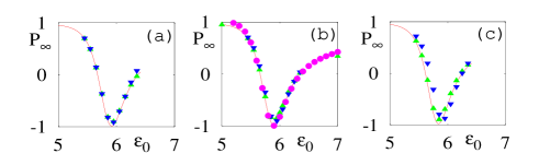
Figure 3: First blue sideband $P_{\infty}$ vs $\varepsilon_{0}$ (in units of $\Delta$) at $\nu=\Omega-\Omega_{p}$. The solid lines are the analytical prediction (13) for $(a)$ $g=0.05\Delta$, $(b)$ $g=0.2\Delta$, $(c)$ $g=0.4\Delta$. The triangles are the results of a Floquet-Bloch-Redfield simulation, cf. Eq. (5), with one (upward triangles) and two (downward triangles) HO levels taken into account. The circles in ($b$) are the results from a QUAPI simulation with six HO levels. We choose $s=2\Delta$, $\Omega=10\Delta$, $\Omega_{p}=4\Delta$, $\kappa=0.014$, $k_{B}T=0.1\hbar\Delta$.

Case of strong damping and/or high temperatures. In the complementary regime of large environmental coupling and/or high temperatures it is convenient to employ model ($b$), and is appropriate to treat the system dynamics within the noninteracting-blip approximation (NIBA) Wei . The NIBA is non-perturbative in the coupling $\alpha$ but perturbative in the tunneling splitting $\Delta$. Within the NIBA, and for large driving frequencies $\Omega>\Delta$, one finds $P_{\infty}={k_{0}^{-}}/{k_{0}^{+}}$ Gri98 , where

$$k^{\pm}_{0}=\Delta^{2}\int_{0}^{\infty}d\tau h^{\pm}(\tau)B^{\pm}(\varepsilon_{0}\tau)J_{0}\left(\frac{2s}{\Omega}\sin{\frac{\Omega\tau}{2}}\right).$$ (14)

The influence of the dc- and ac-field is in the terms $B^{\pm}(x)$, and in the Bessel function $J_{0}$, respectively. Dissipative effects are captured by $h^{\pm}(t)=e^{-Q^{\prime}(t)}B^{\pm}[Q^{\prime\prime}(t)]$, where $Q^{\prime}(t)$ and $Q^{\prime\prime}(t)$ are the real and imaginary parts of the bath correlation functionGri98 . For the peaked spectral density Eq.  (4) one finds

$$Q^{\prime}(t) = Q^{\prime}_{1}(t)-e^{-\Gamma t}[Y_{1}\cos(\bar{\Omega}_{p}t)+Y_{2}\sin(\bar{\Omega}_{p}t)]$$

$$Q^{\prime\prime}(t) = A_{1}-e^{-\Gamma t}[A_{1}\cos(\bar{\Omega}_{p}t)+A_{2}\sin(\bar{\Omega}_{p}t)]\,.$$ (15)

Here, $\beta=\hbar/k_{B}T,\Gamma=\pi\kappa\Omega_{p}$, $\bar{\Omega}_{p}^{2}=\Omega_{p}^{2}-\Gamma^{2}$ and

$$Q^{\prime}_{1}(t) = Y_{1}+\pi\alpha\Omega_{p}^{2}\left[\frac{\sinh(\beta\bar{\Omega}_{p})t}{2C\bar{\Omega}_{p}}+\frac{\sin(\beta\Gamma)t}{2C\Gamma}\right.$$ (16)

$$\left.-\frac{4\Omega_{p}^{2}}{\beta}\sum_{n=1}^{\infty}\frac{\frac{1}{\nu_{n}}[e^{-\nu_{n}t}-1]+t}{(\Omega_{p}^{2}+\nu_{n}^{2})^{2}-4\Gamma^{2}\nu_{n}^{2}}\right],$$

where $\nu_{n}=2\pi n/\beta$. Moreover, $C=\cosh(\beta\bar{\Omega}_{p})-\cos(\beta\Gamma)$, $CY_{1/2}=\mp A_{2/1}\sinh\beta\bar{\Omega}_{p}-A_{1/2}\sin\beta\Gamma$, $A_{2}=\alpha\pi(\Gamma^{2}-\bar{\Omega}_{p}^{2})/2\Gamma\bar{\Omega}_{p}$, $A_{1}=\pi\alpha$. So, $Q^{\prime}$ and $Q^{\prime\prime}$ display damped oscillations (cf. Fig. 4) not present for a pure Ohmic spectrum. It is the interplay between these oscillations and the driving field which induces the extra resonances in $P_{\infty}$. In the regime $\Gamma/\Omega_{p}\ll 1$, the term $\exp(-\Gamma t)$ in Eq.  (16) varies slowly on the time-scale of the oscillations. We expand $Q^{\prime}$ and $Q^{\prime\prime}$ as well as the Bessel function $J_{0}$ entering (14) using Bessel function identities and find the important result

$$k_{0}^{\pm}=\sum_{m=0}^{\infty}\sum_{n=-\infty}^{\infty}\Delta^{2}\int_{0}^{\infty}dte^{-Q_{1}^{\prime}(t)}f^{\pm}_{mn}(t)\;,$$ (17)

where $\varepsilon_{mn}=\varepsilon_{0}-m\bar{\Omega}_{p}-n\Omega$, and

$$f^{\pm}_{mn}(t)={{\rm Re}\atop{\rm Im}}\left[{c^{\pm}_{mn}(t)\cos(\varepsilon_{mn}t)\pm c^{\mp}_{mn}(t)\sin(\varepsilon_{mn}t)}\right],$$

$$c^{\pm}_{mn}=J_{n}^{2}\left(\frac{s}{\Omega}\right)J_{m}(e^{-\Gamma t}\omega_{1})B^{\pm}(m\phi)(-i)^{m}e^{-iA_{1}}\,.$$ (18)

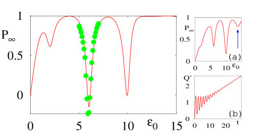
Figure 4: $P_{\infty}$ vs $\varepsilon_{0}$ (in units of $\Delta$). The solid line is the NIBA prediction, while the circles are from a QUAPI simulation with 6 HO levels ($g=3\Delta$, $s=4\Delta$, $\Omega=10\Delta$, $\kappa=0.014$, $k_{B}T=0.5\hbar\Delta$, $\Omega_{p}=4\Delta$). Inset ($a$): NIBA result for $k_{B}T=2\hbar\Delta$. The arrows indicates the first red sideband at $\nu=\Omega+\Omega_{p}$. Inset ($b$): $Q^{\prime}(t)$ vs $t$ shows damped oscillations.

Here is $\omega_{1}=\sqrt{(A_{1}-iY_{1})^{2}+(A_{2}-iY_{2})^{2}}$, and $\tan\phi=-({A_{2}-iY_{2}})/({A_{1}-iY_{1}})$. Thus, from Eq. (Entanglement spectroscopy of a driven solid-state qubit and its detector) we expect resonances when $\varepsilon_{nm}=0$. Without driving we always find that around $\varepsilon_{0}=m\bar{\Omega}_{p}$ it holds $P_{\infty}\approx\tanh({m\beta{\Omega}_{p}/2)}$, since $\lim_{\Gamma/\Omega_{p}\rightarrow 0}\tan(m\phi)=i\tanh(m\beta\Omega_{p}/2)$ (for not too large $T$, i.e., $\cos(\beta\Gamma)\ll\cosh(\beta\Omega_{p})$). Hence, $P_{\infty}$ acquires its NIBA thermal equilibrium value, and driving is needed to see resonances. For “conventional” resonances at $\varepsilon_{0}=n\Omega$ we find $P_{\infty}\approx 0$, as predicted for unstructured environments Har00 ; Goo03 . Finally, for $\varepsilon_{0}=n\Omega\pm m\bar{\Omega}_{p}$, we recover $P_{\infty}\approx\pm\tanh(m\beta\Omega_{p}/2)$, as also was found within the Floquet-Born-Markov approach, cf. (12). Results of a numerical evaluation of $P_{\infty}$ are shown in Fig. 4, using the NIBA result (Entanglement spectroscopy of a driven solid-state qubit and its detector), as well as the exact ab-initio real-time QUAPI method QUAPI . In the numerical evaluation, we could not reach the parameter regime $\Gamma/\Omega_{p}\ll 1$, but still clear resonance dips are observed at $\varepsilon_{0}=\Omega$, $\varepsilon_{0}=\Omega-\Omega_{p}$ and $\varepsilon_{0}=\Omega-2\Omega_{p}$. For $k_{B}T\sim\hbar\Omega_{p}$, we also find the first red sideband at $\varepsilon_{0}=\Omega+\Omega_{p}$, see inset.

In conclusion we evaluated the asymptotic population of a driven TSS in a structured environment. We have derived analytic expressions for the shape of the resonances for both weak and strong damping. We show that the coupling of the TSS and the detector is revealed in the occurrence of characteristic multi-photon resonances, also reported in recent experiments Patrice04 , in the asymptotic population of the TSS. A complete population inversion is predicted for the blue-sidebands transitions, while values close to equilibrium are found for the red-sidebands.

Support by the Dutch NWO/FOM, and the Universitätsstiftung Hans Vielberth, and discussions with P. Bertet, I. Chiorescu and H. Mooij are acknowledged.

References

(1) U. Weiss, Quantum Dissipative Systems
(World Scientific, Singapore, 1999).
(2) Y. Makhlin, G. Schön and A. Shnirman, Rev. Mod. Phys. 73, 357
(2001).
(3) C. van der Wal et al., Science 290, 773 (2000).
(4) I. Chiorescu et al., Science 299, 1869 (2003).
(5) I. Chiorescu et al., Nature 431, 159 (2004).
(6) L. Tian, S. Lloyd, T.P. Orlando, Phys. Rev. B
65, 144516 (2002).
(7)A. Wallraff et al., Nature 431, 162 (2004).
(8)M. Thorwart et al.,
J. Mod. Opt. 47, 2905 (2000).
(9) A. Yu. Smirnov, Phys. Rev. B 67, 155104 (2003).
(10) M. Thorwart, E. Paladino and M. Grifoni, Chem. Phys. 296, 333 (2004).
(11) F. K. Wilhelm, S. Kleff and J. von Delft,
Chem. Phys. 296, 345 (2004).
(12) M. Grifoni and P. Hänggi, Phys. Rep. 304, 229 (1998).
(13) S. Saito et al., Phys. Rev. Lett. 93, 037001 (2004).
(14) M. C. Goorden and F. K. Wilhelm, Phys. Rev. B 68, 012508 (2003).
(15)A. Garg, J. N. Onuchic and V. Ambegaokar,
J. Chem. Phys. 83, 4491 (1985).
(16) R. Blümel et al., Phys. Rev. Lett. 62, 341 (1989).
(17) S. Kohler, T. Dittrich, and P. Hänggi,
Phys. Rev. E 55, 300 (1997).
(18) J.H. Shirley, Phys. Rev. 138, B979 (1965).
(19) C. Cohen-Tannoudji, J. Dupont-Roc and G. Grynberg,
Atom-Photon Interactions (Wiley, New York, 1992).
(20) I. Shavit and L. T. Redmon, J. Chem. Phys. 73, 5711 (1980).
(21) N. Makri and D.E. Makarov, J. Chem. Phys. 102, 4600 (1995).
(22) L. Hartmann et al., Phys. Rev. E 61, R4687 (2000).