Lattice Boltzmann model with hierarchical interactions

Abstract

We present a numerical study of the dynamics of a non-ideal fluid subject to a density-dependent pseudo-potential characterized by a hierarchy of nested attractive and repulsive interactions. It is shown that above a critical threshold of the interaction strength, the competition between stable and unstable regions results in a short-ranged disordered fluid pattern with sharp density contrasts. These disordered configurations contrast with phase-separation scenarios typically observed in binary fluids. The present results indicate that frustration can be modelled within the framework of a suitable one-body effective Boltzmann equation. The lattice implementation of such an effective Boltzmann equation may be seen as a preliminary step towards the development of complementary/alternative approaches to truly atomistic methods for the computational study of glassy dynamics.

PACS: 47.11.+j, 05.70.Fh, 64.75.+g
Keywords: Lattice Boltzmann equation, computer simulations, phase transition
^a Corresponding author E_mail: a.lamura@area.ba.cnr.it Phone: +39 0805530719 Fax: +39 0805588235

I Introduction

A deeper understanding of the behavior of disordered systems, and notably glassy ones, represents an outstanding challenge in modern condensed matter physics. In the face of the lack of a comprehensive theory, much work is currently devoted to the numerical simulation of glassy behavior. To date, these simulation efforts rely mainly on Molecular Dynamics and Monte Carlo techniques [1, 2]. Both methods incorporate details of microscopic behavior (intermolecular potentials) and, as a result, they fall short of reaching spatio-temporal scales of macroscopic interest. A typical molecular dynamics simulation would last a few tens-hundreds of nanoseconds, to be contrasted with relaxation times of the order of an hour and more of real glasses. Larger scales are made accessible by coarse-grained lattice gas models in which the details of true molecular interactions are replaced by suitable heuristics about the behavior of fictitious lattice molecules. These models reach out larger scales but the corresponding outcomes have to be critically weighted against the simplifying assumptions they are based upon. At the extreme of this line one finds spin-glasses [3, 4] and their modern lattice glass variants [5, 6].

Although to a different degree of physical fidelity, all of these models retain the many-body nature of the intermolecular interactions, with an inevitable price in terms of computational effort. It is therefore of great interest to explore whether mesoscopic models, namely suitable effective one-body formulations may capture at least some basic features of glassy behavior, at a fraction of the computational cost associated with the aforementioned many-body simulation techniques.

In the present paper this task is pursued within the framework of the lattice Boltzmann equation (LBE), a minimal kinetic equation describing stylized pseudo-molecules evolving in a regular lattice according to a simple local dynamics including free-streaming, collisional relaxation and (effective) intermolecular interactions [7, 8, 9]. In particular, we shall show that it is possible to construct a class of suitable mesoscopic potentials supporting some basic traits of disordered systems. Here we shall focus on a minimal requirement: The ability to sustain sharp density contrasts within a disordered pattern.

The paper is organized as follows. In the next Section, after a cursory view of the main features of the standard LBE, we present our model. Section III is devoted to the results of numerical simulations and finally, we discuss the main findings of the present paper and outline possible future research directions.

II The model

The most popular form of lattice Boltzmann equation (Lattice BGK, for Bhatnagar, Gross, Krook) [10], reads as follows:

$$f_{i}(\vec{r}+\vec{c}_{i},t+1)-f_{i}(\vec{r},t)=-\omega[f_{i}-f_{i}^{e}](\vec{r},t)$$ (1)

where $f_{i}(\vec{r},t)\equiv f(\vec{r},\vec{v}=\vec{c}_{i},t)$ is a discrete distribution function of particles moving along with discrete speed $\vec{c}_{i}$. The right-hand side represents the relaxation to a local equilibrium $f_{i}^{e}$ in a time lapse of the order of $\omega^{-1}$. This local equilibrium is usually taken in the form of a quadratic expansion of a local Maxwellian:

$$f_{i}^{e}=\rho w_{i}[1+\frac{\vec{u}\cdot\vec{c}_{i}}{c_{s}^{2}}+\frac{\vec{u}\vec{u}\cdot(\vec{c}_{i}\vec{c}_{i}-c_{s}^{2}I)}{2c_{s}^{4}}]$$ (2)

where $\rho=\sum_{i}f_{i}$ is the fluid density, $\rho\vec{u}=\sum_{i}f_{i}\vec{c}_{i}$ the fluid current, $w_{i}$ is a set of weights normalized to unity, $c_{s}$ the lattice sound speed (a constant equal to $1/\sqrt{3}$ in our case) and finally, $I$ stands for the unit tensor. The set of discrete speeds must be chosen in such a way as to guarantee mass, momentum and energy conservation, as well as rotational invariance. Only a limited subclass of lattices qualifies. In the sequel, we shall refer to the nine-speed lattice consisting of zero-speed, speed one $c=1$ (nearest-neighbor connection), and speed $c=\sqrt{2}$, (next-nearest-neighbor connection). Standard analysis shows that the LBE system behaves like a quasi-incompressible fluid with an ideal equation of state $p=\rho c_{s}^{2}$ and kinematic viscosity $\nu=c_{s}^{2}(1/\omega-1/2)$. Departures from ideal-gas behavior within the LBE formalism are typically described by means of phenomenological pseudo-potentials mimicking the effects of potential energy interactions [11]. These pseudo-potentials have proved capable of describing a wide range of complex fluid behaviors, such as phase-separation in binary fluids and phase-transitions. To date, however, no LBE model appears to have addressed frustrated systems. This is precisely the scope of this work.

We choose the empirical pseudo-potential in the form of a lattice-truncated repulsive Lennard-Jones interaction:

$$V(r) = G\Psi(\rho)(r/\sigma)^{-12},\;\;\;1<r<\sqrt{2}$$ (3)

$$V(r) = 0,\;\;\;\;\;\;\;\;\;\;\;\;\;\;\;\;\;\;\;\;\;\;\;\;\;\;\;\;elsewhere$$ (4)

where the cut-off $\sigma=1$ in lattice units and $G$ is a parameter controlling the strength of the interaction (an inverse effective temperature), hence the surface tension between dense and light phases. The density-dependence is taken in the form of a hierarchy of polynomials, whose density zeroes are distributed according to a binary tree of depth $N_{g}$ (number of generations):

$$\Psi(\rho)=(\rho-\rho_{0})\;\prod_{g=2}^{N_{g}}\frac{-1}{(1+(\frac{\rho-\rho_{0}}{\delta\rho_{0}/2})^{2^{g-1}})^{2}}\prod_{k=1}^{2^{g-1}}\frac{(\rho-\rho_{gk})}{(\rho_{gk}-\rho_{0})}$$ (5)

where $\delta\rho_{0}$ is the typical scale for the density gap. Starting with the root value $\rho_{0}$, at each generation $g$, a mother density $\rho_{gk}$ spawns two children $\rho_{g+1,2k},\rho_{g+1,2k+1}$ spaced by an amount $\pm\delta\rho_{0}/2^{g-1}$ away from the mother value. This hierarchical potential implements the presence of $N_{\rho}=2^{N_{g}}-1$ competing density extrema.

As an example, for $N_{g}=3$,

$$g=1 : \rho_{0}$$ (6)

$$g=2 : \rho_{1,2}=\rho_{0}(1\mp\delta\rho_{0}/2)$$ (7)

$$g=3 : \rho_{3,4,5,6}=\rho_{0}(1\mp\delta\rho_{0}/2\mp\delta\rho_{0}/4)$$ (8)

The denominator serves the purpose of letting $\Psi\rightarrow 0$ outside the hierarchical range of zeroes $\rho_{gk}$. The result is an effective potential alternating stable repulsive regions ($\Psi^{\prime}>0$, prime meaning derivative with respect to $\rho$) with unstable attractive ones ($\Psi^{\prime}<0$), distributed approximately in the density range $\rho_{\mp}=\rho_{0}(1\mp\delta\rho_{0}(1-2^{-N_{g}}))$. Since the case $N_{g}=2$ (cubic interaction) is somewhat equivalent to a Van der Waals interaction, we can think to our potential as of a series of hierarchically nested van der Waals interactions. It is intuitively clear that if the coupling strength $G$ is sufficiently strong, attractive regions are subject to instabilities which can be likened to a phase transition. However, since there are multiple forbidden regions interweaved with density gaps with (meta)stable behavior, the system is amenable to a full cascade of phase-transitions, depending on the strength of the interaction. As a result, the fluid is expected to exhibit a sort of “frustration” resulting from the competition of the multiple density minima. This competition is resolved through steep interfaces connecting the stable density regimes. In the language of free-volume theory, this frustration relates to the disordered short-range coexistence of two competing species: “voids” (regions with $\rho<\rho_{0}$) and “cages” (regions with $\rho>\rho_{0}$). This contrasts with binary separation scenarios, in which the two species organize over coherent patterns (“blobs”) of sizeable extent.

The LBE with hierarchical interactions takes the final form

$$f_{i}(\vec{r}+\vec{c}_{i},t+1)-f_{i}(\vec{r},t)=-\omega[f_{i}-f^{eq}_{i}](\vec{r},t)+F_{i}[\rho(\vec{r},t)]$$ (9)

where $F_{i}=-G\frac{\rho}{\rho_{0}}\nabla\Psi[\rho]\cdot\vec{c}_{i}$. This can be regarded as a dynamic, mean-field model of a non-ideal fluid with multiple density phases.

III Numerical simulations

To assess the viability of the present LBE, we have simulated a 2D dimensional fluid with the following parameters: Grid size $256\times 256$, $\omega=1.0$, $\rho_{0}=1.0$, $N_{g}=3$, $\delta\rho_{0}=0.5$, and $G$ is varied between $0$ and $1.0$. The resulting effective potential $\Psi(\rho)$ is shown in Fig. 1. The initial condition is $\rho(x,y)=\rho_{0}\;(1+\xi)$ where $\xi$ is a random perturbation uniformly distributed in the range $[-0.01:0.01]$. Due to the combined effect of kinetic hopping from site to site (the left-hand-side of the LBE) and mode-mode coupling [12] induced by the non-linear potential $\Psi(\rho)$, the density distribution spreads out in time, so that an instability is triggered as soon as $G$ exceeds the critical threshold $G_{c}$. In Fig. 2 we show the maximum and minimum densities as a function of the coupling strength $G$. This Figure highlights a sizeable symmetry breaking of the order of $\Delta\rho/\rho>1$ for $G>G_{c}$, where $\Delta\rho=\rho_{max}-\rho_{min}$. The density gap $\Delta\rho$ starts up at $G=G_{c}\sim 0.09$ and rapidly fills the available range of states between $\rho_{-}$ and $\rho_{+}$, as the interaction strength is increased. The scaling law is approximately $\Delta\rho\sim(G-G_{c})^{1/2}$ in accordance with mean-field theory. The critical value estimated on the basis of the stability condition

$$|\Psi^{\prime}|>c_{s}^{2}/G$$ (10)

yields $G_{c}\sim 0.089$, in a nice agreement with numerical data. A similar message is sent by the order parameter $M=\sqrt{<(\delta\rho)^{2}>}/<\rho>$, where $\delta\rho\equiv\rho-<\rho>$ is the density fluctuation around its spatial average, which is represented by the dotted line in Fig. 2. Inspection of the spatial distribution of the density field $\rho(x,y)$ shows that this non-zero order parameter is not associated with phase-separation, but rather with a disordered coexistence of voids and cages (see Fig. 3). This shows that the potential allows to model sharp density contrasts over a disordered spatial distribution.

As a further observable, in Fig. 4 we plot the density-density correlation:

$$g(r)=\frac{<\delta\rho(x+r_{x},y+r_{y})\delta\rho(x,y)>}{<\rho(x,y)\rho(x,y)>},$$ (11)

where $r^{2}=r_{x}^{2}+r_{y}^{2}$. The curve has been obtained upon averaging the quantities $g(r)$ over ten independent runs with different initial configurations. The error bars show the maximum errors on the values $g(r)$ at each value of $r$. This function exhibits oscillating-decay behavior. Being in a lattice, it is clear that data are only available at discrete positions $1,\sqrt{2},2,\dots$. The small error bars and the non-oscillating behavior of $g(r)$ in the absence of potential, which is virtually zero as a consequence of the uniform and constant density distribution, suggest that the observed oscillations in the case $G\neq 0$ are not a numerical artifact. However, only further simulations of larger systems can confirm this result.

In order to look for the existence of slow relaxation modes, we computed the density-density time-correlation function $h(\tau)$ (see Fig. 5)

$$h(\tau)=\frac{<\delta\rho(x,y,t+\tau)\delta\rho(x,y,t)>_{t}}{<\rho(x,y,t)\rho(x,y,t)>_{t}}$$ (12)

taken at $x=128,y=128$. In the above, $<...>_{t}$ denotes a time average. We have run ten independent simulations starting from different initial configurations, and we computed $h(\tau)$ in each run. These individual quantities were first averaged over time intervals of $150$ time-steps in order to eliminate high frequencies, and then the final average over the ten runs was taken. These quantities are plotted in Fig. 5 where the error bars represent the maximum error on the values of $h(\tau)$. We find persistent oscillations around zero, possibly reflecting an everlasting competition between the various density minima of the potential over the timescale of the simulation. The case $G=0$ shows an immediate decay to zero of the time-correlation function, reflecting the fast relaxation towards a uniform distribution when no potential is acting on the system.

IV Conclusions

We have presented a new mesoscopic lattice Boltzmann model with a density-dependent hierarchy of attractive and repulsive interactions. The long-time dynamics of this model yields disordered patterns with sharp short-range density contrasts, as opposed to binary phase-separation scenarios. Such configurations do not relax towards a frozen state, but continuously change preserving a disordered spatial structure. The present results show that one distinguishing feature of disordered behavior, namely frustration, can be modeled within the framework of a suitable one-body effective kinetic theory. On the other hand, the same results also show that further crucial signatures of glassy behavior, such as slow time-relaxation, are not captured by the present hierarchical model. At this point, the main question is: what major ingredients of glassy dynamics are we missing in the present model?

According to Palmer et al [13], a successfully theory of glassy relaxation should satisfy three basic requirements: (1) The theory must be based on dynamics, and not just statistics, because since glasses break ergodicity, equilibrium distributions are of scanty use. (2) The above dynamics must be constrained, because there is no reasonable hope to diagonalize such highly non-linear systems into independent modes. And finally, (3) the theory should be hierarchical, so that slow modes can adiabatically enslave the fast ones, while the fast modes, in return, set constraints on the dynamics of the slow ones.

Our hierarchical LB model does indeed generically meet with all of these three requirements, but only incompletely. The model is dynamic, but nonetheless based on a single-time relaxation to local equilibrium. Our model is also non-linear and hierarchically constrained, but still within the class of effective one-body theories. Such effective one-body theories prove exceedingly successful for simple fluids, but it might be that the physics of glasses, and particularly dynamic inhomogeneity [14, 15], is just too intimately related to many-body effects which are beyond the reach of effective mean field theories, no matter how ingenious. We believe that, independently of the computational pay-offs discussed earlier in this work, this latter question bears a significant theoretical interest on its own. Work in this direction is currently underway.

Acknowledgments
We thank Professors E. Marinari and G. Parisi for many illuminating comments and discussions. SS wishes to thank Prof. K. Binder for valuable discussions and for bringing Ref. [1] to his attention.

FIG. 1.: The pseudo-potential $\Psi(\rho)$ for the case $N_{g}=3$, $\rho_{0}=1.0$, $\delta\rho_{0}=0.5$.

FIG. 2.: The maximum (full line) and minimum (dashed line) densities and the order parameter $M$ (dotted line) as a function of the coupling strength $G$.

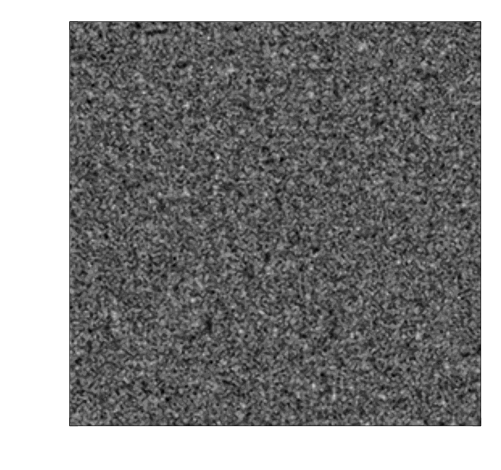
FIG. 3.: Snapshot of the density configuration at $t=200$ for the case $G=0.45$. Black/white colors code for high/low density.

FIG. 4.: Density-density correlation function at $t=200$ for the cases $G=0$ ($\ast$) and $G=0.45$ ($\bullet$), averaged over ten independent runs. Error bars are shown for the case $G=0.45$.

FIG. 5.: Density-density time correlation function for the cases $G=0$ (dashed line) and $G=0.45$ (full line), averaged over ten independent runs. Error bars are shown for the case $G=0.45$.

REFERENCES

- [1] K. Binder, Progress in polymer science, 2002, in press.
- [2] M. Mézard and G. Parisi, J. Phys. Cond. Matt. 12, 6655 (2000).
- [3] K. Binder and A. P. Young, Rev. Mod. Phys. 58, 801 (1986).
- [4] M. Mézard, G. Parisi, and M. Virasoro, Spin glass theory and beyond, World Scientific, Sigapore, (1987).
- [5] J.P. Bouchaud, L. Cugliandolo, J. Kurchan, and M. Mézard, Spin glasses and random fields, A.P. Young editor, World Scientific, Sigapore, (1998).
- [6] G. Biroli and M. Mezard, Phys. Rev. Lett. 88, 025501 (2002).
- [7] R. Benzi, S. Succi, and M. Vergassola, Phys. Rep. 222, 145 (1992); D. A. Wolf-Gladrow, Lattice Gas Cellular Automata and Lattice Boltzmann models, Springer Verlag, (2000); S. Succi, The Lattice Boltzmann equation, Oxford University Press, Oxford, (2001).
- [8] Proceedings of the 9th Int. Conf. on the Discrete Simulation of Fluids, J. Stat. Phys, 107 (1-2), (2002).
- [9] W. Miller, S. Succi, and D. Mansutti, Phys. Rev. Lett. 86, 3578 (2001).
- [10] Y. Qian, D. d’Humières, and P. Lallemand, Europhys. Lett. 17, 479 (1992).
- [11] X. Shan and H.Chen, Phys. Rev. E 47, 1815 (1993); Phys. Rev. E 49, 2941 (1994).
- [12] W. Goetze, J. Phys: Condens. Matter 11, A1 (1999).
- [13] R. G. Palmer, D. L. Stein, E. Abrahams and P. W. Anderson, Phys. Rev. Lett. 53, 958 (1984).
- [14] D. Caprion, J. Matsui, and H. R. Schober, Phys. Rev. Lett. 85, 4293 (2000).
- [15] J. P. Garrahan and D. Chandler, Phys. Rev. Lett. 89, 035704 (2002).