Spin relaxation dynamics of quasiclassical electrons in ballistic quantum dots with strong spin-orbit coupling

Abstract

We performed path integral simulations of spin evolution controlled by the Rashba spin-orbit interaction in the semiclassical regime for chaotic and regular quantum dots. The spin polarization dynamics have been found to be strikingly different from the D’yakonov-Perel’ (DP) spin relaxation in bulk systems. Also an important distinction have been found between long time spin evolutions in classically chaotic and regular systems. In the former case the spin polarization relaxes to zero within relaxation time much larger than the DP relaxation, while in the latter case it evolves to a time independent residual value. The quantum mechanical analysis of the spin evolution based on the exact solution of the Schrödinger equation with Rashba SOI has confirmed the results of the classical simulations for the circular dot, which is expected to be valid in general regular systems. In contrast, the spin relaxation down to zero in chaotic dots contradicts to what have to be expected from quantum mechanics. This signals on importance at long time of the mesoscopic echo effect missed in the semiclassical simulations.

I I Introduction

Spin relaxation in semiconductors is an important physical phenomenon being actively studied recently in connection with various spintronics applications reviewonsptronics . In doped bulk samples and quantum wells (QW) of III-V semiconductors at low temperatures spin relaxation is mostly due to the DP mechanism DP . This mechanism does not involve any inelastic processes, so that the exponential decay of the spin polarization is determined entirely by the spin-orbit interaction (SOI) and elastic scattering of electrons on the impurities. However, in case of confined systems such as quantum dots (QD) with atomic-like eigenstates, the SOI has been incorporated into the structure of the wave functions of the discrete energy levels. Without inelastic interactions, an initial wave packet with a given spin polarization will evolve in time as a coherent superposition of these discrete eigenstates. Therefore, the corresponding expectation value of the spin polarization will oscillate in time without any decay. To obtain a polarization decay in the QD’s, extra effects have to be introduced into the system, e.g., the inelastic interactions between electrons and phonons mediated by the spin-orbit Khaetskii ; Woods and nuclear hyperfine effects Khaetskii ; Merkulov ; Semenov . Accordingly, a spin relaxation in QD’s induced by these effects is a real dephasing process.

Unlike such an inelastic relaxation in QD’s, the DP spin relaxation in unbounded systems seems to be a quite different phenomenon, because the scattering on impurities is elastic and there is no dephasing of the electron wave functions in the systems. However, the spin polarization does decay in time exponentially, as if it would be a true dephasing process. To explain this phenomenon, let us consider an electron moving diffusively through an unbounded system with random elastic scatters. This electron is described by a wave packet represented by a superposition of continuum eigenstates. During a DP relaxation process, the spin expectation value expressed as a bilinear combination of these wave amplitudes will decay exponentially in time. This process can be easily understood from the semiclassical Boltzmann or Fokker-Plank approach DP . Indeed, keeping in mind that the SOI has the form $\bm{\sigma}\cdot\mathbf{h(k)}$, where $\bm{\sigma}$ is the vector, whose components are the three Pauli matrices, and $\mathbf{h(k)}$ is the effective magnetic field, whose magnitude and direction depend on the electron momentum $\mathbf{k}$, one can envision spin relaxation as the spin random walk on the surface of the unit sphere, similar to that in Fig. 1(c). Starting at the north pole, the spin precesses around $\mathbf{h(k_{1})}$ until the momentum direction is changed by a scattering on an impurity. Thereafter, the magnetic field changes its direction to $\mathbf{h(k_{2})}$ and the spin continues its precession around this new direction. If the spin rotation angle between successive scattering events is small, the sequence of such rotations results in a diffusive spreading of the initial polarization.

Returning to QD’s, a natural question emerges: what sort of spin evolution can be generated by the DP mechanism in a ballistic QD whose size is much larger than the electron wavelength at the Fermi surface and where the mean spacing between energy levels is much less than $\hbar/T$, where $T$ is the mean time between electron collisions with the boundary? Similar to the example in Fig. 1, the spin evolution in this semiclassical regime can be studied by tracking the spin walk on the sphere, when particles move along the classical trajectories inside the QD’s. Intuitively, one would expect the spin evolution in this case to be similar to the spin random walk governed by the impurity scattering in unbounded samples. However, this expected analogy with the open system is wrong. Indeed, in an unbounded system, the steps of the random walk are uncorrelated. This results in a diffusive decay of the spin polarization down to zero for any nonzero SOI. But in case of QD’s, the steps of the random walk on the sphere are correlated due to the confinement of electron trajectories within the dots. As we will show below, such correlations not only lead to a spin relaxation much longer than the DP relaxation in unbounded systems, but also to a non-zero final polarization value at long time for certain quantum dot geometries. Here, we do not take into account the inelastic mechanisms Khaetskii ; Merkulov ; Semenov ; Woods which always drive the spin polarization to zero in long time. These mechanisms are assumed to be absent, because they become inefficient at low sufficiently temperatures.

In this article we carry out a semiclassical analysis of the DP relaxation in 2-dimensional (2D) QD’s of various geometries, including a circular dot, a triangular dot, a generalized Sinai billiard, and a circular dot with diffusive scattering on the boundary. We focus on the case of the strong SOI, such that the characteristic spin orbit length $L_{so}\equiv v_{F}/\hbar h(\bm{k_{F}})$ is not much larger than the dot size $L$. Such a regime can be realized in the InAs based heterostructures for $L\sim 0.5-1\mu m$ Nitta . We found that in the short time scale $\sim T$ the spin relaxation dynamics in all geometries shares a common feature: After a fast initial drop during the time interval $\sim T$, the spin polarization continues to oscillate weakly around some value. For weak SOI with $L_{so}\gg L$, all residual values for different dot geometries are quite close to one up to the cutoff time of our numerical simulations ($\sim 10^{3}T$). For stronger SOI with $L_{so}\geq L$, the initial drop of the spin polarization is considerably larger compared to the weak SOI regime. The spin evolution after that drop depends on the dot geometry. In the case of circular and triangular dots, which are examples of systems with regular classical dynamics, the corresponding spin polarizations approach nonzero residual values. However, in the case of chaotic and random systems (e.g., Sinai billiard and circular dot with rough boundaries, respectively), the spin polarizations slowly decrease to zero after that initial drop. But this decreasing is much longer than the DP relaxation in an unbounded system, in which the mean impurity scattering time is $\sim T$. For very strong SOI with $L_{so}<L$, the spin polarization after the initial drop reaches zero and later on oscillates with a large amplitude.

These results clearly demonstrate that the spin evolution in QD’s is qualitatively distinct from the DP spin relaxation in unbounded systems. In order to elucidate the physical origin of this phenomenon, two investigations have been performed. First, the spin evolution along a single electron trajectory was studied in detail, which provided a clue for understanding the above-mentioned polarization behavior. Second, the residual polarization obtained from the classical simulations for a circular quantum dot was compared with that derived from the exact solution of the Schrödinger equation. A good agreement between the results from these two approaches has been found. However, for QD’s with chaotic and random electron dynamics, the general quantum mechanical analysis revealed a contradiction to the long time spin evolution observed in our semiclassical simulations.

The article is organized in the following way. In Section II the general expression of the polarization will be derived for the spin evolution via classical path integrals. In Section III the results of the numerical simulations in different quantum dots will be demonstrated. The quantum mechanical theory for the spin polarization in the circular quantum dot will be presented in Section IV, with the calculation in detail shown in the Appendix. Discussion and conclusion will be given in Section V.

II II Path integrals for the spin evolution

The Hamiltonian of the system,

$$H=H_{0}+\bm{\sigma}\cdot\mathbf{h(\hat{k})},$$ (1)

consists of the spin independent part $H_{0}$, which is the electron kinetic energy plus the 2D confining potential $V(\mathbf{r})$, and the spin-orbit interaction. In III-V semiconductor heterostructures the effective ”magnetic” field $\mathbf{h(\hat{k})}$ is given by the sum of the Rashba Rashba and the Dresselhaus Dress terms. If the $z$-axis is chosen perpendicular to the heterostructure interface, the magnetic field $\bm{h}_{R}$ contributing to the Rashba term has two components $(h_{R}^{x}(\bm{\hat{k}}),h_{R}^{y}(\bm{\hat{k}}))=(\alpha_{R}\hat{k}_{y},-\alpha_{R}\hat{k}_{x})$, where $\hbar\bm{\hat{k}}=(\hbar\hat{k}_{x},\hbar\hat{k}_{y})$ is the momentum operator. In the 2D confinement, the magnetic field $\bm{h}_{D}$ contributing to the Dresselhaus term contains both linear and cubic parts with respect to $\bm{\hat{k}}$ Eppenga . In a [001] oriented QW the linear term has the components $(h_{D}^{x}(\bm{\hat{k}}),h_{D}^{y}(\bm{\hat{k}}))=(\alpha_{D}\hat{k}_{x},-\alpha_{D}\hat{k}_{y})$. For heterostructures with a typical $\sim$10nm confinement in $z$-direction, the linear part of $\mathbf{h}_{D}$ is usually larger than the cubic part, except the case of high doping concentration Jusserand . The Rashba term is not zero only in heterostructures with asymmetry in their growth direction. This term can be much larger than the Dresselhaus term in the narrow gap InAs based systems Nitta . In this article we will study the spin evolution induced by the Rashba term. But, since the SOI Hamiltonians corresponding to the Rashba and the linear Dresselhaus terms can be transformed from one to the other by the unitary matrix $(\sigma_{x}+\sigma_{y})/\sqrt{2}$, our results are also valid for systems in which the linear Dresselhaus term dominates the SOI.

Let us suppose $E_{n}$ to be the n-th quantized energy level with the eigenfunction $\varphi_{n}$, which is a two component spinor. At zero magnetic field this quantum state is at least doubly degenerate. Let

$$\psi(\bm{r})=e^{i\mathbf{k\cdot r}}\Phi(\mathbf{r}-\mathbf{R})\chi$$ (2)

be the wave packet created at time $t=0$, centered at the point $\mathbf{R}$, and propagating with the 2D wavevector $\mathbf{k}$. The function $\Phi(\mathbf{r})$ is assumed to be slowly varying within the scale of the electron wavelength $2\pi/k$ and normalized, so that the integral $\int|\Phi(\mathbf{r})|^{2}\,d^{2}r$ over the QD volume is equal to $1$. The initial spin polarization $\mathbf{P}(0)=\sum_{\alpha\beta}\chi_{\alpha}^{*}\bm{\sigma}_{\alpha\beta}\chi_{\beta}$ is the sum over the two components $\chi_{\alpha}$ of the spinor $\chi$, where $\alpha\in\{1,2\}$. For $t>0$, the wave packet evolves in time as

$$\psi(\mathbf{r},t)=\sum_{n}c_{n}\varphi_{n}(\mathbf{r})\,e^{-i\,E_{n}t/\hbar}\,,$$ (3)

where

$$c_{n}=\int\varphi_{n}^{\dagger}(\mathbf{r})\psi(\mathbf{r})\,d^{2}r\,.$$ (4)

In terms of $\psi(\mathbf{r},t)$ the time dependent spin polarization is expressed as

$$\mathbf{P}(t)=\sum_{\alpha\beta}\int\psi_{\alpha}^{*}(\mathbf{r},t)\bm{\sigma}_{\alpha\beta}\psi_{\beta}(\mathbf{r},t)\,d^{2}r\,,$$ (5)

with three components $\mathbf{P}(t)=(P^{x}(t),P^{y}(t),P^{z}(t))$.

For further analysis it is convenient to introduce the retarded and advanced Green functions,

$$G_{\alpha\beta}^{r}(t-t^{\prime},\mathbf{r,r^{\prime}})=G_{\beta\alpha}^{a*}(t^{\prime}-t,\mathbf{r^{\prime},r})$$ (6)

$$=-i\sum_{n}\varphi_{n\alpha}(\mathbf{r})\varphi_{n\beta}^{*}(\mathbf{r}^{\prime})e^{-iE_{n}(t-t^{\prime})}\Theta(t-t^{\prime})\,,$$

which are 2$\times$2 matrices acting on the SU(2) spin space, where $\Theta(t-t^{\prime})$ is the Heaviside function. Using these Green functions, the spin-spin correlation function can be defined as

$$K^{ij}(\mathbf{r,r^{\prime}};t-t^{\prime})$$ (7)

$$=\int\mbox{Tr}\left[\sigma^{i}G^{r}(t-t^{\prime},\mathbf{r^{\prime\prime},r})\sigma^{j}G^{a}(t^{\prime}-t,\mathbf{r^{\prime},r^{\prime\prime}})\right]d^{2}r^{\prime\prime}\,,$$

where $i,j\in\{x,y,z\}$. This definition together with Eqs. (3-5) lead to the expression for the polarization evolution in time,

$$P^{i}(t)=\frac{1}{2}\int K^{ij}(\mathbf{r,r^{\prime}};t)\Phi(\mathbf{r}-\mathbf{R})\Phi^{*}(\mathbf{r^{\prime}}-\mathbf{R})$$

$$\times e^{i\mathbf{k}(\mathbf{r}-\mathbf{r}^{\prime})}P^{j}(0)d^{2}rd^{2}r^{\prime}\,.$$ (8)

For classical simulations below, the semiclassical approximation of Eq. (II) is required. It can be derived from a standard path integral formalism Schulman , by representing the retarded Green function in Eq. (7) as the sum of products,

$$G_{\alpha\beta}^{r}(t-t^{\prime},\mathbf{r,r^{\prime}})$$ (9)

$$=\int d\mathbf{r}_{1}\cdots d\mathbf{r}_{n}\sum_{\alpha_{1},\,\alpha_{2},\cdots}\langle\mathbf{r},\alpha|e^{-iH(t-t_{1})}|\mathbf{r}_{1},\alpha_{1}\rangle$$

$$\langle\mathbf{r}_{1},\alpha_{1}|e^{-iH(t_{1}-t_{2})}|\mathbf{r}_{2},\alpha_{2}\rangle\cdots\langle\mathbf{r}_{n},\alpha_{n}|e^{-iH(t_{n}-t^{\prime})}|\mathbf{r^{\prime}},\beta\rangle$$

of the evolution operators $e^{-iH(t_{i}-t_{j})}$ within the infinitesimally short time intervals $(t_{i}-t_{j})$. Thereafter, the Green function can be expressed as the path integral of $\mathbf{T}\exp\left[\frac{i}{\hbar}S(t-t^{\prime},\mathbf{r,r^{\prime}})\right]$, where the action

$$S(t-t^{\prime},\mathbf{r,r^{\prime}})$$ (10)

$$=\int^{t}_{t^{\prime}}\left[\frac{m^{*}}{2}v^{2}(\tau)-V\left(\mathbf{r}(\tau)\right)-\mathbf{h}_{R}\left(\frac{m^{*}\mathbf{v}(\tau)}{\hbar}\right)\cdot\bm{\sigma}\right]d\tau\,,$$

is a time integral of the particle Lagrangian evaluated along a trajectory starting from $\mathbf{r^{\prime}}$ at time $t^{\prime}$ and ending with $\mathbf{r}$ at time $t$, where $\mathbf{v}(\tau)=\frac{d\mathbf{r}}{d\tau}$. In this Lagrangian, the constant term $m^{*}\alpha_{R}^{2}/2$ is ignored, because it only gives a phase factor. Since the SOI Lagrangians on different parts of the trajectory do not commute, one has to keep different $\exp\left[\frac{i}{\hbar}S(t-t^{\prime},\mathbf{r,r^{\prime}})\right]$ in the order of the sequence in Eq. (9), which is preserved by the time ordering operator $\mathbf{T}$.

By using the saddle point approximation, the path integral in Eq. (9) can be reduced to a sum over all classical trajectories $\gamma$ Schulman ,

$$G^{r}(t-t^{\prime},\mathbf{r,r^{\prime}})$$ (11)

$$=\frac{1}{2\pi}\sum_{\gamma}\sqrt{J(\mathbf{r,r^{\prime}})}e^{\frac{i}{\hbar}S_{0}(t-t^{\prime},\mathbf{r,r^{\prime}})}U(t-t^{\prime},\mathbf{r,r^{\prime}})\,,$$

with the spin independent monodromy matrix $J(\mathbf{r,r^{\prime}})=\det\left(\frac{\partial^{2}S_{0}}{\partial r_{i}\partial r^{\prime}_{j}}\right)$ and the spin independent classical action $S_{0}(t-t^{\prime},\mathbf{r,r^{\prime}})$ along the classical trajectories. The spin dependence part of the Green function is represented by the unitary matrix

$$U(t-t^{\prime},\mathbf{r,r^{\prime}})=\mathbf{T}e^{-\frac{i}{\hbar}\int^{t}_{t^{\prime}}\mathbf{h}_{R}\big{(}\frac{m^{*}\mathbf{v}(\tau)}{\hbar}\big{)}\cdot\bm{\sigma}}d\tau\,.$$ (12)

Such a decoupling of the spatial and spin degrees of freedom can be done under the assumption that the classical paths are only weakly perturbed by SOI, which is reasonable, when the SOI parameter $\alpha_{R}$ is much less than the electron Fermi velocity. Under this assumption, all quantities $J$, $S$, and $U$ are evaluated on the unperturbed trajectories.

Inserting Eq. (11) and (12) into Eq. (7) and (II), we obtain a semiclassical expression for the spin polarization. This expression can be substantially simplified after integrating over coordinates $\mathbf{r}$ and $\mathbf{r^{\prime}}$ in Eq. (II). Indeed, let us consider the integral in Eq. (II),

$$\int\sqrt{J(\mathbf{r^{\prime\prime},r})}e^{\frac{i}{\hbar}S_{0}(t,\mathbf{r^{\prime\prime},r})}\Phi(\mathbf{r}-\mathbf{R})e^{i\mathbf{k}\mathbf{r}}U(t,\mathbf{r^{\prime\prime},r})d^{2}r.\;\;$$ (13)

In the semiclassical limit, the exponential function $\exp\left[\frac{i}{\hbar}S_{0}(t,\mathbf{r^{\prime\prime},r})\right]$ rapidly oscillates as a function of $\mathbf{r}$ with a period given by the Fermi wavelength. However, $J$, $U$, and $\Phi$ are slowly varying functions of $\mathbf{r}$. The length scale of $J$’s variation is given by the dot size. The spatial changes of $U$ are controlled by the spin orbit length $L_{so}=\hbar/(m^{*}\alpha_{R})$, which is assumed to be much larger than the Fermi wavelength. Therefore, the influence of the SOI on the saddle-point position can be ignored. The variation of $\Phi$ also can be ignored, because this function was assumed to change weakly within the length scale equal to the electron wavelength. Under these approximations, we obtain the saddle-point equation in the form

$$\frac{\partial S_{0}(t,\mathbf{r^{\prime\prime},r})}{\partial\mathbf{r}}+\hbar\mathbf{k}=0\,.$$ (14)

This equation is the classical equation of motion. It determines the trajectory $\mathbf{r}=\mathbf{r}_{0}(\mathbf{r^{\prime\prime}}(t),\mathbf{p}(0))$ which passes through the given point $\mathbf{r}^{\prime\prime}(t)$ at the instant $t$, on condition that at $t=0$ the initial momentum was $\mathbf{p}(0)=\hbar\mathbf{k}$. Therefore, the saddle point $\mathbf{r}$ is a particle coordinate at $t=0$ belonging to this trajectory. Since the integral over $\mathbf{r}^{\prime}$ in Eq. (II) is taken around this extremum, the value $\mathbf{r^{\prime}}=\mathbf{r}=\mathbf{r}_{0}$ are inserted into all slowly varying functions $J$, $U$ and $\Phi$.

Further, to calculate the integral over $\mathbf{r}$ in Eq. (13), the action $S_{0}(t,\mathbf{r^{\prime\prime},r})$ is expanded around $\mathbf{r}=\mathbf{r}_{0}$ up to the second order,

$$S_{0}(t,\mathbf{r^{\prime\prime},r})+\hbar\mathbf{k}=S_{0}(t,\mathbf{r^{\prime\prime}},\mathbf{r}_{0})$$

$$+\frac{1}{2}\frac{\partial S_{0}(t,\mathbf{r^{\prime\prime}},\mathbf{r}_{0})}{\partial r^{i}_{0}\partial r^{j}_{0}}(r-r^{i}_{0})(r-r^{j}_{0})\,.$$ (15)

The integration over $\mathbf{r}$ and $\mathbf{r^{\prime}}$ in Eq. (II) gives $(2\pi)^{2}/\det\left(\frac{\partial S_{0}(t,\mathbf{r^{\prime\prime}},\mathbf{r}_{0})}{\partial r^{i}_{0}\partial r^{j}_{0}}\right)$. Combining this Jacobian with $J(\mathbf{r^{\prime\prime},r}_{0})$ we obtain

$$\det\left(\frac{\partial S_{0}(t,\mathbf{r^{\prime\prime}},\mathbf{r}_{0})}{\partial r^{\prime\prime i}\partial r^{j}_{0}}\right)\left[\det\left(\frac{\partial S_{0}(t,\mathbf{r^{\prime\prime}},\mathbf{r}_{0})}{\partial r^{i}_{0}\partial r^{j}_{0}}\right)\right]^{-1}$$

$$=\det\left(\frac{\partial r^{i}_{0}}{\partial r^{\prime\prime j}}\right)\,.$$ (16)

By using the identity

$$\det\left(\frac{\partial r^{i}_{0}}{\partial r^{\prime\prime j}}\right)d^{2}r^{\prime\prime}=d^{2}r_{0}\,,$$ (17)

Eq. (7) can be integrated over $\mathbf{r}_{0}$, instead of $\mathbf{r}^{\prime\prime}$, which leads to the expression of the semiclassical spin polarization,

$$P^{i}_{c}(t)=\frac{P^{j}(0)}{2}\int R^{ij}(\mathbf{r,r^{\prime}},t)|\Phi(\mathbf{r^{\prime}}-\mathbf{R})|^{2}d^{2}r^{\prime}\,,$$ (18)

with

$$R^{ij}(\mathbf{r,r^{\prime}},t)=\mbox{Tr}\left[\sigma^{i}U(t,\mathbf{r,r^{\prime}})\sigma^{j}U^{{\dagger}}(t,\mathbf{r,r^{\prime}})\right]\,.$$ (19)

Equation (18) describes the spin evolution of a particle initially distributed around the point $\mathbf{R}$ with the probability density $|\Phi(\mathbf{r^{\prime}}-\mathbf{R})|^{2}$. This particle starts its classical motion from the point $\mathbf{r}^{\prime}$ with the momentum $\hbar\mathbf{k}$ at time zero and arrives in the position $\mathbf{r}$ at time $t$. In the following, we are interested in the spin evolution averaged over an ensemble of electrons with uniformly distributed coordinates $\mathbf{R}$ and random directions of the initial momenta on the Fermi surface. After averaging Eq. (18) over $\mathbf{R}$ and the angular coordinate $\theta_{\mathbf{k}}$ of the momentum $\mathbf{k}$, we obtain the simple expression:

$$P^{i}_{c}(t)=\frac{P^{j}(0)}{4\pi}\int R^{ij}(\mathbf{r,r^{\prime}},t)d^{2}r^{\prime}d\theta_{\mathbf{k}}\,.$$ (20)

It should be noted that after the integration over $\mathbf{R}$ this expression does not depend on the initial wave packet envelope $\Phi(\mathbf{r}-\mathbf{R})$. Therefore, the same Eq. (20) holds for $\Phi=const$, so that the initial state can be simply a plane wave.

III III Numerical Results

Equation (20) is the basic equation for our numerical simulations of the spin polarization. Below we will restrict ourselves to the case when the initial polarization $\mathbf{P}(0)$ is directed along the $z$ axis, so that $P^{z}(0)=1$, and the polarization to be calculated at time $t$ is also in $z$-direction.

III.1 III.1 Spin evolution in ballistic quantum dots

Consider a free electron confined inside a quantum dot and moving along the trajectory $\gamma$, which consists of the successive straight segments $\gamma_{j}$ of the lengths $l_{j}$ with $j=1$, $2$, $...,\,n$. The spin state along this trajectory can be described by the evolution operator $U_{\gamma}=U(t,\mathbf{r,r^{\prime}})$ in Eq. (12) with $t^{\prime}=0$. This operator can be represented as a product

$$U_{\gamma}=U_{\gamma_{n}}\cdots U_{\gamma_{j}}\cdots U_{\gamma_{2}}U_{\gamma_{1}},$$ (21)

of the individual operators

$$U_{\gamma_{j}}=\exp\left[-i\psi_{j}\,J_{j}\right],$$ (22)

with $\psi_{j}=\frac{l_{j}}{L_{so}}$, $J_{j}=\mathbf{N}_{j}\cdot\bm{\sigma}$. Thereby, $\mathbf{N}_{j}={\bm{n}}_{j}\times{\bm{e}}_{z}$ is the unit vector parallel to the effective magnetic field $\mathbf{h(k)}=\alpha_{R}(\mathbf{k}\times{\bm{e}}_{z})$, where ${\bm{n}}_{j}=\mathbf{k}/|\mathbf{k}|$ is the unit vector along the trajectory segment $j$ and ${\bm{e}}_{z}$ is the unit vector in $z$-direction. Since $J_{j}$ is a vector in the space of the Pauli matrices, the individual operator in Eq. (22) has a simple form

$$U_{\gamma_{j}}=\cos(\psi_{j})\,{\bf 1}-i\sin(\psi_{j})\,J_{j},$$ (23)

with the identity matrix ${\bf 1}$.

Let us assume the $j$-th segment $\gamma_{j}$ to have the angle $w_{j}$ with respect to the x-axis. Accordingly, the vector $\mathbf{N}_{j}$ has the angle $w_{j}-\pi/2$, so that we get the explicit expression $J_{j}=\sin(w_{j})\sigma_{x}-\cos(w_{j})\sigma_{y}$. In SU(2) representation, the operator $U_{\gamma_{j}}$ can be expressed as the matrix

$$U_{\gamma_{j}}=\left(\begin{array}[]{cc}\cos(\psi_{j})&\sin(\psi_{j})\,e^{-i\;w_{j}}\\ -\sin(\psi_{j})\,e^{i\;w_{j}}&\cos(\psi_{j})\end{array}\right),$$ (24)

which acts on the spin state

$$\chi=\left(\begin{array}[]{c}\chi_{1}\\ \chi_{2}\end{array}\right)=\left(\begin{array}[]{c}\cos(\theta/2)\,e^{i\,\phi_{1}}\\ \sin(\theta/2)\,e^{i\,\phi_{2}}\end{array}\right).$$ (25)

In SO(3) representation, the operator $U_{\gamma_{j}}$ corresponds to a spin rotation around the axis $\mathbf{N}_{j}$ through the angle $2\psi_{j}$. The three components of the spin expectation value are related to the spinor $\chi$ by

$$\mathbf{s}=\left(\begin{array}[]{c}s_{x}\\ s_{y}\\ s_{z}\end{array}\right)=\left(\begin{array}[]{c}2\,\mbox{Re}(\chi_{1}^{*}\chi_{2})\\ 2\,\mbox{Im}(\chi_{1}^{*}\chi_{2})\\ |\chi_{1}|^{2}-|\chi_{2}|^{2}\end{array}\right).$$ (32)

For convenience, we will call the vector projections $s_{i}\in[-1,1]$ as spin components, although they are twice larger than the corresponding values for the spin 1/2.

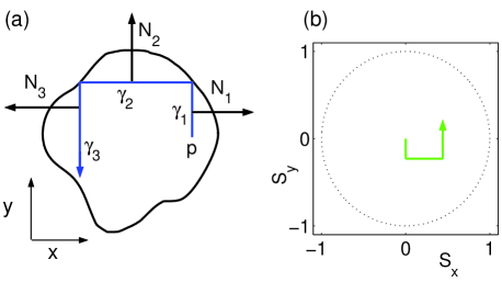
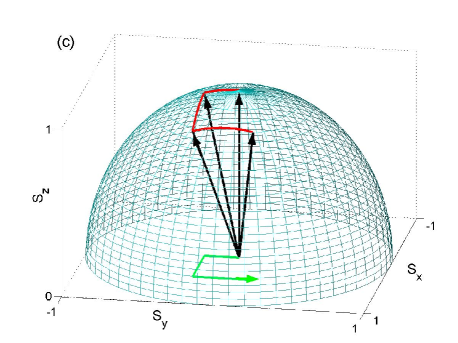
Figure 1: (Color online) (a) Electron motion inside a quantum dot. The trajectory consists of three straight segments $\gamma_{1}$, $\gamma_{2}$, and $\gamma_{3}$. (b) The corresponding spin evolution on the $s_{x}s_{y}$ plane, which is projected from (c). (c) The spin evolution induced by the Rashba spin-orbit interaction on the 3-dimensional unit sphere.

As an example of spin evolution induced by the Rashba interaction, let us consider an electron confined inside a quantum dot in Fig. 1(a), moving along the trajectory $\gamma$ which consists of three straight segments $\gamma_{1}$, $\gamma_{2}$, and $\gamma_{3}$ with the respective lengths $l_{1}$, $l_{2}$, $l_{3}$ and the angles $w_{1}=\pi/2$, $w_{2}=\pi$, $w_{3}=3\pi/2$. The initial spin state of this electron is polarized in $z$-direction, which is represented by an arrow in Fig. 1(c). This arrow is projected down to the origin $(0,0)$ on the $s_{x}s_{y}$ plane in Fig. 1(b). When the electron starts its motion from the initial point $p$ along the segment $\gamma_{1}$ (Fig. 1(a)), its spin rotates around the axis $\mathbf{N}_{1}=(1,0,0)$ and circumscribes an arc on the 3-dimensional sphere in Fig. 1(c). This curve is projected down onto a straight line on the $s_{x}s_{y}$ plane. This line is parallel to $\gamma_{1}$, but runs in a direction opposite to $\gamma_{1}$, as shown in Fig. 1(b). After the first collision with the boundary the electron further moves along the segment $\gamma_{2}$, while its spin rotates around $\mathbf{N}_{2}=(0,1,0)$ and circumscribes the second arc on the sphere in Fig. 1(c). The spin projection in Fig. 1(b) now runs parallel to $\gamma_{2}$ in the direction opposite to electron motion along $\gamma_{2}$. It is easy to see that the spin evolution on other segments follows the same rule: When an electron passes through the $j$-th segment in a certain direction, the spin circumscribes on the 3D unit sphere an arc around the axis $\mathbf{N}_{j}$. This arc, in its turn, is projected onto the $s_{x}s_{y}$ plane as a straight line parallel to the electron trajectory, but oppositely directed to it.

Further, let us proceed from the spin evolution on individual trajectories to the spin evolution averaged over an ensemble of trajectories. We consider an ensemble of electrons distributed uniformly within a bounded area of a 2-dimensional heterostructure. At $t=0$ these electrons have random outgoing angles but the same spins polarized in $z$-direction. Let $s_{z}^{(i)}(t)$ be the $z$ component of the electron spin at time $t$ for the $i$-th trajectory. Then, in our numerical simulations the integral in Eq. (20) can be replaced by the sum,

$$P^{z}_{c}(t)=\frac{1}{n}\sum_{i=1}^{n}s_{z}^{(i)}(t),$$ (33)

where the sum runs over $n$ individual trajectories. The so averaged spin polarization will be calculated in the following five systems:

(a)

In 2-dimensional bulk (Fig. 2(a)) with the elastic collision length $l$ distributed according to the Poisson law Prob$(l)=e^{-l/l_{m}}/l_{m}$, where $l_{m}$ is the mean free path. It is a stochastic open system. This is just the system where the conventional D’yakonov-Perel’ spin relaxation has to be observed.

(b)

In a ballistic circular quantum dot of radius $1$ with the smooth boundary in Fig. 2(b). Since the boundary is smooth, the incident and reflection angles on the boundary are the same. Since the system is ballistic, no scattering occurs inside the dot. It is an integrable system with a high spatial symmetry.

(c)

In a ballistic triangular quantum dot with the smooth boundary in Fig. 2(c). It is an integrable system of lower symmetry compared to the circular dot.

(d)

In a generalized Sinai billiard with the smooth boundary in Fig. 2(d). It is a deterministic but strongly chaotic system. The boundary geometry generates an ergodic dynamics in the phase space.

(e)

In a ballistic circular quantum dot like Fig. 2(b), but with random reflections from the boundary. The reflection angle takes random values between $-\pi/2$ and $\pi/2$ with respect to the boundary normal. It is a stochastic closed system and corresponds to a quantum dot whose boundary is not perfect in the scale of the electron Fermi wavelength.

The mean free path $l_{m}$ in bulk in Fig. 2(a) is set to $1$. The sizes of the triangular and Sinai dots, as shown in Fig. 2(c) and (d), are chosen to be $\sqrt{2\pi}\approx 2.5066$ and $\sqrt{32\pi/(16-\pi)}\approx 2.7961$, such that these dots have the same area $\pi$ as that of the circular dot in Fig. 2(b). We will use the dimensionless time unit, such that during the time interval 1 a particle moving with the Fermi velocity travels a distance of the length 1.

Figure 2: (Color online) Electrons trajectories (solid lines) for short time intervals: (a) in bulk, (b) circular quantum dot, (c) triangular quantum dot, and (d) Sinai quantum dot.

III.2 III.2 Results of the numerical simulations

In Fig. 3 the time dependences of $P^{z}_{c}(t)$ for $2124$ electrons in the open system (Fig. 2(a)) with $L_{so}=10$, $6$ and $2$ are plotted by solid curves $C_{1}$, $C_{2}$, and $C_{3}$. One can see that the relaxation time increases with $L_{so}$. These curves can be fitted by the well known expression for the longitudinal DP relaxation Ivchenko ,

$$P_{\tiny\mbox{DP}}(t)=\exp\left(\frac{-4\,t\,l_{m}}{L_{so}^{2}}\right),$$ (34)

which is shown by the dashed curves in Fig. 3. This expression was derived under the assumption of sufficiently large $L_{so}\gg l_{m}$. For not so large $L_{so}$ the fitting is not good, as it can be seen for the curve $C_{3}$ around its first drop at $t=4$. In this regime the spin rotates rather fast, so that most of the spins $s_{z}^{(i)}(t)$ evolve to negative values before the electrons encounter their first collisions with impurities. Therefore, $P^{z}_{c}(t)$ can evolve to a deep negative value within a short time interval. But later on $P^{z}_{c}(t)$ approaches to the asymptotic value $P^{z}_{c}=0$ (curve $C_{3}$ in Fig. 3). These results from Monte Carlo simulations confirm the well known DP relaxation in unbounded systems.

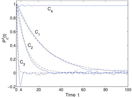
Figure 3: Solid curves $C_{1}$, $C_{2}$, and $C_{3}$ represent the time dependent polarization $P^{z}_{c}(t)$ for $2124$ particles in an unbounded QW with $L_{so}=10$, $6$, $2$ and the mean free path $l_{m}=1$. The particles were initially placed inside a circular area of the radius $R=1$ and polarized in $z$-direction. The dashed curves depict the DP relaxation calculated from Eq. (34). For comparison, curve $C_{4}$ shows $P^{z}_{c}(t)$ for $2124$ particles confined inside a circular dot of the radius $R=1$ and $L_{so}=10$.

If electrons are confined inside the smooth circular dot (Fig. 2(b)), the relaxation of $P^{z}_{c}(t)$ is considerably suppressed, so that at large $L_{so}$ the spin polarization remains close to $1$ at large times, as the curve $C_{4}$ in Fig. 3 demonstrates for the case of $L_{so}=10$. At this regime, the suppression of relaxation takes place in all other quantum dots, like the circular dot with the rough boundary (curve $C_{6}$), the triangular dot (curve $C_{7}$), and the Sinai billiard (curve $C_{8}$) in Fig. 4. In all of these curves the $P^{z}_{c}(t)$ values fall into the range between $0.97$ and $0.98$ at large times up to $t=10^{3}$.

On the other hand, the spin polarization evolves very fast down to $0$ if $L_{so}$ is smaller than the dot size. The corresponding time dependence of $P^{z}_{c}(t)$ is similar to that shown in Fig. 3 (curve C₃), with a sharp drop at the beginning followed by oscillations around zero.

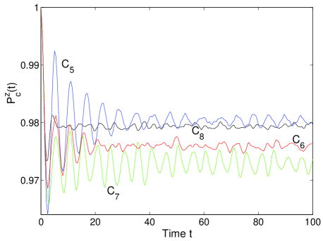
Figure 4: (Color online) Time dependence of $P^{z}_{c}(t)$ for $L_{so}=10$ in the smooth circular dot (curve $C_{5}$), the circular dot with the rough boundary (curve $C_{6}$), the triangular dot (curve $C_{7}$), and the Sinai billiard (curve $C_{8}$).

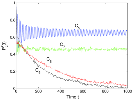
Figure 5: (Color online) Time dependence of $P^{z}_{c}(t)$ for $L_{so}=2$ in the smooth circular dot (curve $C_{5}$), the circular dot with the rough boundary (curve $C_{6}$), the triangular dot (curve $C_{7}$), and the Sinai billiard (curve $C_{8}$).

For an intermediate $L_{so}$ the spin relaxes according to different scenarios, depending on the quantum dot geometry. As an example, Fig. 5 shows the function $P^{z}_{c}(t)$ for various dot geometries at $L_{so}=2$. After a fast initial drop, the polarization further relaxes to 0 in the Sinai billiard (curve $C_{8}$) and in the circular dot with the rough boundary (curve $C_{6}$). However, in the smooth circular (curve $C_{5}$) and triangular (curve $C_{7}$) dots this function oscillates around a constant value at large times. It should be noted that in the former two examples the spin polarization relaxes to zero at much longer times than the DP relaxation time in the unbounded system (Fig. 3), although the mean elastic scattering length there is comparable to the dot size. The relaxation times for $C_{6}$ and $C_{8}$ in Fig. 5 increase rapidly with higher $L_{so}$. Thus, at $L_{so}=10$ we could not detect any systematic decrease of the spin polarization in the Sinai billiard and rough circular dot, up to $t=10^{3}$, which is by an order of magnitude larger than the range plotted in Fig. 4.

An interesting feature of $P^{z}_{c}(t)$ in the regular systems, like the triangular and smooth circular dots, is the apparent oscillation of the polarization. It can be seen at Figs. 4 and 5, although the oscillations in the latter figure are more profound for the case of the circular dot, compared to almost vanishing ripples in the triangle. These oscillations do not disappear at large times and their amplitude increase with the strength of SOI. We can not say much about their nature. Probably, they are associated with the role of periodic trajectories in regular systems. A special study is required to understand the origin and characteristics of these oscillations.

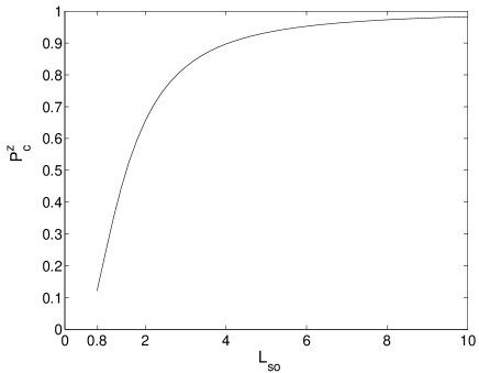
Figure 6: The residual polarization $P^{z}_{c}$ vs the spin rotation length $L_{so}$ for a smooth circular dot.

At long time the spin polarizations in both regular quantum dots (triangle and smooth circle) in Fig. 4 and 5 oscillate around certain nonzero residual values. These residual polarizations $P^{z}_{c}$ are $L_{so}$ dependent, as plotted in Fig. 6 for the circular dot.

III.3 III.3 Spin evolution along individual trajectories

The existence of the nonzero residual polarization in regular quantum dots and long spin relaxation time in chaotic systems are fundamentally distinct from the DP spin relaxation in the boundless QW. Such a distinction is surprising, because at first sight the spin walks on the sphere in Fig. 1(c) should be randomized by scattering of particles from dot boundaries, similar to randomization by impurity scattering in unbounded systems. However, this simple point of view is wrong, because there is an important difference between the impurity scattering and the boundary scattering. For convenience, let us define the scattering with a direction change smaller than $\pi/2$ as a ’forward’ scattering and that larger than $\pi/2$ as a ’backward’ scattering. If the particles are isotropically scattered by an impurity, half of them continue to move ’forward’. However, if the particles are scattered by a smooth boundary, the particles with incident angles between $-\pi/4$ to $\pi/4$ with respect to the boundary normal will be reflected ’backward’. Since statistically more particles hit the boundary within this range of angles, the ’backward’ scattering prevails in DQ’s. This property of particle scattering can also be extended to QD’s with rough boundaries. Further, according to Fig. 1, a ’backward’ particle motion is mapped onto a ’backward’ spin walk. Hence, if the spin moves away from the north pole in Fig. 1, after a boundary scattering the spin is more likely bounced back towards the north pole. Such a non-Markovian statistics of the spin walks gives a clue for understanding the numerical results in subsection III.2.

In order to make this argument more clear it is instructive to study in detail the spin evolution along a single trajectory. As described in Fig. 1, the spin motion on the unit sphere can be projected onto the $s_{x}s_{y}$ plane. After a long time the spin path on the sphere will cover a region and produce a certain pattern on the $s_{x}s_{y}$ plane. In the circular dot this pattern looks rather ordered. If the electron moves along a triangular periodic trajectory (Fig. 7(a)), the pattern is a rounded triangle (Fig. 7(i)). If the trajectories are hexahedral and star-like (Fig. 7(b) and (c)), the corresponding patterns are a rounded hexagon and a rounded star (Fig. 7(j) and (k)). If the trajectories are non-periodic, e.g., Fig. 7(d), the pattern is a disc (Fig. 7(l)). A common feature of these patterns is that they have the same size, which is less than $1$ in the case of $L_{so}=5$. These patterns are highly stable up to the observation time $t=10^{4}$. It implies that the spin on the unit sphere cannot move far away from the north pole, so that $s_{z}^{(i)}(t)$ cannot take negative values. Our analysis of various trajectories with various initial conditions has confirmed this general feature of the spin evolution in the circular dot. Hence, a non-zero $P^{z}_{c}$ in Fig. 6 at infinitely long time is obviously expected.

In the triangular dot, two periodic and one non-periodic trajectories are shown in Fig. 7(f), (g), and (h). The corresponding spin patterns (Fig. 7(n), (o), and (p)) are less symmetric and have less predictable sizes than those in the circular dot. For the trajectory in Fig. 7(g) the pattern in Fig. 7(o) touches the circular border. Nevertheless, our investigation shows that the patterns of most other trajectories are quite stable up to the observation time 10⁴ and do not touch the boarder. On this reason the spin polarization being averaged over trajectories is expected to relax to a positive residual value, although this value is smaller than that in the smooth circular dot.

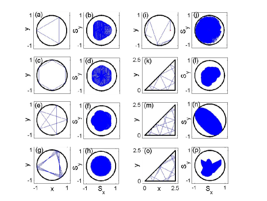
Figure 7: Electron trajectories on the $xy$ plane ((a)-(h)) and respective spin evolution patterns on the $s_{x}s_{y}$ plane ((i)-(p)) for $L_{so}=5$. (a), (b), and (c) Periodic triangular, hexahedral, and star-like trajectories in the smooth circular dot. (d) A non-periodic trajectory in the smooth circular dot. (e) A stochastic trajectory in the rough circular dot. (f) and (g) Two periodic trajectories in the triangular dot. (h) A non-periodic trajectory in the triangular dot.

In the circular dot with a rough boundary, the reflection angles are stochastic, as shown in Fig. 7(e). Within the observation time $t=10^{3}$ the corresponding spin pattern on the $s_{x}s_{y}$ plane has spread out to a much larger area (Fig. 7(m)) than those in the smooth circular dot (Fig. 7(i)-(l)). Furthermore, the pattern in (Fig. 7(m)) is still expanding. The corresponding spin state on the 3D sphere can penetrate into the lower hemisphere after $t=10^{3}$. However, it can return back to the north sphere again. Therefore, the $z$ component of this spin state oscillates between negative and positive values. When averaged over many trajectories, such oscillations sum up to a relaxation curve, similar to $C_{6}$ in Fig. 5.

In the Sinai billiard, the $s_{x}s_{y}$ pattern resembles that in the rough circular dot. Consequently, the spin relaxation dynamics in both cases have similar characteristics (curves $C_{6}$ and $C_{8}$ in Fig. 5).

A general trend seen from Fig. 7 is that the confinement of the particle motion in QD’s makes the spin to be also confined within the upper hemisphere, if $L_{so}$ is larger than the size of the QD’s. For a smooth circular dot, this trend can be easily understood from the ’backward’ scattering effect described at the beginning of this subsection. Since all trajectories in this case have a simple geometry, one can easily see that particles are more frequently scattered from the boundary in a ’backward’ direction. But although this argument holds for general bounded systems, it is less evident for other QD’s besides the smooth circular dot. In general case, the trend toward the spin confinement can be argued in a different way: As seen from Fig. 1, the projected spin path on the $s_{x}s_{y}$ plane in Fig. 1(b) is more or less a rescaled curve of its particle trajectory in Fig. 1(a). But in reality the mapping from a trajectory to the corresponding spin path is not simply a rescaling, because the spin rotations on the sphere are non-commutative. For example, a closed particle trajectory is in general mapped onto an open spin path. However, if $L_{so}$ is large, the spin path is restricted to a small part of the sphere. According to Eq. (21-22), a closed particle trajectory produces an open spin path of the linear size $\sim 1/L_{so}$, while the distance between the initial and the end points of the path is only $\sim 1/L_{so}^{2}$. The mapping between the trajectories and the spin paths is then similar to a mapping between two Euclidean spaces. Therefore, with the accuracy $1/L_{so}^{2}$, the spin paths are the rescaled particle trajectories and those paths are confined because the particle trajectories are confined. It should be noted that such a tendency for the spin confinement turns out to be strong even for not so large $L_{so}$, as one can see from the spin dynamics shown in Fig. 5 for $L_{so}=2$.

The above argument about the spin confinement does not take into account a long time evolution. Even at large $L_{so}$, small corrections due to non-commutativity of spin walks will accumulate in time. As a result, the spin can slowly drift toward the lower hemisphere. The expanding pattern in Fig. 7(m) of the rough circular dot is an example of such a long time behavior. However, in contrast to that unstable pattern, the patterns from regular systems (Fig. 7(i)-(p) besides (m)) remain stable in time. This difference between the single trajectories of random and regular systems is consistent with the spin relaxation curves shown in Fig. 5.

Such a distinction between regular and chaotic systems follows from fundamental properties of regular and chaotic systems. It can be understood from consideration of periodic orbits. After a particle runs along a periodic orbit $\gamma$ and completes a period, its initial spin state $\chi$ will evolve to $U_{\gamma}\chi$ with $U_{\gamma}=\exp[-i\Omega\mathbf{R}\bm{\sigma}]$, which represents a rotation around the axis $\mathbf{R}$ through the angle $2\Omega$. Both $\mathbf{R}$ and $\Omega$ are determined entirely by the geometry of $\gamma$ and by the value of $L_{so}$. After the particle repeats $w$ periods, all spin positions $(U_{\gamma})^{w}\chi$, corresponding to the end points of all periods $w=1,2,\cdots$, are located on a closed circle. This circle can be obtained by rotating the north pole around $\mathbf{R}$, if the initial $\chi$ is related to the spin polarized in the north pole direction. The other points on the periodic orbit are mapped onto spin states around this circle. Taking many periodic orbits into account, one obtains a set of different axes $\mathbf{R}$ and consequently a set of circles passing through the north pole. Hence, when averaged over all periodic orbits, spin spends more time in the upper hemisphere. This means that at least the family of the periodic orbits contributes to a nonzero residual polarization. How significant is this contribution to the whole residual value depends on the amount of the periodic orbits in a system, which is quite different in regular and chaotic systems. In a regular system the family of periodic orbits has a finitely positive measure and a bundle of adjacent nearly periodic orbits. These adjacent trajectories behave like periodic orbits if the time is not too large, because their linear deviation in time from the periodic orbits is small. On the contrary, the periodic orbits in chaotic systems are of zero measure Gutzwiller . Furthermore, their adjacent trajectories deviate from them exponentially fast. Therefore, with increasing time, the weight of the periodic orbits and their adjacent trajectories becomes exponentially small in chaotic systems, while it is a nonzero value in regular systems. Hence, as long as we consider only periodic orbits, the residual spin polarization has to be a positive number for regular systems and zero for chaotic systems.

The individual trajectory study in a larger time scale carried out in this subsection helps us to understand some of the results in subsection III. 2. However, although the existence of the nonzero residual polarization $P^{z}_{c}$ is apparent from Figs. 3-6, one cannot exclude a possibility that $P^{z}_{c}$ will decay to zero in a much larger time scale, since the numerical simulations in all these figures are truncated within a finite time. Therefore, we can not definitely answer the question whether the spin polarization relaxes to zero at the infinitely long time, or to a nonzero residual value. For the smooth circular dot the latter alternative is corroborated by an analysis of the spin polarization from the exact solution of the Schrödinger equation, as shown in the next section.

IV IV Quantum mechanical polarization in the circular quantum dot

Due to the time reversal symmetry, the quantized energy levels $E_{n}$ of the Hamiltonian $H$ in Eq. (1) are, at least, two fold degenerate with the corresponding spinor eigenfunctions $\varphi_{n\mathrm{a}}$, where $\mathrm{a}\in\{\pm\}$ is the degeneracy index. In the basis of these states a normalized wave function $\psi(\mathbf{r},t)$ can be expanded as

$$\psi(\mathbf{r},t)=\sum_{n\mathrm{a}}c_{n\mathrm{a}}\varphi_{n\mathrm{a}}(\mathbf{r})\,e^{-i\,E_{n}t/\hbar}\,,$$ (35)

with the coefficient

$$c_{n\mathrm{a}}=\int\varphi_{n\mathrm{a}}^{{\dagger}}(\mathbf{r})\psi(\mathbf{r})\,d^{\,2}r\,.$$ (36)

The expression of $\psi(\mathbf{r},t)$ in Eq. (35) differs from Eq. (3) only by the degeneracy index $\mathrm{a}$, which is explicitly written here for convenience of our further analysis. Taking the notation

$$\psi_{n\mathrm{a}}(\mathbf{r},t)=c_{n\mathrm{a}}\varphi_{n\mathrm{a}}(\mathbf{r})\,e^{-i\,E_{n}t/\hbar},$$ (37)

and $\psi_{n\mathrm{a}}(\mathbf{r})=\psi_{n\mathrm{a}}(\mathbf{r},0)$, the $z$ component of the quantum mechanical polarization in Eq. (5) can be expressed as

$$P^{z}(t) = \langle\psi(\mathbf{r},t)|\sigma^{z}|\psi(\mathbf{r},t)\rangle$$

$$= \sum_{n\mathrm{a}\mathrm{b}}\int\psi_{n\mathrm{a}}^{\dagger}(\mathbf{r})\sigma^{z}\psi_{n\mathrm{b}}(\mathbf{r})\,d^{\,2}r$$

$$+\!\!\!\!\!\sum_{n\neq m,\mathrm{a}\mathrm{b}}\!\int\psi_{n\mathrm{a}}^{\dagger}(\mathbf{r})\sigma^{z}\psi_{m\mathrm{b}}(\mathbf{r})\,e^{i(E_{n}-E_{m})t/\hbar}\,d^{\,2}r.$$

The first sum in this equation is time independent, while the second sum oscillates in time, so that its average over a sufficiently long time interval turns to zero. It is interesting to find out whether the former term coincides with the residual polarization in Fig. 6. Such a coincidence is not evident because the time dependent sum can give rise to large variations of $P^{z}(t)$ after long time $t$. Moreover, the semiclassical theory employed in the previous section can be not valid for times larger than the mean distance between energy levels near the Fermi energy. We can check such a coincidence at least for the simple case of a circular dot with the smooth boundary, by calculating the residual polarization

$$P^{z}=\sum_{n\mathrm{a}\mathrm{a^{\prime}}}\int\psi_{n\mathrm{a}}^{\dagger}(\mathbf{r})\sigma^{z}\psi_{n\mathrm{a^{\prime}}}(\mathbf{r})\,d^{\,2}r,$$ (39)

because the analytic solution of the Schrödinger equation with the arbitrarily strong Rashba interaction is available Tsitsishvili . In this section only the key steps of the calculation are presented, while the calculation in detail is shown in the Appendix.

Let us consider a circular quantum dot of radius $R$ with the confining potential

$$V(\rho)=\left\{\begin{array}[]{ll}0&\mbox{ for }0\leq\rho\leq R\\ \infty&\mbox{ for }R>\rho\end{array}\right.,$$ (40)

written as a function of the polar coordinates $\mathbf{r}=\mathbf{r}(\rho,\phi)$. The eigenfunctions of the n-th eigenvalue $E_{n}$ are Tsitsishvili

$$\varphi_{n+}(\mathbf{r})=\left(\begin{array}[]{c}e^{i\nu\phi}f_{\nu}(\rho)\\ e^{i(\nu+1)\phi}g_{\nu+1}(\rho)\end{array}\right)$$ (41)

and

$$\varphi_{n-}(\mathbf{r})=\left(\begin{array}[]{c}e^{-i(\nu+1)\phi}g^{*}_{\nu+1}(\rho)\\ -e^{-i\nu\phi}f^{*}_{\nu}(\rho)\end{array}\right),$$ (42)

where the function

$$\left(\begin{array}[]{c}f_{\nu}(\xi)\\ g_{\nu}(\xi)\end{array}\right)=d\left(\begin{array}[]{c}-a_{\nu}J_{\nu}(k_{+}\xi)+J_{\nu}(k_{-}\xi)\\ a_{\nu-1}J_{\nu}(k_{+}\xi)+J_{\nu}(k_{-}\xi)\end{array}\right),$$ (43)

contains the $\nu$-th order Bessel functions of the first kind $J_{\nu}(\xi)$, the normalization constant $d$, the parameters

$$a_{\nu}=\frac{J_{\nu}(k_{-})}{J_{\nu}(k_{+})}=-\frac{J_{\nu+1}(k_{-})}{J_{\nu+1}(k_{+})},$$ (44)

the wave numbers

$$k_{\pm}=\frac{\sqrt{b^{\,2}+4\varepsilon}\mp b}{2},$$ (45)

and the index

$$\nu=\lambda-3/2\hskip 8.5359pt\mbox{ with }\hskip 8.5359pt\lambda=1,\,2,\,\cdots.$$ (46)

Therein, the dimensionless parameters $\xi=\rho/R$, $\varepsilon=2m^{*}ER^{2}/\hbar^{2}$, and $b=2\alpha_{R}m^{*}R/\hbar^{2}$ have been used. The wave numbers $k_{\pm}$ are quantized because the energy levels $\varepsilon$ are determined by the zeros of the function

$$Z_{\nu}(\varepsilon):=J_{\nu}(k_{-})J_{\nu+1}(k_{+})+J_{\nu}(k_{+})J_{\nu+1}(k_{-}).$$ (47)

We chose the plane wave

$$\psi(\mathbf{r})=\left(\begin{array}[]{c}1\\ 0\end{array}\right)e^{i\mathbf{k}\mathbf{r}}$$ (48)

as the initial state. After inserting $\varphi_{n+}(\mathbf{r})$ from Eq. (41) and $\varphi_{n-}(\mathbf{r})$ from Eq. (42) together with Eq. (37) into Eq. (39) and averaging over directions of the vector $\mathbf{k}$ we obtain

$$P^{z}=2\pi\sum_{n}\left(|c_{n+}|^{2}-|c_{n-}|^{2}\right)(F_{n}-G_{n}),$$ (49)

with

$$F_{n}=d^{\,2}\left[\,a_{\nu}^{2}\,I_{\nu}^{(1)}-2a_{\nu}\,I_{\nu}^{(2)}+I_{\nu}^{(3)}\right]$$

$$G_{n}=d^{\,2}\left[\,a_{\nu}^{2}\,I_{\nu+1}^{(1)}+2a_{\nu}\,I_{\nu+1}^{(2)}+I_{\nu+1}^{(3)}\right],$$ (50)

where the coefficients $I_{\nu}^{(1)}$, $I_{\nu}^{(2)}$, and $I_{\nu}^{(3)}$ are presented in Eq. (74). The coefficients $|c_{n\pm}|^{2}$ in Eq. (49) can be written as

$$|c_{n+}|^{2}=4\pi^{2}\,d^{\,2}\,\left(\,-a_{\nu}\,I_{\nu}^{(4)}+I_{\nu}^{(5)}\,\right)^{2}$$

$$|c_{n-}|^{2}=4\pi^{2}\,d^{\,2}\,\left(\;a_{\nu}\,I_{\nu+1}^{(4)}+I_{\nu+1}^{(5)}\,\right)^{2},$$ (51)

with the coefficients $I_{\nu}^{(4)}$ and $I_{\nu}^{(5)}$ given by Eq. (LABEL:eq66). Using the dimensionless units, one has the radius $R=1$, the coupling constant $b=2/L_{so}$, and the wave number $k=2\pi R/\lambda$, where $\lambda$ is the electron wavelength. Hence the semiclassical range of parameters corresponds to $k\gg 1$.

The residual polarization calculated from Eq. (49) is shown in Fig. 8. The $P^{z}$ curves for $k=20$, $30$, and $40$ are very close to each other and merge into the dashed curve. This curve coincides with the residual polarization obtained from the semiclassical simulations in the previous section (Fig. 6). For $k=5$, $1$, and $0.1$, the curves are plotted in the dotted, solid, and dash-dotted curves, respectively. All the curves, as expected, have the common asymptotic value $1$ in the case of the weak spin-orbit coupling $L_{so}\rightarrow\infty$. In the opposite limit, $L_{so}\rightarrow 0$, the behavior of $P^{z}$ is nonanalytic and not much revealing. The strong oscillations in this limit increase with smaller wave numbers and signal about the appearance of large quantum beats in $P^{z}(t)$. This regime of $L_{so}$ is not interesting from the practical point of view because it implies unphysically large values of $\alpha_{R}$ for the typical dot radius $R=500nm$. In the practically important regime of $L_{so}\geq 1$ we note an apparent dependence of $P^{z}$ on $k$ at $k\leq 5$. This is a quantum effect which is not observed in our semiclassical simulations. In semiclassics the particle velocity determines the speed with which $P^{z}(t)$ approaches to the residual value $P^{z}$, but not this value itself.

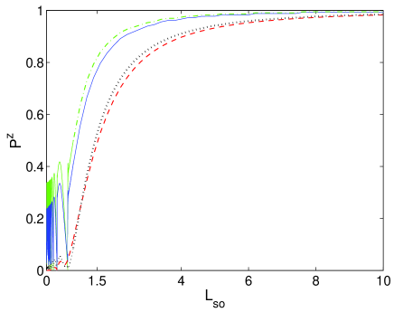
Figure 8: (Color online) The residual spin polarization $P^{z}$ vs $L_{so}$ with $k=20$, $30$, $40$, (dashed), $k=5$ (dotted), $k=1$ (solid), and $k=0.1$ (dash-dotted). The dashed curve coincides with the curve from Fig. 6.

V V Discussion

Summarizing the above results of the semiclassical Monte Carlo simulations and quantum mechanical calculations we can draw the following picture of the spin evolution in semiclassical quantum dots. In the dots with regular classical dynamics the spin polarization does not decay to zero at long time and its residual value coincides with the quantum mechanical spin polarization averaged over an infinitely long time interval. At least, we were able to check such a coincidence for the circular dot. On the other hand, in dots with chaotic or random dynamics the spin polarization relaxes to zero with the relaxation time much larger than the DP relaxation time in unbounded quantum wells. Such a decay down to zero can not be understood from the general quantum mechanical expression in Eq. (IV), because it implies that the average of $P^{z}(t)$ over an asymptotically long time interval is zero. However, Eq. (IV) predicts that this average is given by the first term in Eq. (IV), which is nonzero in general. Obviously, this contradiction is associated with quantum mechanical effects, which indicates that the semiclassical approximation is insufficient for analysis of the long time polarization evolution. In disordered mesoscopic systems the statistics of their energy spectrum together with quantum interference effects give rise to the so called quantum dynamical echo Prigodin which can contribute to the spin evolution at large times. This problem needs further study.

The predicted spin evolution can be measured experimentally. For an InAs dot doped up to 10¹¹cm^-2, the time unit in Figs. 3-5 is about 1 ps if the dot size is $L=0.5\mu m$. Hence, the spin polarization saturates to its residual value during first 20 ps and for $L_{so}=1\mu m$ the difference in the long time evolution between chaotic and regular dots can be observed in the nanosecond range. In order to suppress all inelastic spin relaxation mechanisms Khaetskii ; Woods ; Merkulov ; Semenov , the measurement must be done at sufficiently low temperatures. The Rashba spin-orbit interaction can be strong in InAs based heterostructures, with $L_{so}$ down to several hundreds nm. Moreover, it can be tuned in a wide interval by varying the gate voltage Nitta .

In conclusion, we performed path integral semiclassical simulations of spin evolution controlled by the Rashba spin-orbit interaction in quantum dots of various shapes. Our calculations revealed that the spin polarization dynamics in QD’s is quite different from the D’yakonov-Perel’ spin relaxation in bulk 2D systems. Such a distinction is not expected from the simple picture of the spin random walk, in particular when the rate of electron elastic scattering on impurities in bulk is equal to the mean frequency of electron scattering from the dot boundaries. We have also found an important distinction between long time spin evolutions in classically chaotic and regular systems. In the former case the spin polarization relaxes to zero within relaxation time much larger than the DP relaxation, while in the latter case it evolves to a time independent residual value. This value decreases with the stronger spin orbit interaction. We also analyzed the general quantum mechanical expression for the time dependent spin polarization. Using the exact solutions of the Schrödinger equation with Rashba SOI for a circular dot, we calculated the average of the spin polarization over an infinitely long time interval and compared the result with the residual polarization from the Monte Carlo simulations. We found that the residual values from these two approaches coincide, which confirms the results from the semiclassical simulations. On this basis, we conjecture that the nonzero residual value is a general property of regular systems. On the other hand, the spin relaxation down to zero in the Sinai billiard and circular dot with the rough boundary contradicts to what have to be expected from quantum mechanics. The long time memory due to the mesoscopic spin echo is assumed to be responsible for this contradiction.

VI Appendix

This appendix demonstrates a quantum mechanical calculation of the residual polarization $P^{z}$, as it is defined in Eq. (39). The calculation of the exact eigenfunctions of the Hamiltonian in Eq. (1) for the circular quantum dot can be found in Ref. Tsitsishvili , which is summarized in the following Eqs. (VI-VI).

In order to calculate the residual polarization (39), the wave function $\psi_{na}(\mathbf{r})$ is expanded in the basis of the eigenfunctions given by Eqs. (41-42). We note that for a symmetric presentation, the functions $f_{\nu}$ and $g_{\nu}$ have different definitions from those in Ref. Tsitsishvili . Inserting Eqs. (41-42) into the corresponding Schrödinger equation we obtain the equation for $f_{\nu}$ and $g_{\nu}$ in terms of the dimensionless parameters $\xi,\varepsilon$, and $b$ defined in the previous section,

$$[\triangle_{\nu}+\varepsilon]\,f_{\nu}(\xi)-b\,\nabla_{-(\nu+1)}\,g_{\nu+1}(\xi)=0,$$

$$[\triangle_{\nu+1}+\varepsilon]\,g_{\nu+1}(\xi)-b\,\nabla_{+\nu}\,f_{\nu}(\xi)=0,$$ (52)

with the Laplacian

$$\triangle_{\nu}=\frac{1}{\xi}\frac{d}{d\xi}\left(\xi\frac{d}{d\xi}\right)-\frac{\nu^{2}}{\xi^{2}}$$ (53)

and the nabla operator

$$\nabla_{\pm\nu}=\pm\left(\frac{d}{d\xi}\right)-\frac{\nu}{\xi}.$$ (54)

The solutions $(f_{\nu}(\xi),g_{\nu}(\xi))$ of these equations are

$$\left(\begin{array}[]{c}f_{\nu}(\xi)\\ g_{\nu}(\xi)\end{array}\right)=d\left(\begin{array}[]{c}-a_{\nu}J_{\nu}(k_{+}\xi)+J_{\nu}(k_{-}\xi)\\ a_{\nu-1}J_{\nu}(k_{+}\xi)+J_{\nu}(k_{-}\xi)\end{array}\right),$$ (55)

with the normalization constant $d$, the factors $a_{\nu}$ given by Eq. (44), and the wave vectors $k_{\pm}$ from Eq. (45). These wave vectors obey the relations

$$k_{+}k_{-}=\varepsilon,\hskip 8.5359ptk_{+}-k_{-}=-b,$$

$$\mbox{and }k_{+}+k_{-}=\sqrt{b^{2}+4\varepsilon}.$$ (56)

The quantized dimensionless energies $\varepsilon$ are determined by the zeros of the function in Eq. (47). This function stems from the determinant of the equation system in Eq. (VI) with the boundary conditions $f_{\nu}(\xi)=g_{\nu}(\xi)=0$ at $\xi=1$. Given a coupling constant $b$, the $n$-th quantized value $\varepsilon_{n}$ with $n=n(\lambda,\mu)$ is determined by the $\mu$-th zero of $Z_{\nu}(\varepsilon)$, where $\nu$ and $\lambda$ are related by Eq. (46). The allowed wave numbers $k_{\pm}$ are given by Eq. (45) with $\varepsilon=\varepsilon_{n}$. They correspond to the two degenerate eigenstates of the n-th energy level. The first root of the function $Z_{\nu}(\varepsilon)$ is zero for $\nu=1/2,3/2,...$ and is a positive value for $\nu=-1/2$ (see Fig. 9). The larger the value of $b$, the larger the second root of $Z_{\nu}(\varepsilon)$.

Figure 9: The function $Z_{\nu}(\varepsilon)$ for $\nu=-1/2$, $1/2$, and $3/2$. This function is singular at $\varepsilon=0$ for $\nu=-1/2$.

Substituting the wave functions in Eqs. (41-42) into Eq. (39) we obtain the residual polarization in the form

$$P^{z} = \sum_{n}\int_{0}^{1}\int_{0}^{2\pi}\left[\left(|c_{n+}|^{2}-|c_{n-}|^{2}\right)\left(f_{\nu}^{2}(\xi)-g_{\nu+1}^{2}(\xi)\right)\right.$$ (57)

$$+2c_{n+}^{*}c_{n-}f_{\nu}(\xi)g_{\nu+1}(\xi)e^{-i(2\nu+1)\phi}$$

$$\left.+2c_{n-}^{*}c_{n+}f_{\nu}(\xi)g_{\nu+1}(\xi)e^{i(2\nu+1)\phi}\right]\,d\phi\,\xi\,d\xi.$$

For the initial wave function given by Eq. (48), the constants $c_{n+}$ can be expressed as

$$c_{n+} = \int\left(\begin{array}[]{c}\varphi_{n+}^{(1)}(\mathbf{r})\\ \varphi_{n+}^{(2)}(\mathbf{r})\end{array}\right)^{\dagger}\,\left(\begin{array}[]{c}1\\ 0\end{array}\right)e^{i\mathbf{k}\mathbf{r}}\,d^{\,2}r$$

$$= \int\varphi_{n+}^{(1)\,*}(\mathbf{r})\,e^{i\mathbf{k}\mathbf{r}}\,d^{\,2}r$$

$$= \int_{0}^{2\pi}\int_{0}^{1}e^{i\left[k\xi\cos(\phi-\theta)-\nu\phi\right]}f_{\nu}(\xi)\xi\,d\xi\,d\phi,$$ (63)

where $\phi$ and $\theta$ stand for the angles of the vectors $\mathbf{r}$ and $\mathbf{k}$ with respect to the positive x-axis and $k=|\mathbf{k}|$. After the shift of the angular variable from $\phi-\theta$ to $\phi$ the above integral transforms to

$$c_{n+}=e^{-i\nu\theta}\int_{0}^{2\pi}\int_{0}^{1}e^{i\left[k\xi\cos(\phi)-\nu\phi\right]}f_{\nu}(\xi)\xi\,d\xi\,d\phi.$$ (64)

Substituting $t=\phi+\pi/2$ and $m=\nu$ into the integral representation of the Bessel function Gradshteyn ,

$$J_{m}(z)=\frac{1}{2\pi}\int_{-\pi}^{\pi}e^{i\,[z\sin(t)-mt]}\,dt,$$ (65)

we obtain

$$2\pi\,e^{i\nu\pi/2}J_{\nu}(z)=\int_{0}^{2\pi}e^{i\,[z\cos(\phi)-\nu\phi]d\phi}.$$ (66)

By using this identity, Eq. (64) can be written as

$$c_{n+} = 2\pi\,e^{i\nu(\pi/2-\theta)}\int_{0}^{1}J_{\nu}(k\xi)\,f_{\nu}(\xi)\xi\,d\xi.$$ (67)

By analogy, one has

$$c_{n-}=2\pi\,e^{i(\nu+1)(\pi/2-\theta)}\int_{0}^{1}J_{\nu+1}(k\xi)\,g_{\nu+1}(\xi)\xi\,d\xi.$$ (68)

After integrating Eq. (57) over $\phi$ and the direction $\theta$ of $\mathbf{k}$ (integration over $\theta$ is similar to that over $\theta_{\mathbf{k}}$ in Eq. (20)), the second and third terms in Eq. (57) vanish and only the first term remains. Introducing the parameters

$$F_{n}=\int_{0}^{1}f_{\nu}^{2}(\xi)\xi\,d\xi\hskip 8.5359pt\mbox{ and }\hskip 8.5359ptG_{n}=\int_{0}^{1}g_{\nu+1}^{2}(\xi)\xi\,d\xi,$$ (69)

the final expression for the residual polarization can be written as

$$P^{z}=\frac{\sum_{n}\left(|c_{n+}|^{2}-|c_{n-}|^{2}\right)(F_{n}-G_{n})}{\sum_{n}\left(|c_{n+}|^{2}+|c_{n-}|^{2}\right)(F_{n}+G_{n})}.$$ (70)

For numerical calculations we explicitly wrote the norm of the normalized wave function $\psi(\mathbf{r},t)$ in the denominator. In this form the expression in Eq. (70) is also valid for non-normalized wave functions, because the normalization constants $d$ in the numerator and denominator are canceled with each other.

The polarization $P^{z}$ in Eq. (70) is determined by the four integrals $c_{n\pm}$, $F_{n}$, and $G_{n}$. They can be calculated by using the formula Lebedev

$$\int_{0}^{\,l}\xi\,J_{\nu}(\lambda\,\xi)J_{\nu}(\kappa\,\xi)\,d\xi$$ (71)

$$\;\;\;\;=\frac{l\,[\kappa J_{\nu}(\lambda\,l)J_{\nu+1}(\kappa\,l)-\lambda J_{\nu}(\kappa\,l)J_{\nu+1}(\lambda\,l)]}{\kappa^{2}-\lambda^{2}}.$$

Consequently, the integrals in Eq. (69) can be written in the closed form

$$F_{n}=d^{\,2}\left[\,a_{\nu}^{2}\,I_{\nu}^{(1)}-2a_{\nu}\,I_{\nu}^{(2)}+I_{\nu}^{(3)}\right],$$ (72)

$$G_{n}=d^{\,2}\left[\,a_{\nu}^{2}\,I_{\nu+1}^{(1)}+2a_{\nu}\,I_{\nu+1}^{(2)}+I_{\nu+1}^{(3)}\right],$$ (73)

with

$$I_{\nu}^{(1)}=\frac{J_{\nu}(k_{+})^{2}+J_{\nu+1}(k_{+})^{2}}{2}-\frac{\nu J_{\nu}(k_{+})J_{\nu+1}(k_{+})}{k_{+}},$$

$$I_{\nu}^{(2)}=\frac{k_{-}J_{\nu}(k_{+})J_{\nu+1}(k_{-})-k_{+}J_{\nu}(k_{-})J_{\nu+1}(k_{+})}{k_{-}^{2}-k_{+}^{2}},$$

$$I_{\nu}^{(3)}=\frac{J_{\nu}(k_{-})^{2}+J_{\nu+1}(k_{-})^{2}}{2}-\frac{\nu J_{\nu}(k_{-})J_{\nu+1}(k_{-})}{k_{-}}.$$

(74)

By analogy, calculating the integrals in Eqs. (67-68) we obtain

$$|c_{n+}|^{2}=4\pi^{2}\,d^{\,2}\,\left(\,-a_{\nu}\,I_{\nu}^{(4)}+I_{\nu}^{(5)}\,\right)^{2},$$ (75)

$$|c_{n-}|^{2}=4\pi^{2}\,d^{\,2}\,\left(\;a_{\nu}\,I_{\nu+1}^{(4)}+I_{\nu+1}^{(5)}\,\right)^{2},$$ (76)

with

$$I_{\nu}^{(4)} = \frac{k_{+}J_{\nu}(k)J_{\nu+1}(k_{+})-kJ_{\nu}(k_{+})J_{\nu+1}(k)}{k_{+}^{2}-k^{2}},$$

$$I_{\nu}^{(5)} = \frac{k_{-}J_{\nu}(k)J_{\nu+1}(k_{-})-kJ_{\nu}(k_{-})J_{\nu+1}(k)}{k_{-}^{2}-k^{2}}.$$

For small $b$ the spin polarization approaches to $P^{z}=1$, as it must be in the absence of the spin-orbit interaction. It follows from the relation $k_{-}-k_{+}=b\approx 0$ in Eq. (VI), which results in $f_{\nu}(\xi)\approx 0$, according to the definition in Eq. (55). Hence, the two quantities $|c_{n+}|$ and $F_{n}$, which contain $f_{\nu}(\xi)$, vanish in $P^{z}$. Therefore, the sums in the numerator and denominator of $P^{z}$ become the same, which gives rise to $P^{z}=1$.

For large $b$, we have $P^{z}\rightarrow 0$, which is due to the large difference between $k_{+}$ and $k_{-}$, namely, $k_{-}-k_{+}=b\gg 1$. According to the asymptotic behavior Lebedev

$$J_{\nu}(x)=\sqrt{\frac{2}{\pi x}}\cos\left(x-\frac{\pi}{2}\left(\nu+\frac{1}{2}\right)\right)+O\left(\frac{1}{x}\right)$$ (78)

of the Bessel function at large $x$, the magnitude of the oscillating function $J_{\nu}(k_{+})$ is much larger than $J_{\nu}(k_{-})$ by the order of $\sqrt{k_{-}/k_{+}}$. Therefore, the leading terms of $I_{\nu}^{(4)}$ and $I_{\nu}^{(5)}$ in Eq. (LABEL:eq66) behave like

$$I_{\nu}^{(4)} \sim \frac{J_{\nu}(k_{+})J_{\nu+1}(k)}{k},$$

$$I_{\nu}^{(5)} \sim \frac{J_{\nu}(k)J_{\nu+1}(k_{-})}{k_{-}}.$$ (79)

The first term is much larger than the second one. Consequently, both $c_{n+}$ and $c_{n-}$ are dominated by $I_{\nu}^{(4)}$ and have the same limit for large $b$. By analogy, $F_{n}$ and $G_{n}$ also have the same limit. Therefore, both $|c_{n+}|^{2}-|c_{n-}|^{2}$ and $F_{n}-G_{n}$ in the numerator of Eq. (70) become small and hence $P^{z}=0$ for $b\rightarrow\infty$.

Acknowledgement: This work was supported by RFBR No. 03-02-17452 and the Swedish Royal Academy of Science; A.G.M. acknowledges the hospitality of NCTS in Taiwan. C.-H.C. acknowledges the hospitality of Lund university in Sweden and the Science Institute in the university of Iceland.

References

- (1) D. D. Awschalom, D. Loss, and N. Samarth, Semiconductor Spintronics and Quantum Computation, Springer-Verlag, Berlin (2002).
- (2) M. I. D’yakonov and V. I. Perel’, Fiz. Tverd. Tela, 13, 3581 (1971) [Sov. Phys. Solid State, 13, 3023 (1972)]; Zh. Eksp. Teor. Fiz. 60, 1954 (1971) [Sov. Phys. JETP 33, 1053 (1971)].
- (3) A. V. Khaetskii, Y. V. Nazarov, Phys. Rev. B 61, 12639 (2000); A. V. Khaetskii, Y. V. Nazarov, Phys. Rev. B 64, 125316 (2001).
- (4) L. M. Woods, T. L. Reinecke, Y. Lyanda-Geller, Phys. Rev. B 66, 161318 (2002).
- (5) I. A. Merkulov, A. I. Efros, M. Rosen, Phys. Rev. B 65, 205309 (2002).
- (6) Y. G. Semenov, K. W. Kim, Phys. Rev. Lett. 92, 026601 (2004).
- (7) J. Nitta et. al., Phys. Rev. Lett 78, 1335 (1997); D. Grundler, Phys. Rev. Lett 84, 6074 (2000).
- (8) Yu. L. Bychkov and E. I. Rashba, J. Phys. C 17, 6093 (1984).
- (9) G. Dresselhaus, Phys. Rev. 100, 580 (1955).
- (10) R. Eppenga, H. F. M. Schuurmans, Phys. Rev. B 37, 10923 (1988).
- (11) B. Jusserand, D. Richards, G. Allan, C. Priester, and B. Etienne, Phys. Rev. B 51, 4707 (1995).
- (12) L. S. Schulman, Techniques and Application of Path Integration (Wiley, N. Y. 1981).
- (13) E. L. Ivchenko, Superlattices and other heterostructures: symmetry and optical phenomena, Springer-Verlag, New York (1997).
- (14) M. C. Gutzwiller, Chaos in Classical and Quantum Mechanics (Springer, N.Y., 1990).
- (15) V.N. Prigodin, B. L. Altshuler, K.B. Efetov, S. Iida, Phys. Rev. Lett. 72, 546 (1994).
- (16) E. Tsitsishvili, G.S. Lozano, and A.O. Gogolin, cond-mat 0310024 v1, (2003).
- (17) I.S. Gradshteyn and I.M. Ryzhik, Table of Integrals, Series, and Products, Academic Press, London, (2000).
- (18) N.N. Lebedev, Special Functions, Dover Pubns, (1972).