Weak disorder expansion for localization lengths of quasi-1D systems

Abstract

A perturbative formula for the lowest Lyapunov exponent of an Anderson model on a strip is presented. It is expressed in terms of an energy dependent doubly stochastic matrix, the size of which is proportional to the strip width. This matrix and the resulting perturbative expression for the Lyapunov exponent are evaluated numerically. Dependence on energy, strip width and disorder strength are thoroughly compared with the results obtained by the standard transfer matrix method. Good agreement is found for all energies in the band of the free operator and this even for quite large values of the disorder strength.

The Anderson model describes the generic behavior of the motion of an electron in a disordered solid. In the one-dimensional (1D) situation, rigorous proofs of strong localization have been given GMP . Moreover, the localization length has been calculated Tho79 ; PasF92 for weak disorder and its inverse, the Lyapunov exponent, is given by $\gamma\approx w^{2}/(96\sin^{2}k)=w^{2}/(96-24\,E^{2})$, where $E=2\cos k$ is an energy in the Bloch band of the unperturbed operator (away from band center and edges) and $w$ is the disorder strength in the normalization discussed below. For the 2D case, scaling theory AbrALR79 predicts also strong localization with an disorder dependence of the localization length of the form $\exp(1/w^{2})$. This was confirmed by high-precision numerical studies based on the transfer-matrix method (TMM) MacK81 ; PicS81 . In 3D, a transition to the so-called weak localization regime with diffusive motion is expected for low disorder strength and energies in the band of the free operator. A rigorous proof of strong localization in 2D and 3D exits only for the band edges and at high disorder FS ; AM and, in particular, not for energies in the band and small disorder in the 2D situation. No rigorous breakthrough results are known for the weak localization regime.

In order to approach the higher dimensional cases, a detailed understanding of the quasi-1D situation, i.e. an infinite wire with many channels, is of crucial importance. The TMM MacK81 ; PicS81 is here a very reliable tool for a numerical study of the inverse localization length, namely the smallest Lyapunov exponent. Thouless argued that it is proportional to $w^{2}/L$ where $L$ is the number of channels Tho77 . The Dorokhov-Mello-Pereyra-Kumar theory gives a microscopic derivation of this behavior (see Ben97 for a review), but is not based on a calculation starting directly from an original model and hence does not allow to study finer properties such as the energy dependence of the localization length. A perturbative analytical calculation of the smallest Lyapunov exponent of an Anderson model on a strip was recently given by one of the authors Sch03 . The techniques of that work also allow to deal with other models having symplectic transfer matrices.

In this letter, we first recall the perturbative formula from Sch03 and then compare it numerically with the TMM. Our main result is that the perturbative formula works remarkably well for all but a discrete set of energies and, quite surprisingly, relatively large values of the disorder strength. This allows to understand the rich structure of the energy dependence of the smallest Lyapunov exponent. We also study various quantities associated to the random dynamical system underlying the TMM.

Let us begin by recalling that the Anderson Hamiltonian on an infinite strip of finite width $L$ is given by

$${\bf H}\;=\;-\sum_{\langle{\bf x},{\bf y}\rangle}|{\bf x}\rangle\langle{\bf y}|+w\sum_{{\bf x}}v({\bf x})|{\bf x}\rangle\langle{\bf x}|\;,$$ (1)

with tight-binding states $|{\bf x}\rangle$ at ${\bf x}=(n,m)$ where $n\in{\mathbb{Z}}$ and $m=1,\ldots,L$. The hopping is between nearest neighbors $\langle{\bf x},{\bf y}\rangle$ only and with periodic boundary conditions in the $m$-direction. The $v({\bf x})\in[-\frac{1}{2},\frac{1}{2}]$ are independent and identically distributed random variables with (for sake of concreteness choice ) uniform distribution so that ${\bf E}\left[v({\bf x})^{2}\right]=\frac{1}{12}$. For simplicity, let us also choose $L$ even. The Schrödinger equation ${\bf H}\Psi=E\Psi$ is rewritten in a recursive form using the $2L\times 2L$ transfer matrices

$${\bf T}(n)\;=\;{\left(\begin{array}[]{cc}{\bf\Delta}_{L}+w{\bf V}(n)-E{\bf 1}&{\bf-1}\\ {\bf 1}&{\bf 0}\end{array}\right)}\;,$$ (2)

where ${\bf\Delta}_{L}$ is the discrete Laplacian in the transverse direction with periodic boundary conditions and ${\bf V}(n)={\rm diag}(v(n,1),\ldots,v(n,L))$. The transfer matrix is symplectic, namely, ${\bf T}(n)^{t}{\bf J}{\bf T}(n)={\bf J}={\left(\begin{array}[]{cc}{\bf 0}&{\bf-1}\\ {\bf 1}&{\bf 0}\end{array}\right)}$. Associated with this family of random matrices are the Lyapunov exponents $\gamma_{1}\geq\ldots\geq\gamma_{L}\geq 0$ defined via

$$\sum_{q=1}^{p}\gamma_{q}\;=\;\lim_{N\rightarrow\infty}\frac{1}{N}\log\left(\left\|\prod_{n=1}^{N}\Lambda^{p}{\bf T}(n)\right\|\right)\;,$$ (3)

for $p=1,\ldots,L$, where $\Lambda^{p}$ denotes the $p$-fold exterior product. They are self-averaging quantities so that an average over the disorder configurations may be taken before the large $N$ limit BL .

The first aim is to bring the transfer matrix at $w=0$ to its symplectic normal form. Let $\mu_{l}=-2\cos\left(2\pi l/L\right)-E$, $l=0,\ldots,L-1$, denote the eigenvalues of ${\bf\Delta}_{L}-E$. Clearly, $\mu_{l}=\mu_{L-l}$ so that all eigenvalues $\mu_{l}$ except for $l=0,L/2$ are doubly degenerate. If $|\mu_{l}|<2$, we call it an elliptic eigenvalue and define its rotation phase $\eta_{l}$ by $\mu_{l}=e^{\imath\eta_{l}}+e^{-\imath\eta_{l}}$. If on the other hand, $|\mu_{l}|>2$, we call it hyperbolic and define its dilation exponent $\eta_{l}$ by $\mu_{l}=e^{\eta_{l}}+e^{-\eta_{l}}$. There are $\frac{L}{2}-1$ energies $E$ within the band $[-4,4]$ of the free strip Laplacian for which the parabolic case $|\mu_{l}|=2$ occurs. These energies corresponding to interior band edges are for now excluded, but will be further discussed below. Using the corresponding eigenvectors of ${\bf\Delta}_{L}$ it is possible to construct a symplectic matrix ${\bf M}$ such that

$${\bf M}^{-1}{\bf T}(n){\bf M}\;=\;{\bf R}\left[{\bf 1}+w{\bf P}(n)\right]\;.$$ (4)

The symplectic matrix ${\bf R}$ is built from elliptic and hyperbolic rotation matrices ${\bf R}_{e}(\eta)$, ${\bf R}_{h}(\eta)$, respectively given by

$$\left(\begin{array}[]{cc}\cos\eta&-\sin\eta\\ \sin\eta&\cos\eta\end{array}\right),\quad\left(\begin{array}[]{cc}\cosh\eta&\sinh\eta\\ \sinh\eta&\cosh\eta\end{array}\right)\;.$$ (5)

More precisely, the 4 entries of ${\bf R}$ at $(l,l)$, $(l,L+l)$, $(l+L,l)$ and $(l+L,l+L)$ form the matrices ${\bf R}_{e}(\eta_{l})$, ${\bf R}_{h}(\eta_{l})$ depending on whether $\mu_{l}$ is elliptic or hyperbolic. All other entries of ${\bf R}$ vanish. The matrix ${\bf P}(n)={\bf M}^{-1}\left(\begin{array}[]{cc}0&0\\ {\bf V}(n)&0\end{array}\right){\bf M}$ is nilpotent and in the Lie algebra of the symplectic group.

These free modes naturally group themselves into channels which are the even-dimensional subspaces of ${\mathbb{R}}^{2L}$ rotating under ${\bf R}$ with the same frequency. In our situation, there are $L/2+1$ such channels indexed by $l=0,\ldots,L/2$. The $l$th channel is given by the components $l$, $L-l$, $L+l$, $2L-l$ of ${\mathbb{R}}^{2L}$ and we denote the corresponding projection by $\pi_{l}$. The channels $l=0,L/2$ are simple, while all others are doubly degenerate.

Let us introduce a symplectic frame $u=(u_{1},\ldots,u_{L})$ to be a set of orthonormal vectors in ${\mathbb{R}}^{2L}$ satisfying skew-orthogonality $\langle u_{p}|{\bf J}|u_{q}\rangle=0$ for all $p,q=1,\ldots,L$. Given an initial symplectic frame $u(0)$, new frames $u(n)$ are constructed iteratively as follows: apply ${\bf R}\left[{\bf 1}+w{\bf P}(n)\right]$ to each vector of $u(n-1)$ and then use Gram-Schmidt orthonormalization procedure in order to obtain $u(n)$. This gives a random dynamical system on the space of symplectic frames (which is isomorphic to the $L$-dimensional unitary group). The advantage of the basis change (4) is that the discrete-time dynamics of frames at $w=0$ is simply given by rotations. A weak random potential perturbs this simple dynamics in an analytically controllable way.

Important in our perturbative formula will be the weight $\rho_{p,k}(n)=\langle u_{p}(n)|\pi_{k}|u_{p}(n)\rangle$ of the $p$th frame vector in the $k$th channel at iteration $n$, as well as its Birkhoff mean

$$\langle\rho_{p,k}\rangle\;=\;\lim_{N\rightarrow\infty}\frac{1}{N}\sum_{n=0}^{N-1}\rho_{p,k}(n)\;.$$ (6)

Each matrix $\rho_{p,k}(n)$ is doubly stochastic, namely, the sum over the channel index $k=0,\ldots,L/2$ equals $1$ while the sum over the frame vector index $p=1,\ldots,L$ is equal to the degeneracy of the $k$th channel. The latter fact is related to the symplectic structure of the frame and $[\pi_{l},{\bf J}]=0$. In a similar fashion, one can define other Birkhoff averages such as $\langle\rho_{L,l}\rho_{L,k}\rangle$.

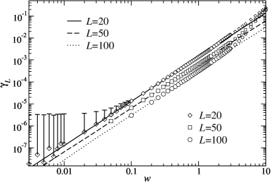
Figure 1: Lyapunov exponent $\gamma_{L}$ as function of disorder strength for energy $E=1.1$ and strip widths $L=20,50,100$. Lines have been computed from (7) with $0.05\%$ error, symbols denote results of TMM calculations (with $0.5\%$ error if there is no error bar). Error bars are drawn on one side only.

The rigorous perturbative formula for the smallest Lyapunov exponent within the band is then, under a hypothesis on the incommensurability of the rotation phases which excludes energies with Kappus-Wegner-type anomalies KapW81 and interior band edges, given by

$$\gamma_{L}\;=\;\frac{w^{2}}{96\,L}\sum_{l,k}\frac{2-\delta_{l,k}}{\sin\eta_{l}\sin\eta_{k}}\;\langle\rho_{L,l}\;\rho_{L,k}\rangle\;+\;{\cal O}(w^{4})\;,$$ (7)

where the sum runs over elliptic channels only (actually, for hyperbolic channels $k$, $\rho_{L,k}(n)$ almost vanishes for $n$ large enough as will be discussed below). For a single channel, this expression reduces to the perturbative 1D result given above if one sets ${\bf\Delta}_{1}=0$ in (2) and then $\mu_{0}=E$ so that $\eta_{0}=k$. We emphasize that only the averaged channel weights of the last frame vector $u_{L}$ enter expression (7). We also remark that the dependence of the error term on $L$ and $E$ remains unspecified.

For a numerical study of (7), one first evaluates the Birkhoff averages $\langle\rho_{L,l}\rho_{L,k}\rangle$ as in (6) by generating random transfer matrices just as in the TMM MilRSU00 . Reporting this into (7) and neglecting the ${\cal O}(w^{4})$ term gives the perturbative values plotted in Fig. 1 (as well as Fig. 2 and 3 below). This was done for a typical energy $E=1.1$ away from internal band edges such that $|\mu_{l}|\neq 2$ for all $l$. For comparison, we also plot the value of $\gamma_{L}$ as evaluated by the standard TMM. Very good agreement is obtained even for rather large values of $w$. For very small $w$, the numerical convergence of the TMM estimates for $\gamma_{L}$ is computationally intensive whereas the convergence of the average channel weights needs about a factor $10^{3}$ less iterations. More stable results can hence be obtained at a fraction of the computational cost. For $L=20$ and $E=1.1$, the validity of the perturbative formula breaks down at about $w\approx 3.0$, for large $L$ a bit earlier. The breakdown happens in the region of crossover from quasi-1D to 2D behavior, i.e. $L\gamma_{L}\approx 1$.

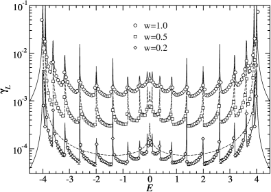
Figure 2: Lyapunov exponent $\gamma_{L}$ as function of energy for disorder $w=0.2,0.5,1.0$ and strip width $L=20$. Solid lines have been computed from (7) with $0.05\%$ error, symbols denote results of TMM calculations with $0.5\%$ error. For $w=0.5$ the dashed solid line was calculated from Eq. (8) and for $w=0.2$ from Eq. (9).

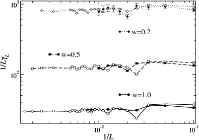
Figure 3: Log-log plot of the reduced localization length $1/L\gamma_{L}$ as function of inverse strip width $1/L$ for energy $E=1.1$ and disorders $w=0.2$ ($\diamond$), $w=0.5$ ($\Box$), and $w=1.0$ ($\circ$). Full symbols denote results of TMM calculations with $0.5\%$ error, open symbols have been computed using (7) with $0.05\%$ error. The lines serve as guide to the eye.

Fig. 2 shows the energy dependence of $\gamma_{L}$ and its perturbative approximation (7). The oscillatory behavior is very well reproduced by the internal band edges corresponding to some eigenmode of ${\bf\Delta}_{L}$, that is the peaks lie precisely on energies $E$ where $|\mu_{l}|=2$ for some $l$ so that ${\sin\eta_{l}}=0$. As the validity of (7) in their vicinity is restricted, the singularities of the perturbative approximation are artificial. In fact, one has to adapt the analysis of DG84 using the normal form of Sch04b to this higher dimensional case. This will be done elsewhere.

Fig. 3 shows the strip width dependence of the reduced localization length in a plot usually used to infer the universal 2D scaling function. The scaling hypothesis AbrALR79 ; KraM93 states that there is a unique scaling function $F$ such that one can find a function $\xi(w)$, also called the 2D localization length, so that all the data $\gamma_{L}(w)$ satisfies $\log\left(\frac{1}{L\gamma_{L}(w)}\right)=F\left[\log\left(\frac{\xi(w)}{L}\right)\right]$. Hence Fig. 3 allows to read off a part of $F$ which is usually difficult to determine numerically because the TMM converges badly for very small $w$. Note that all the data of Fig. 3 lie well inside the quasi-1D regime where $L\gamma_{L}\ll 1$.

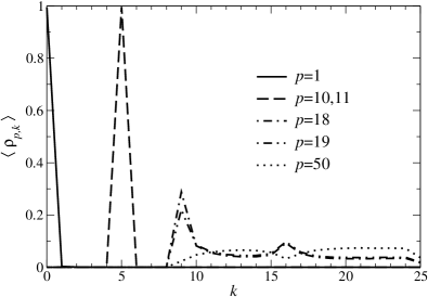
Figure 4: A sample of numerical results for the average channel weights $\langle\rho_{p,k}\rangle$ as function of the channel number $k$ for various frame vectors (index $p$). The strip width is $L=50$, energy $E=1.1$ and disorder $w=0.5$. Hyperbolic frame vectors with $p\leq 17$ have a large $\langle\rho_{p,k}\rangle\sim 1$ for a specific $k$, whereas elliptic frame vectors $p\geq 18$ all have nearly a uniform distribution on elliptic channel indices $9\leq k\leq 25$. The lines serve as guide to the eye.

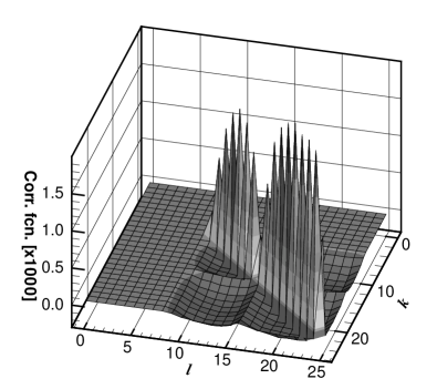
Figure 5: Contour plot of the numerically evaluated correlation function $\langle\rho_{L,l}\rho_{L,k}\rangle-\langle\rho_{L,l}\rangle\langle\rho_{L,k}\rangle$ of the $L$th frame vector plotted as function of channel indices $l,k$ for energy $E=1.1$, disorder $w=0.25$, and strip width $L=50$. The correlation for hyperbolic channel numbers $l,k\leq 8$ is zero.

We now analyze further quantities of the TMM random dynamical system. Fig. 4 shows typical numerical results on the average channel weights. The first frame vectors align with the hyperbolic channels. More precisely, they fill them one after another in order of decreasing dilation exponents. Thus $u_{1}$ completely aligns with the expanding direction of the most hyperbolic channel corresponding to the fundamental of $\Delta_{L}$. Vectors $p=10,11$ fill the doubly degenerate sixth channel. Due to symplectic and orthogonal blocking, the remaining frame vectors have to be in the elliptic channels. In fact, they have a more or less uniform distribution over the elliptic channels (in particular, also the last one $p=50$), only the first elliptic frame vectors $p=18$, $19$ give more weight to channels close to the internal band edges. Moreover, further numerics show that all these distributions are nearly independent of the disorder strength for $w$ sufficiently small enough. Indeed, one can set up a BGGKY-type hierarchy for these distributions Sch03 . The fact that the distribution over the elliptic channels is nearly uniform is a result of the mixing properties of the random potential, because the free dynamics ${\bf R}$ gives no preference to any of the elliptic channels. Fig. 5 shows that the correlations in the calculation of Birkhoff averaged channel weights are very small. Hence, as further approximation, one may factor the stochastic matrix in (7).

Resuming, the numerical results imply that the distribution of the last frame vector is uniform on the elliptic channels, the correlations are weak and all this is uniformly for small $w$. Hence a good approximation for the coefficient in (7) should be obtained upon replacing $\langle\rho_{L,l}\;\rho_{L,k}\rangle$ by $(L_{e})^{-2}$ if $L_{e}$ is the number of elliptic channels. This gives

$$\gamma_{L}\;\approx\;\frac{w^{2}}{96\,L}\;\frac{1}{L_{e}^{2}}\,\sum_{l,k}\frac{2-\delta_{l,k}}{\sin\eta_{l}\sin\eta_{k}}\;,$$ (8)

where the sum still runs over elliptic channels only. This fits well with the results of Fig. 1 and gives a good approximation as shown in Fig. 2 for $w=0.5$, albeit not as good as Eq. (7). For large $L$, one may furthermore neglect the $\delta_{l,k}$ in (8) and approximate the discrete sum by a Riemann integral. Hence, we infer for $E>0$ and large $L$ (but not too large so that $E$ stays away from internal band edges)

$${\gamma_{L}}\approx\frac{w^{2}}{12L}\left(\int_{\eta_{E}\leq\eta\leq\pi}\frac{d\eta}{\pi-\eta_{E}}\,\frac{1}{\sqrt{4-(2\cos\eta+E)^{2}}}\right)^{2},$$ (9)

where we set $\eta_{E}=\arccos(1-{E}/{2})$. Indeed this elliptic integral (of first kind) can be evaluated numerically. Of course, this does not give the rich oscillatory structure for finite $L$ anymore as demonstrated in Fig. 2 for the case $w=0.2$.

We acknowledge financial support by the DFG via SFB 288 and the priority research program “Quanten-Hall Systeme”.

References

- (1) I. Goldsheid, S. Molcanov, L. Pastur, Funct. Anal. Appl. 11, 1 (1977).
- (2) D. J. Thouless, in Ill-condensed Matter, edited by G. Toulouse and R. Balian (North-Holland, Amsterdam, 1979), p. 1.
- (3) L. Pastur, A. Figotin, Spectra of Random and Almost-Periodic Operators, (Springer, Berlin, 1992).
- (4) E. Abrahams, P. W. Anderson, D. C. Licciardello, and T. V. Ramakrishnan, Phys. Rev. Lett. 42, 673 (1979).
- (5) A. MacKinnon and B. Kramer, Phys. Rev. Lett. 47, 1546 (1981); —, Z. Phys. B 53, 1 (1983).
- (6) J.-L. Pichard and G. Sarma, J. Phys. C 14, L127 and L617 (1981).
- (7) J. Fröhlich, T. Spencer, Commun. Math. Phys. 88, 151 (1983).
- (8) M. Aizenman, S. Molchanov, Commun. Math. Phys. 157, 245-278 (1993).
- (9) D. J. Thouless, Phys. Rev. Lett. 39, 1167 (1977).
- (10) C. W. J. Beenakker, Rev. Mod. Phys. 69, 731 (1997).
- (11) H. Schulz-Baldes, Perturbation theory for Lyapunov exponents of an Anderson model on a strip, mp_arc/03-369, to appear in GAFA, (2004).
- (12) In Sch03 , the distribution of the ’s is merely supposed to be centered and of unit variance. The present normalization of the disorder strength is the standard choice in the physics literature.
- (13) P. Bougerol, J. Lacroix, Products of Random Matrices with Applications to Schrödinger Operators, (Birkhäuser, Boston, 1985).
- (14) M. Kappus and F. Wegner, Z. Phys. B 45, 15 (1981).
- (15) F. Milde, R. A. Römer, M. Schreiber, and V. Uski, Eur. Phys. J. B 15, 685 (2000), ArXiv: cond-mat/9911029.
- (16) B. Derrida, E. J. Gardner, J. Physique 45, 1283 (1984).
- (17) H. Schulz-Baldes, Lifshitz tails for the 1D Bernoulli-Anderson model, mp_arc/03-368, to appear in Markow Processes and Related Fields, (2004).
- (18) B. Kramer and A. MacKinnon, Rep. Prog. Phys. 56, 1469 (1993).