Polarization kinetics in ferroelectrics
with regard to fluctuations

Abstract

Polarization in ferroelectrics, described by the Landau-Ginzburg Hamiltonian, is considered, based on a multi-dimensional Fokker-Planck equation. This formulation describes the time evolution of the probability distribution function over the polarization field configurations in the presence of a time dependent external field. The Fokker-Planck equation in a Fourier representation is obtained, which can then be solved numerically for a finite number of modes. Calculation results are presented for one and three modes. These results show the hysteresis of the mean polarization as well as that of the mean squared gradient of the polarization.

Keywords: Ferroelectric, Landau–Ginzburg Hamiltonian, Fokker–Planck equation,
polarization hysteresis.

PACS: 77.80.Dj, 77.80.Fm

1 Introduction

The stochastic description of collective phenomena such as phase transitions is a key theme in solid-state physics. Problems of this kind are nontrivial and are usually solved by means of perturbation theory [1, 2, 3]. Here the kinetics of polarization switching in ferroelectrics is studied, taking into account the spatio-temporal fluctuations of the polarization field given by the Langevin and multi-dimensional Fokker-Planck equations [4, 5]. Simplified approaches are well known [6, 7, 8], for which the static distribution of the polarization is found by minimizing the Landau-Ginzburg type free energy functional. The dynamics and fluctuations of the polarization are usually introduced via equations of mean-field type representing either an approximation or a solution of the appropriate mean-field model [9]. The multi-dimensional Fokker-Planck equation discussed here allows us to consider unlimitedly many nontrivial degrees of freedom for the correlated collective fluctuations of the polarization field, which are lost or roughly treated as uncorrelated in the mean-field approximation. This problem has been studied previously [10, 11] by means of the perturbative Feynman diagram technique. Such an approach, however, only allows the description of the ferroelectric response with respect to an infinitely small external field, rather than polarization reversal (switching) and hysteresis. The latter requires a non-perturbative treatment [12, 13, 14] which, however, is usually done by including some kind of mean-field approximation. In [15, 16, 17] the polarization reversal has been studied based on the classical nucleation theory. At the initial stage, the formation of domains of new phase is considered as one–step Markov process, in which case the domain size can increase or decrease by one unit at a time moment. The obtained in this way distribution over the sizes of small fluctuating domains (or nuclei) is then used to describe the later stage of the domain growth and the polarization reversal. Despite of some simplifications (neglecting nontrivial spatial correlations as well as complicated merging and splitting processes) it gives realistic results [15, 17]. An explicit consideration of the nucleation and growth of domains lies also in the basis of more recent simulations of ferroelectricity in polycrystals and single crystals [18, 19], as well as of combined ferro– and piezo–electric effects [20, 21]. These ideas are applied also to describe experimentally observed features in specific materials [22, 23]. In the present work the Fokker-Planck equation in a Fourier representation, which is suitable for a non-perturbative numerical approach avoiding approximations of the mean-field type, is derived. In principle, it allows to include many nontrivial degrees of freedom, lost in the known simplified approaches, as regards the spatial correlations and fluctuations of the polarization. In practical calculations of this kind, however, only some fluctuation degrees of freedom, that is only a few Fourier modes, can be implemented due to computation time and memory constraints. Nevertheless, such limited calculations can reproduce some important qualitative features and provide test examples to verify possible approximations which would allow the treatment of realistic numbers of modes.

2 Basic equations

We consider a ferroelectric with the Landau-Ginzburg Hamiltonian

$$H=\int\left(\frac{\alpha}{2}P^{2}({\bf x})+\frac{\beta}{4}P^{4}({\bf x})+\frac{c}{2}(\nabla P({\bf x}))^{2}-\lambda({\bf x},t)P({\bf x},t)\right)d{\bf x}\;,$$ (1)

where $P({\bf x},t)$ is the local polarization and $\lambda({\bf x},t)$ is the time-dependent external field. The only configurations of the polarization which are allowed are those corresponding to the cut-off $k<\Lambda$ in Fourier space with $\Lambda=\pi/a$, where $a$ is the lattice constant. The Hamiltonian (1) can be approximated by a sum over discrete cells, where the size of one cell can be larger than the lattice constant. Such cells are small domains with almost constant polarization. Thus the Hamiltonian of a system with volume $V$ is

$$H=\Delta V\sum\limits_{\bf x}\left(\frac{\alpha}{2}P^{2}({\bf x})+\frac{\beta}{4}P^{4}({\bf x})+\frac{c}{2}(\nabla P({\bf x}))^{2}-\lambda({\bf x},t)P({\bf x},t)\right)\;,$$ (2)

where $\Delta V=V/N$ is the volume of one cell and the coordinates of the centers of the cells are given by the set of discrete $d$-dimensional vectors $\bf x\in\mbox{R}^{d}$. The stochastic dynamics of the system is described by the Langevin equation

$$\dot{P}({\bf x},t)=-\gamma\frac{\partial H}{\partial P({\bf x},t)}+\xi({\bf x},t)\;,$$ (3)

where $\xi({\bf x},t)$ is white noise, i.e.

$$\langle\xi({\bf x},t)\xi({\bf x}^{\prime},t^{\prime})\rangle=2\gamma\theta\,\delta_{{\bf x},{\bf x}^{\prime}}\delta(t-t^{\prime})\;.$$ (4)

In the case of Gaussian white noise, the probability distribution function

$$f\left(P\left({\bf x}_{1}\right),P\left({\bf x}_{2}\right),\cdots,P\left({\bf x}_{N}\right),t\right)$$

is given by the Fokker-Planck equation [5]

$$\frac{1}{\gamma}\frac{\partial f}{\partial t}=\sum\limits_{\bf x}\frac{\partial}{\partial P({\bf x})}\left(\frac{\partial H}{\partial P({\bf x})}\,f+\theta\frac{\partial f}{\partial P({\bf x})}\right)\;.$$ (5)

At equilibrium the flux vanishes, which corresponds to the Boltzmann distribution $f\propto\exp(-H/\theta)$ with $\theta=k_{B}T$.

Assuming periodic boundary conditions, we consider the discrete Fourier transform

$$P({\bf x}) = N^{-1/2}\sum\limits_{\bf k}P_{\bf k}e^{i{\bf kx}}$$ (6)

$$P_{\bf k} = N^{-1/2}\sum\limits_{\bf x}P({\bf x})e^{-i{\bf kx}}\;.$$ (7)

The Fourier amplitudes are the complex numbers $P_{\bf k}=P^{\prime}_{\bf k}+iP^{\prime\prime}_{\bf k}$. Since $P({\bf x})$ is real, $P^{\prime}_{-\bf k}=P^{\prime}_{\bf k}$ and $P^{\prime\prime}_{-\bf k}=-P^{\prime\prime}_{\bf k}$ hold. It is supposed that the total number of modes $N$ is an odd number. This means that there is a mode with ${\bf k}={\bf 0}$ and modes with $\pm{\bf k}_{1},\pm{\bf k}_{2},\ldots,\pm{\bf k}_{m}$, where $m=(N-1)/2$ is the number of independent non-zero modes.

The Fokker-Planck equation for the probability distribution function

$$f=f\left(P_{\bf 0},P^{\prime}_{{\bf k}_{1}},P^{\prime}_{{\bf k}_{2}},\ldots,P^{\prime}_{{\bf k}_{m}},P^{\prime\prime}_{{\bf k}_{1}},P^{\prime\prime}_{{\bf k}_{2}},\ldots,P^{\prime\prime}_{{\bf k}_{m}},t\right)$$ (8)

is then

$$\frac{1}{\gamma}\frac{\partial f}{\partial t} = \sum\limits_{{\bf k}\in\Omega}\frac{\partial}{\partial P^{\prime}_{\bf k}}\left\{\frac{1}{2}\left(1+\delta_{{\bf k},{\bf 0}}\right)\left[\frac{\partial H}{\partial P^{\prime}_{\bf k}}f+\theta\frac{\partial f}{\partial P^{\prime}_{\bf k}}\right]\right\}$$ (9)

$$+ \sum\limits_{{\bf k}\in\bar{\Omega}}\frac{\partial}{\partial P^{\prime\prime}_{\bf k}}\left\{\frac{1}{2}\left[\frac{\partial H}{\partial P^{\prime\prime}_{\bf k}}f+\theta\frac{\partial f}{\partial P^{\prime\prime}_{\bf k}}\right]\right\}\;,$$

where $P^{\prime}_{\bf 0}\equiv P_{\bf 0}$, $\bar{\Omega}$ is the set of $m$ independent non-zero wave vectors and $\Omega$ includes ${\bf k}={\bf 0}$. Here the Fourier transformed Hamiltonian is given by

$$H = \Delta V\left(\frac{1}{2}\sum\limits_{\bf k}\left(\alpha+c{\bf k}^{2}\right)\mid P_{\bf k}\mid^{2}+\frac{\beta}{4}N^{-1}\sum\limits_{{\bf k}_{1}+{\bf k}_{2}+{\bf k}_{3}+{\bf k}_{4}={\bf 0}}P_{{\bf k}_{1}}P_{{\bf k}_{2}}P_{{\bf k}_{3}}P_{{\bf k}_{4}}\right.$$ (10)

$$\hskip 34.44434pt-\left.\sum\limits_{\bf k}\lambda_{-\bf k}(t)P_{\bf k}\right)\;.$$

Some of the variables in Eq. (10) are dependent according to $P^{\prime}_{-\bf k}\equiv P^{\prime}_{\bf k}$ and $P^{\prime\prime}_{-\bf k}\equiv-P^{\prime\prime}_{\bf k}$. Here $\lambda_{\bf k}(t)=\lambda^{\prime}_{\bf k}(t)+i\lambda^{\prime\prime}_{\bf k}(t)$ is the Fourier transform of $\lambda({\bf x},t)$. The Fokker-Planck equation (9) can be written explicitly as

$$\frac{1}{\gamma}\frac{\partial f}{\partial t} = \sum\limits_{{\bf k}\in\Omega}\frac{\partial}{\partial P^{\prime}_{\bf k}}\left\{\Delta V\,f\left[\left(\alpha+c{\bf k}^{2}\right)P^{\prime}_{\bf k}+\beta S^{\prime}_{\bf k}-\lambda^{\prime}_{\bf k}(t)\right]+\frac{\theta}{2}\left(1+\delta_{{\bf k},{\bf 0}}\right)\frac{\partial f}{\partial P^{\prime}_{\bf k}}\right\}$$ (11)

$$+ \sum\limits_{{\bf k}\in\bar{\Omega}}\frac{\partial}{\partial P^{\prime\prime}_{\bf k}}\left\{\Delta V\,f\left[\left(\alpha+c{\bf k}^{2}\right)P^{\prime\prime}_{\bf k}+\beta S^{\prime\prime}_{\bf k}-\lambda^{\prime\prime}_{\bf k}(t)\right]+\frac{\theta}{2}\frac{\partial f}{\partial P^{\prime\prime}_{\bf k}}\right\}\;,$$

where

$$S^{\prime}_{\bf k} = N^{-1}\sum\limits_{{\bf k}_{1}+{\bf k}_{2}+{\bf k}_{3}={\bf k}}\left\{P^{\prime}_{{\bf k}_{1}}P^{\prime}_{{\bf k}_{2}}P^{\prime}_{{\bf k}_{3}}-3P^{\prime}_{{\bf k}_{1}}P^{\prime\prime}_{{\bf k}_{2}}P^{\prime\prime}_{{\bf k}_{3}}\right\}\;,$$ (12)

$$S^{\prime\prime}_{\bf k} = N^{-1}\sum\limits_{{\bf k}_{1}+{\bf k}_{2}+{\bf k}_{3}={\bf k}}\left\{-P^{\prime\prime}_{{\bf k}_{1}}P^{\prime\prime}_{{\bf k}_{2}}P^{\prime\prime}_{{\bf k}_{3}}+3P^{\prime\prime}_{{\bf k}_{1}}P^{\prime}_{{\bf k}_{2}}P^{\prime}_{{\bf k}_{3}}\right\}\;.$$ (13)

3 Spatially homogeneous case

The simplest case is a spatially homogeneous polarization for which only the ${\bf k}={\bf 0}$ mode is retained in (11) with a spatially homogeneous external field $\lambda({\bf x},t)=\lambda_{\bf 0}(t)=A\sin(\omega t)$. In this case we have

$$\frac{1}{\gamma}\frac{\partial f}{\partial t}=\frac{\partial}{\partial P_{\bf 0}}\left\{V\,f\left[\alpha P_{\bf 0}+\beta P_{\bf 0}^{3}-A\sin(\omega t)\right]+\theta\frac{\partial f}{\partial P_{\bf 0}}\right\}\;.$$ (14)

The mean value of the zero-th Fourier amplitude

$$\bar{P}_{\bf 0}=\int\limits_{-\infty}^{\infty}P_{\bf 0}f\left(P_{\bf 0},t\right)dP_{\bf 0}$$ (15)

is the mean polarization $\bar{P}$ in this case, as follows from (6).

4 Quasi one-dimensional case with homogeneous
external field

We shall further consider a quasi one-dimensional case, for which a three-dimensional ferroelectric sample is stretched out in the $x$-direction, i.e. $L_{x}\gg L_{y}$ and $L_{x}\gg L_{z}$ hold for the linear sizes. In this case we assume that the polarization, as well as the external field, depend only on the $x$ coordinate. This means that the wave vectors also have only one non-vanishing component, which is a scalar quantity $k_{n}=\left(2\pi/L_{x}\right)\cdot n$, where $n=0,\pm 1,\pm 2,\ldots,\pm m$. From now on, we shall omit the vector notation in this quasi one-dimensional case.

As a first step, we shall include only one ($m=1$) independent non-zero wave vector $k_{L}=2\pi/L_{x}$ (in total $N=3$ wave vectors $k=-k_{L},0,k_{L}$) and a homogeneous external field

$$\lambda(x,t)=\frac{1}{\sqrt{3}}\lambda_{0}(t)=\frac{1}{\sqrt{3}}A\sin(\omega t).$$ (16)

Furthermore, we shall assume that the probability distribution function in real space is translation invariant at the initial time. Due to the translational symmetry of the model, translation invariance then also holds at all later times. In the Fourier representation, this means that the probability distribution function depends on the modulus of $P_{{k_{1}}}$, but not on its phase. Thus we have

$$f=f\left(P_{0},P^{\prime}_{{k_{1}}},P^{\prime\prime}_{{k_{1}}},t\right)=\frac{\hat{f}\left(P_{0},\mid P_{{k_{1}}}\mid,t\right)}{2\pi\mid P_{{k_{1}}}\mid}\;,$$ (17)

where $\hat{f}\left(P_{0},\mid P_{{k_{1}}}\mid,t\right)$ is the probability density in the $\left(P_{0},\mid P_{{k_{1}}}\mid\right)$ space and which obeys the Fokker-Planck equation

$$\frac{1}{\gamma}\frac{\partial\hat{f}}{\partial t} = \frac{\partial}{\partial P_{0}}\left\{\Delta V\,\hat{f}\left[\alpha P_{0}+\beta\left(\frac{1}{3}P_{0}^{3}+2P_{0}\mid P_{{k_{1}}}\mid^{2}\right)-A\sin(\omega t)\right]+\theta\frac{\partial\hat{f}}{\partial P_{0}}\right\}$$ (18)

$$+ \frac{\partial}{\partial\mid P_{{k_{1}}}\mid}\left\{\Delta V\,\hat{f}\left[\left(\alpha+ck_{1}^{2}\right)\mid P_{{k_{1}}}\mid+\beta\left(\mid P_{{k_{1}}}\mid^{3}+P_{0}^{2}\mid P_{{k_{1}}}\mid\right)\right]\right.$$

$$+ \left.\frac{\theta}{2}\left[\frac{\partial\hat{f}}{\partial\mid P_{{k_{1}}}\mid}-\frac{\hat{f}}{\mid P_{{k_{1}}}\mid}\right]\right\}\;.$$

Since $f$ is finite, $\hat{f}$ vanishes at $\mid P_{{k_{1}}}\mid=0$. The physical boundary conditions correspond to zero flux at the boundaries $P_{0}=\pm\infty$, $\mid P_{{k_{1}}}\mid=0$ and $\mid P_{{k_{1}}}\mid=\infty$. An appropriate initial condition has to be chosen which fulfils these relations, e.g. $\hat{f}\left(P_{0},\mid P_{{k_{1}}}\mid,0\right)\propto\mid P_{{k_{1}}}\mid\exp\left(-a_{0}P_{0}^{2}-a_{1}\mid P_{{k_{1}}}\mid^{2}\right)$.

5 Numerical results

The Fokker-Planck Eq. (11) has been solved numerically in the quasi-one dimensional case for which the wave vector has only one component $k\equiv k_{x}$, in the spatially homogeneous approximation with only the $n=0$ $\left(k_{x}=0\right)$ mode (in total $N=1$ modes), as well as in the next higher order approximation for which the spatial distribution of the polarization field is taken into account by including $n=0,\mp 1$ (in total $N=3$ modes) with $k_{n}=k_{L}\,n$.

At first, rewriting the Eq. (11) in the following form:

$$\frac{1}{\gamma}\frac{\partial f}{\partial t}=\frac{\partial}{\partial P^{\prime}_{k_{0}}}J_{0}^{{}^{\prime}}+\frac{\partial}{\partial P^{\prime}_{k_{1}}}J_{1}^{{}^{\prime}}+\frac{\partial}{\partial P^{\prime\prime}_{k_{1}}}J_{1}^{{}^{\prime\prime}},$$ (19)

where (for $\alpha<0$):

$$J_{n}^{\diamond}=\Delta V\,\left[\left(|\alpha|-c{k_{n}}^{2}\right)P^{\diamond}_{k_{n}}-\beta S^{\diamond}_{k_{n}}+\lambda^{\diamond}_{k_{n}}(t)\right]f-r_{n}^{\diamond}\frac{\theta}{2}\frac{\partial f}{\partial P^{\diamond}_{k_{n}}},$$ (20)

$$r_{n}^{\diamond}=\left\{\begin{array}[]{r}1+\delta_{k_{n},0};\diamond=^{\prime}\\ 1;\diamond=^{\prime\prime}\end{array}\right.,\quad n=0,1.$$ (21)

Then, by using a special exponential-type substitution for the distribution function:

$$f=W_{k_{n}}^{\diamond}\exp\left\{\int_{p_{0}}^{P^{\diamond}_{k_{n}}}\frac{2\Delta V}{r_{n}^{\diamond}\,\theta}\left[\left(|\alpha|-c{k_{n}}^{2}\right)p-\beta S^{\diamond}_{k_{n}}+\lambda^{\diamond}_{k_{n}}(t)\right]dp\right\},$$ (22)

where $W_{k_{n}}^{\diamond}$ is a normalization function and $p_{0}$ is a real number (similarly as in [24], it can be shown that $W_{k_{n}}^{\diamond}$ and $p_{0}$ should not affect final coefficients of a difference scheme), a monotone, exponential difference scheme has been developed:

$$\left(\Lambda\left(\eta\right)f^{l+1}\right)_{\bf i}=\sum_{n=0}^{1}\frac{1}{h_{i_{n}^{{}^{\prime}}}^{*}}\left(A_{\bf i}^{n}\right)^{{}^{\prime}}f^{l+1}_{{\bf i}-{\bf e}_{n}^{{}^{\prime}}}+\frac{1}{h_{i_{n}^{{}^{\prime}}}^{*}}\left(B_{\bf i}^{n}\right)^{{}^{\prime}}f^{l+1}_{{\bf i}+{\bf e}_{n}^{{}^{\prime}}}-\left(Q_{{\bf i}}^{n}\right)^{{}^{\prime}}f_{{\bf i}}^{l+1}+$$

$$\sum_{n=-1}^{-1}\frac{1}{h_{i_{n}^{{}^{\prime\prime}}}^{*}}\left(A_{{\bf i}}^{n}\right)^{{}^{\prime\prime}}f^{l+1}_{{\bf i}-{\bf e}_{n}^{{}^{\prime\prime}}}+\frac{1}{h_{i_{n}^{{}^{\prime\prime}}}^{*}}\left(B_{{\bf i}}^{n}\right)^{{}^{\prime\prime}}f^{l+1}_{{\bf i}+{\bf e}_{n}^{{}^{\prime\prime}}}-\left(Q_{{\bf i}}^{n}\right)^{{}^{\prime\prime}}f_{{\bf i}}^{l+1}=\frac{1}{\gamma}\frac{f_{{\bf i}}^{l+1}-f_{{\bf i}}^{l}}{\tau_{l+1}},$$ (23)

$$\quad\quad\quad\quad\quad\quad\quad\quad\quad\quad\quad 0<i_{n}^{\diamond}<I_{n}^{\diamond},$$

with coefficients:

$$\left(Q_{{\bf i}}^{n}\right)^{\diamond}=\frac{1}{h^{*}_{i_{n}^{\diamond}}}\left(A_{{\bf i}+{\bf e}_{n}^{\diamond}}^{n}\right)^{\diamond}+\frac{1}{h^{*}_{i_{n}^{\diamond}}}\left(B_{{\bf i}-{\bf e_{n}^{\diamond}}}^{n}\right)^{\diamond},$$ (24)

$$\left(A_{{\bf i}}^{n}\right)^{\diamond}=\frac{\theta\,r_{n}^{\diamond}}{2}\left(\eta\right)_{{\bf i}-1/2{\bf e_{n}^{\diamond}}}\frac{1}{h_{i_{n}^{\diamond}}\left(\exp\left(\left(\eta\right)_{{\bf i}-1/2{\bf e_{n}^{\diamond}}}\right)-1\right)},$$ (25)

$$\left(B_{{\bf i}}^{n}\right)^{\diamond}=\frac{\theta\,r_{n}^{\diamond}}{2}\left(\eta\right)_{{\bf i}+1/2{\bf e_{n}^{\diamond}}}\frac{\exp\left(\left(\eta\right)_{{\bf i}+1/2{\bf e_{n}^{\diamond}}}\right)}{h_{i_{n}^{\diamond}+1}\left(\exp\left(\left(\eta\right)_{{\bf i}+1/2{\bf e_{n}^{\diamond}}}\right)-1\right)},$$ (26)

$$\left(\eta\right)_{{\bf i}-1/2{\bf e_{n}^{\diamond}}}=\frac{2\Delta V}{\theta\,r_{n}^{\diamond}}\left(\left(-|\alpha|+c{k_{n}}^{2}\right)P_{k_{n}}^{\diamond}+\beta S_{k_{n}}^{\diamond}-\lambda_{k_{n}}(t_{l+1})\right)_{{\bf i}-1/2{\bf e_{n}^{\diamond}}}h_{i_{n}^{\diamond}},$$ (27)

where ${\bf i}=(i_{0},i_{1}^{{}^{\prime}},i_{1}^{{}^{\prime\prime}})$ and ${\bf e}_{n}^{\diamond}$ is unit vector in the $i_{n}^{\diamond}$ direction, $l$ is the time index, $h$ is the polarization space step and $\tau$ is the time step.

Elaborated difference scheme (23) - (27) has a first order truncation error in time and a second order truncation error in space, when $|\eta|\rightarrow 0$. In the limit $|\eta|\rightarrow\infty$, so that transport is advection dominated, when $\theta\rightarrow 0$, the difference scheme (23) - (27) has first order truncation errors in time and space.

For one dimensional case, when $N=1$, difference scheme (23) - (27) coincides with elaborated in [25]. As it was shown [25], for $|\eta|\rightarrow 0$ and $|\eta|\rightarrow\infty$ one dimensional exponential scheme becomes absolutely stable. Here in order to control the precision (stability) of the calculations we adopted a linear prognosis criterion. Accordingly, we required that the linear prognosis at each time step should not deviate from the numerical solution to a given precision, which varied from $\varepsilon_{l}=2\cdot 10^{-4}$ to $\varepsilon_{f}=5\cdot 10^{-4}$. If this precision criterion was met, then the time step was kept constant. The time step was increased if the linear prognosis deviation was less than $\varepsilon_{l}$, and it was decreased if the linear prognosis deviation was greater than $\varepsilon_{f}$.

Elaborated absolute monotone scheme (23) - (27) for the Fokker–Planck Eq. (11) has been implemented on parallel processing for one and three polarization space dimensions, when $N=1$ and $N=3$. A parallel code version of program is written by implementing MPI programming technology in FORTRAN and using ScaLAPACK (SUN S3L) linear algebra solver.

In contrast to the quasi-one dimensional case discussed in Sec. 4, here we consider homogeneous as well as non-homogeneous external fields based on (11) as a generic equation. This equation reduces to (14) for $N=1$. In the case for which the field is spatially homogeneous it is given by $\lambda_{0}(t)=A\sin(\omega t)=A^{\prime}\sqrt{N}$ $\sin(\omega t)$, the other Fourier components being zero, whereas the non-homogeneous field is chosen such that $\lambda_{0}(t)=\lambda^{\prime}_{k_{1}}(t)=\lambda^{\prime\prime}_{k_{1}}(t)=A^{\prime}\sqrt{N}\sin(\omega t)$. In the coordinate representation, this corresponds to $\lambda(x,t)=A^{\prime}\sin(\omega t)$ in the homogeneous case and to

$$\lambda(x,t)=A^{\prime}\sin(\omega t)\\ \left[1+2\sqrt{2}\cos(k_{1}x+\pi/4)\right]$$

in the non-homogeneous case. Note that, according to (6), the mean polarization is given by $\bar{P}=\bar{P}_{0}/\sqrt{N}$. We shall also compute the mean-squared gradient of the polarization $\overline{(\nabla P)^{2}}$, which is given by

$$\overline{{(\nabla P)}^{2}}=N^{-1}\sum\limits_{\bf k}{\bf k}^{2}\overline{{\left|P_{\bf k}\right|}^{2}}=N^{-1}\sum\limits_{\bf k}k^{2}\left(\overline{{P^{\prime}_{\bf k}}^{2}}+\overline{{P^{\prime\prime}_{\bf k}}^{2}}\right)$$ (28)

in general. In our quasi one-dimensional case the sum over ${\bf k}$ reduces to the sum over $k=-k_{L},0,k_{L}$.

In the Eq. (11) expressions for $S$ were given by $S_{0}=P_{0}^{3}$ for $N=1$, and for $N=3$ these are:

$$S_{0} = \frac{1}{3}\left(P_{0}^{{}^{\prime}}\right)^{3}+2P_{0}^{{}^{\prime}}\left(\left(P_{k_{1}}^{{}^{\prime}}\right)^{2}+\left(P_{k_{1}}^{{}^{\prime\prime}}\right)^{2}\right),$$ (29)

$$S_{k_{1}}^{{}^{\prime}} = \left(P_{k_{1}}^{{}^{\prime}}\right)^{3}+P_{k_{1}}^{{}^{\prime}}\left(\left(P_{0}^{{}^{\prime}}\right)^{2}+\left(P_{k_{1}}^{{}^{\prime\prime}}\right)^{2}\right),$$ (30)

$$S_{k_{1}}^{{}^{\prime\prime}} = \left(P_{k_{1}}^{{}^{\prime\prime}}\right)^{3}+P_{k_{1}}^{{}^{\prime\prime}}\left(\left(P_{0}^{{}^{\prime}}\right)^{2}+\left(P_{k_{1}}^{{}^{\prime}}\right)^{2}\right).$$ (31)

The numerical calculations have been performed within the interval $[-3.5,3.5]$ for each Fourier amplitude ($P_{0}$ for $N=1$ and $P_{0}$, $P^{\prime}_{k_{1}}$, $P^{\prime\prime}_{k_{1}}$ for $N=3$) with the boundary condition $f=0$ at the borders of this domain. The parameter values are $\gamma=V=\beta=1$, $L_{x}=7$, $\alpha=-1$, $\theta=0.05$, $A^{\prime}=0.5$ (i.e. $A=0.5\sqrt{N}$) and $\omega=10^{-3}$. The initial condition

$$f\left(P_{0},0\right)=\frac{1}{\sqrt{2\pi}\sigma}\exp\left(-\frac{\left(P_{0}-\tilde{P}\right)^{2}}{2\sigma^{2}}\right)$$ (32)

has been used in the spatially homogeneous ($N=1$) case and has been modified to

$$f\left(P_{0},P^{\prime}_{k_{1}},P^{\prime\prime}_{k_{1}},0\right)=\frac{1}{(2\pi)^{3/2}\sigma^{3}}\exp\left(-\frac{\left(P_{0}-\tilde{P}\right)^{2}+{P^{\prime}_{k_{1}}}^{2}+{P^{\prime\prime}_{k_{1}}}^{2}}{2\sigma^{2}}\right)$$ (33)

in the other case of $N=3$ modes, with $\sigma=0.3$, $\tilde{P}=-1$ for $P_{0}<0$ and $\tilde{P}=1$ for $P_{0}>0$.

The calculated mean polarization in the coordinate space $\bar{P}=\bar{P}_{0}/\sqrt{N}$, which depends on the homogeneous external field represented by $\lambda_{0}(t)$, forms a hysteresis loop, as shown in Fig. 1, where the results for $N=1$ (dot-dashed curve) and $N=3$ (solid curve) are compared. In the second case the spatial distribution of the polarization, generally, is nonhomogeneous. The insertions in Fig. 1 illustrate qualitatively some of possible or typical polarization distributions at different locations on the hysteresis loop.

Figure 1: The polarization hysteresis: the mean polarization $\bar{P}$ vs. normalized external field $\lambda_{0}(t)/A$ calculated numerically for the parameter values $\gamma=V=\beta=1$, $\alpha=-1$, $\theta=0.05$, $A=0.5\sqrt{N}$ and $\omega=10^{-3}$. The solid and dot-dashed lines represent the numerical results for $N=3$ and $N=1$ Fourier modes, respectively. The insertions illustrate possible spatial distributions of the polarization at different locations on the hysteresis loop.

As can be seen, the inclusion of $N=3$ modes only slightly changes the behaviour of the mean polarization as compared with the homogeneous approximation with only the zero mode $k=0$ included ($N=1$ case). The hysteresis loop becomes narrower for $N=3$. This is clear physically, since $N=3$ additional degrees of freedom for the fluctuations in the polarization make reversal of the polarization easier. This phenomenon is related to the known Landauer paradox. Namely, the observed coercive field in real ferroelectrics is much smaller than that calculated assuming a spatially homogeneous switching of the polarization. It is well known that switching in ferroelectrics is a process driven by the nucleation and growth of domains of different polarization [15, 17, 19, 22]. Hence, the above mentioned effect of narrowing the hysteresis loop should be even much stronger for appropriate system parameters and larger number of Fourier modes $N$, allowing to describe the domain structure realistically.

The effect of non-homogeneity of the external field on the polarization hysteresis can be seen in Fig. 2, where numerical results for the homogeneous (solid curve) and the above discussed non-homogeneous (dashed curve) fields are compared in the three mode ($N=3$) approximation.

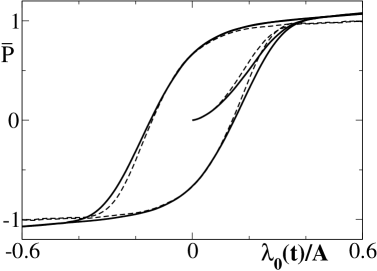
Figure 2: The polarization hysteresis: the mean polarization $\bar{P}$ vs. $\lambda_{0}(t)/A$ calculated numerically for $N=3$ Fourier modes. The solid and the dashed lines represent the results for a homogeneous and non-homogeneous external field, respectively.

The maximum values of $\mid\bar{P}\mid$ are somewhat smaller for the non-homogeneous field. This is related to the fact that the non-homogeneous field

$$\lambda(x,t)=A^{\prime}\sin(\omega t)\left[1+2\sqrt{2}\cos(k_{1}x+\pi/4)\right]$$ (34)

changes sign depending on the coordinate $x$ in such a way that it is positive in $61.5\%$ of the volume and negative in the rest, or vice versa. This means that the polarization, with a large probability, has an opposite sign in the smaller part of the volume, which reduces the modulus of the mean polarization.

In contrast to the spatially homogeneous approximation with $N=1$, inclusion of the non-zero modes allows us to evaluate not only the mean polarization, but also the mean squared gradient of the polarization (28), which is a measure of the spatial inhomogeneity of $P(x,t)$. The hysteresis loop for this quantity, calculated for $N=3$ for the homogeneous external field, is shown in Fig. 3.

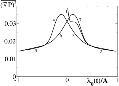
Figure 3: The mean squared gradient of the polarization $\overline{(\nabla P)^{2}}$ vs. $\lambda_{0}(t)/A$ calculated numerically for $N=3$ Fourier modes for the case of a homogeneous external field. The pieces of the hysteresis loop are numbered in order of increasing time.

An interesting feature is that $\overline{{(\nabla P)}^{2}}$ has maxima at times which roughly correspond to those at which the fastest switching of the mean polarization takes place. This provides evidence that the polarization switching quite often, with a remarkable probability, is accompanied by formation of a spatially inhomogeneous structure. The insertions in Fig. 1 illustrate such a scenario. By including more Fourier modes, this eventually could be identified with a domain-like structure. This is the most probable scenario expected from the known studies of the polarization reversal as a nucleation and domain growth process (see, e. g., [15, 17, 19] and references therein).

In Fig. 4, the $\overline{{(\nabla P)}^{2}}$ hysteresis loop is plotted for the non-homogeneous external field. The maxima related to the polarization switching are observed in this case too. Contrary to the case for the homogeneous field, which tends to order the polarization in one direction, the sign alternating non-homogeneous field forces the formation of a non-uniform spatial distribution in the polarization $P(x,t)$.

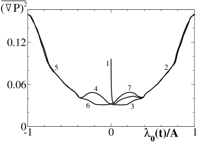
Figure 4: The mean squared gradient of polarization $\overline{(\nabla P)^{2}}$ vs $\lambda_{0}(t)/A$ calculated numerically for $N=3$ Fourier modes for the case of the non-homogeneous external field. Pieces of the hysteresis loop are numbered in order of increasing time.

It can be seen from Figs. 3 and 4 that the mean squared gradient of $P(x,t)$ decreases at the largest absolute values of the field if the field is homogeneous (Fig. 3) and, remarkably, increases for the non-homogeneous field (Fig. 4).

6 Conclusions

In the present work a multi-dimensional Fokker-Planck equation has been derived which describes the kinetics of polarization switching in a ferroelectric in the presence of an external field. The probability distribution function for this equation depends on a set of Fourier amplitudes. Calculations were performed for a spatially homogeneous approximation retaining only the zero mode ${\bf k}={\bf 0}$, as well as for three Fourier modes ($k=-k_{L},0,k_{L}$) for both homogeneous and non-homogeneous external fields. The hysteresis of the mean polarization $\bar{P}$ and of the mean squared gradient of the polarization $\overline{(\nabla P)^{2}}$ were calculated and compared. In particular, it was found that the $\bar{P}$ hysteresis loop becomes slightly narrower when more Fourier modes are included. This loop is qualitatively the same as that observed in real ferroelectrics. The mean squared gradient of polarization is a measure of its inhomogeneity. The hysteresis loop of $\overline{(\nabla P)^{2}}$ provides evidence that polarization switching is accompanied by an increased spatial inhomogeneity of $P(x,t)$, as expected from the known theoretical approaches describing the polarization reversal as a nucleation and growth of domains.

Although only a few Fourier modes were included in the actual calculations, the problem was treated non-perturbatively and without the mean-field approximation. More precisely, our calculations were based on exact equations for the probability distribution function in the case for which the Hamiltonian (10) contains a given number of modes. The present results thus can be used to test various possible approximations.

7 Acknowledgements

This work was carried out under the HPC-EUROPA project (RII3-CT-2003-506079), with the support of the European Community - Research Infrastructure Action under the FP6 ”Structuring the European Research Area” Programme.

References

- [1] Shang-Keng Ma, Modern Theory of Critical Phenomena, W.A. Benjamin, Inc., New York, 1976
- [2] J. Zinn-Justin, Quantum Field Theory and Critical Phenomena, Clarendon Press, Oxford, 1996
- [3] J. Kaupužs, Ann. Phys. (Leipzig) 10, 299 (2001)
- [4] G. Parisi, N. Sourlas, Phys. Rev. Lett. 43, 744 (1979)
- [5] H. Haken, Synergetics, Springer-Verlag, Berlin/ Heidelberg/New York, 1978
- [6] J-M. Liu, Q. C. Li, W. M. Wang, X. Y. Chen, G. H. Cao, X. H. Liu, Z. G. Liu, J. Phys.: Condens. Matter 13, L153, 2001
- [7] P. Talkner, N. J. Phys. 1, 4.1–4.25, 1999
- [8] Y. Shih, Wei-Heng Shih, Ilhan A. Aksay, Phys. Rev. B 50, 15575 (1994)
- [9] M. Shiino, Phys. Rev. A 36, 2393 (1986)
- [10] J. Kaupužs, Phys. Stat. Sol. 195, 325 (1996)
- [11] J. Kaupužs, E. Klotins, Ferroelectrics 296, 239 (2003)
- [12] N. Drozdov, M. Morillo, Phys. Rev. E 54, 3304 (1995)
- [13] E. Klotins, Physica A 340, 196 (2004)
- [14] E. Klotins, J. Kaupužs, Journal of European Ceramical Society 25, 2553 (2005)
- [15] S. A. Kukushkin, A. V. Osipov, Phys. Rev. B 65, 174101 (2002)
- [16] S. A. Kukushkin, A. V. Osipov, Physics of the Solid State 43, 82 (2001)
- [17] S. A. Kukushkin, A. V. Osipov, Physics of the Solid State 43, 90 (2001)
- [18] S. Choudhury, Y. L. Li, C. E. Krill, L. Q. Chen, Acta Materialia 53, 5313 (2005)
- [19] S. Choudhury, Y. L. Li, C. E. Krill, L. Q. Chen, Acta Materialia 55, 1415 (2007)
- [20] W. Zhang, K. Bhattacharya, Acta Materialia 53, 185 (2005)
- [21] W. Zhang, K. Bhattacharya, Acta Materialia 53, 199 (2005)
- [22] M. Iwata, T. Morishita, R. Aoyagi, M. Maeda, I. Suzuki, N. Yasuda, Ferroelectrics 355, 28 (2007)
- [23] E. Milov, V. Milov, B. Strukov, K. Ymazaki, Y. Uesu, Ferroelectrics 341, 39 (2006)
- [24] B. S. Polsky, J. S. Rimshans, Solid State Electron. 29, 321 (1986)
- [25] J. Kaupuzs, J. Rimshans, N. Smyth, In: ”Electromagnetic Fields in Mechatronics, Electrical and Electronic Engineering”, Proc. of ISEF’05, IOS Press, 58 (2006).