Universal Breakdown of Elasticity at the Onset of Material Failure

Abstract

We show that, in the athermal quasi-static deformation of amorphous materials, the onset of failure is accompanied by universal scalings associated with a divergence of elastic constants. A normal mode analysis of the non-affine elastic displacement field allows us to clarify its relation to the zero-frequency mode at the onset of failure and to the crack-like pattern which results from the subsequent relaxation of energy.

Experiments on nanoindentation of metallic glasses SchuhN03 , on granular materials MillerOB96 and on foams PrattD03 , demonstrate that at very low temperature and strain rates, the microstructural mechanisms of deformation involve highly intermittent stress fluctuations. These fluctuations can be accessed in molecular dynamics simulations, but are best characterized numerically via “exact” implementation of a-thermal quasi-static deformation: alternating elementary steps of affine deformation with energy relaxation MaedaT78 permits one to constrain the system to reside in a local energy minimum (inherent structure) at all times. As illustrated in figure 1, macroscopic stress fluctuations arise from a series of reversible (elastic) branches corresponding to deformation-induced changes of local minima. These branches are interrupted by sudden irreversible (plastic) events which occur when the inherent structure annihilates during a collision with a saddle point. MalandroL99 These transitions constitute the most elementary mechanism of deformation and failure for disordered materials at low temperature.

Figure 1: Stress (top) and shear modulus (bottom) for a small strain interval about a strain of $.3$. Left: fixed strain steps of size $10^{-4}$; Right: convergence to the yield point (circled on the left) with decreasing strain step.

Using this quasi-static protocol, recent studies of both elasticity tanguy02 and plasticity MalandroL99 , could identify important properties of elasto-plastic behavior which arise solely from the geometrical structure of the potential energy landscape. Tanguy et al tanguy02 have observed that, following reversible (elastic) changes of the inherent structures, molecules undergo large scale non-affine displacements. They have shown these non-affine displacements to be related to the breakdown of classical elasticity at small scales and to quantitative differences between measured Lamé constants and their Born approximation. Malandro and Lacks MalandroL99 have shown that the destabilization of a minimum occurs through shear-induced collision with a saddle. At the collision, a single normal mode sees its eigenvalue going to zero. Building on this work, we studied the irreversible (plastic) event following the disappearance of an inherent structure: subsequent material deformation in search of a new minimum involves non-local displacement fields –in the likeness of nascent cracks– controlled by long-range elastic interactions. MaloneyL04

Several molecular displacement fields thus appear to be closely related to the geometrical structure of the potential energy landscape: (i) non-affine displacements along elastic branches, (ii) the single normal mode controlling the annihilation of an inherent structure, and (iii) the overall deformation occurring during an irreversible event. In order to piece together a complete picture of elasto-plasticity at the nanoscale, we need to understand the relation between these different fields and ask how elastic behavior breaks down at the onset of failure. It is thus a study of incipient plasticity –that is the onset of irreversible deformation– that we wish to perform. Here, the structural disorder is expected to control the onset of failure: this situation is somehow opposite to homogeneous defect nucleation in crystals, li03 where failure is controlled by Hill’s continuum condition. hill62

We base our approach on exact microscopic expressions for the non-affine corrections to elasticity in disordered solids, wallace72 ; lutsko88 which have entirely been overlooked in recent works. Here, we put such analytical tractations in perspective with the recent numerical developments. We derive an exact formulation for the non-affine displacement fields, and construct a normal mode decomposition therefrom. This analytical framework permits us to evidence that the lowest frequency normal mode dominates the non-affine elastic displacement field close to a plastic transition. We then show that at any plastic transition point, energy, stress, and the vibration frequencies display a singular, universal, behavior associated with a divergence of the elastic constants. The normal mode analysis of the subsequent cascade shows that the low frequency modes active at incipient plasticity are superseded by long-range elastic interactions in the latter stages of an irreversible event.

We consider in this work a molecular system in a periodic cell. The geometry of the cell is determined by the matrix $h$ whose columns are the Bravais vectors. ray84 ; Ray85 The affine deformation of the cell between configurations $h_{0}$ and $h$ is characterized by the Green-St Venant strain tensor, ${\underline{\underline{\epsilon}}}=\frac{1}{2}\left((h_{0}^{-1})^{T}.h^{T}.h.h_{0}^{-1}-1\right)$, which governs the elongation of a vector $\mathring{\vec{x}}\to\vec{x}$, as $\vec{x}^{2}=\mathring{\vec{x}^{2}}+2\,\mathring{\vec{x}^{T}}.{\underline{\underline{\epsilon}}}.\mathring{\vec{x}}$. As the energy functional generally depends only on the set of interparticle distances, it can be parameterized as ${\cal U}(\{\mathring{\vec{r}_{i}}\},{\underline{\underline{\epsilon}}})$ where $\{\mathring{\vec{r}_{i}}\}$ are the positions of the particles in a reference cell. barron65 ; wallace72 Varying, ${\underline{\underline{\epsilon}}}$ for fixed $\{\mathring{\vec{r}_{i}}\}$ corresponds to an affine displacement of the molecules in real space.

To start, let’s contemplate more closely the athermal, quasi-static algorithm. Deformation, ${\underline{\underline{\epsilon}}}(\gamma)$, is enforced by moving the Bravais axes of the periodic cell; $\gamma$ is introduced as rescaled coordinate which measures the amount of deformation from some reference state. In practice ${\underline{\underline{\epsilon}}}(\gamma)$ corresponds to either pure shear or pure compression. Formally, the limit $h_{0}=h$ (or $\gamma\to 0$) is often appropriate to define stresses and elastic constant around a (possibly stressed) reference state. Once a choice of $h_{0}$ is made, the algorithm tracks in the reference cell a trajectory $\{\mathring{\vec{r}_{i}}\}(\gamma)$, which is implicitly defined by demanding that the system remain in mechanical equilibrium: wallace72 ; lutsko88

$$\forall\,i\quad,\quad\quad\vec{F}_{i}\equiv\frac{\partial{\cal U}}{\partial\mathring{\vec{r}_{i}}}\Big{|}_{\gamma}(\{\mathring{\vec{r}_{j}}\},\gamma)=\vec{0}\quad.$$ (1)

Starting at mechanical equilibrium at $\gamma=0$, $\{\mathring{\vec{r}_{i}}(\gamma)\}$ is a continuous function of $\gamma$ on some interval $[0,\gamma_{c}]$. At $\gamma_{c}$, the local minimum collides with a saddle point. MalandroL99

An equation of motion for $\mathring{\bf\vec{r}}=\{\mathring{\vec{r}_{i}}(\gamma)\}$ is obtained by derivation of (1) with respect to $\gamma$. Denoting, ${\bf\cal H}=\left(\frac{\partial^{2}{\cal U}}{\partial\mathring{\vec{r}_{i}}\partial\mathring{\vec{r}_{j}}}\right)$, ${\bf\vec{\Xi}}=\left(\frac{\partial^{2}{\cal U}}{\partial\mathring{\vec{r}_{i}}\partial\gamma}\right)$, and ${\bf\vec{\Xi}}_{\alpha\beta}=\left(\frac{\partial^{2}{\cal U}}{\partial\mathring{\vec{r}_{i}}\partial\epsilon_{\alpha\beta}}\right)$, we find:

$$\frac{{\rm d}{\mathring{\bf\vec{r}}}}{{\rm d}\gamma}=-{\bf\cal H}^{-1}.{\bf\vec{\Xi}}=-{\bf\cal H}^{-1}.\sum_{\alpha\beta}{\bf\vec{\Xi}}_{\alpha\beta}\,\frac{{\rm d}\epsilon_{\alpha\beta}}{{\rm d}\gamma}\quad.$$ (2)

This relation holds for any $\gamma\in[0,\gamma_{c}]$. In the limit $h\to h_{0}$, ${\cal H}$ is the Dynamical Matrix. To invert ${\cal H}$, translation modes must be eliminated by fixing the position of a molecule. ${\rm d}\mathring{\bf\vec{r}}/{\rm d}\gamma$ is a rescaled “velocity” of molecules in quasi-static deformation. It defines the direction (in tangent space) of the non-affine displacement field observed by Tanguy et al and can be directly evaluated by solving equation (2) without resorting to quadruple precision minimization. tanguy02

Here, we illustrate these ideas with numerical simulations of a two-dimensional bidisperse mixture of particles interacting through a shifted Lennard-Jones potential. tanguy02 Particle sizes $r_{S}=r_{L}{\sin{\frac{\pi}{10}}}/{\sin{\frac{\pi}{5}}}$ and a number ratio $N_{L}/N_{S}=\frac{1+\sqrt{5}}{4}$ are used to prevent crystallization; the simulation cell is 50$\times r_{L}$ in length. We have also performed simulations on Hertzian spheres to check that it yielded results consistent with those presented here. Typical patterns of the fields ${\bf\vec{\Xi}}$ and ${\rm d}\mathring{\bf\vec{r}}/{\rm d}\gamma$ in (steady) simple shear deformation are shown figure 2: the apparent small scale randomness of the vector ${\bf\vec{\Xi}}$ is in sharp contrast with the large vortex-like structures displayed by the non-affine “velocity” field ${\rm d}\mathring{\bf\vec{r}}/{\rm d}\gamma$. To understand the randomness of ${\bf\vec{\Xi}}$, note that ${\vec{\Xi}}_{i}=\partial\vec{F}_{i}/\partial\gamma$ is the force response on molecule $i$ after an elementary affine deformation of the system: it only depends on the configuration of the molecules with which molecule $i$ interacts, hence is an ${\underline{\underline{\epsilon}}}$-dependent measure of the local disorder of molecular configurations. We checked that spatial correlations decay very fast in the field ${\bf\vec{\Xi}}$: in the following discussion, the short-range randomness of the field ${\bf\vec{\Xi}}$ allows us to interpret it as noise.

Figure 2: Left: The force response to simple shear, $\vec{\Xi}$, at a strain configuration, $\gamma=0.2945$, or $\gamma_{c}-\gamma\sim 10^{-4}$. Right: The non-affine velocity (or “displacement”) field, $\frac{{\rm d}{\bf\vec{r}}}{{\rm d}\gamma}$ for the same state as shown on the left.

An analytical expression for the bulk elastic constants derives along similar lines. wallace72 ; lutsko88 The first derivative of the potential with respect to the components of ${\underline{\underline{\epsilon}}}$ defines the thermodynamic stress, ${\underline{\underline{t}}}$: $t_{\alpha\beta}=\frac{1}{V_{0}}\,\frac{{\rm d}\,{\cal U}}{{\rm d}\,\epsilon_{\alpha\beta}}=\frac{1}{V_{0}}\,\frac{\partial\,{\cal U}}{\partial\,\epsilon_{\alpha\beta}}$ The total derivative indicates derivation while preserving mechanical equilibrium, the second equality results from equation (1), and $V_{0}$ is the volume of the simulation cell. The second (total) derivative of the energy gives the elastic constants, barron65

$$C_{\alpha\beta\chi\sigma}=\frac{1}{V_{0}}\,\left(\frac{\partial^{2}{\cal U}}{\partial\epsilon_{\alpha\beta}\partial\epsilon_{\chi\sigma}}+\sum_{j}\frac{\partial^{2}{\cal U}}{\partial\mathring{\vec{r}_{i}}\partial\epsilon_{\alpha\beta}}\,.\,\frac{{\rm d}\mathring{\vec{r}_{i}}}{{\rm d}\epsilon_{\chi\sigma}}\right)\quad.$$ (3)

We recognize the first term as being the Born approximation $C^{\rm Born}_{\alpha\beta\chi\sigma}$. The second term accounts for the non-affine corrections, and reads: $\widetilde{C}_{\alpha\beta\chi\sigma}=-\frac{1}{V_{0}}{\bf\vec{\Xi}}_{\alpha\beta}.{\bf\cal H}^{-1}.{\bf\vec{\Xi}}_{\chi\sigma}$. Similarly, the second derivatives of the energy, following any generic deformation ${\underline{\underline{\epsilon}}}(\gamma)$, can be written as:

$$\frac{{\rm d}^{2}U}{{\rm d}\gamma^{2}}=\frac{\partial^{2}U}{\partial\gamma^{2}}-{\bf\vec{\Xi}}.{\bf\cal H}^{-1}.{\bf\vec{\Xi}}\quad.$$ (4)

For an isotropic material, the elastic constants can be written: $C_{\alpha\beta\chi\sigma}=\lambda\,\delta_{\alpha\beta}\,\delta_{\chi\sigma}+\mu\,(\delta_{\alpha\chi}\,\delta_{\beta\sigma}+\delta_{\alpha\sigma}\,\delta_{\beta\chi})$, which define the Lamé constants, $\lambda$ and $\mu$. In order to estimate these constants, it is not necessary to evaluate all the components of the tensor ${{\underline{\underline{\bf\vec{\Xi}}}}}=({\bf\vec{\Xi}}_{\alpha\beta})$, but only two of its projections ${\bf\vec{\Xi}}$, e.g. for pure shear and pure compression and use equation (4). In equation (4) the correction to the Born term is negative definite: quantities such as the shear modulus, $\mu$, or the compressibility, $K=\lambda+\mu$, are necessarily smaller than the Born term, while this is not necessarily true of $\lambda=K-\mu$ alone as it does not, by itself, correspond to any realizable mode of deformation. This is consistent with the numerical observations by Tanguy et al tanguy02 in Lennard-Jones systems.

Next, we perform a normal mode analysis of the fields ${\bf\vec{\Xi}}$. Denoting ${\bf\vec{\Psi}}_{p}$ the eigenvectors of the Dynamical Matrix (normal modes), and $\lambda_{p}$ the associated eigenvalues, the vector ${\bf\vec{\Xi}}$ can be decomposed as: ${\bf\vec{\Xi}}=\sum_{p}\xi_{p}\,{\bf\vec{\Psi}}_{p},$ with $\xi_{p}={\bf\vec{\Xi}}.{\bf\vec{\Psi}}_{p}$. (If ${\bf\vec{\Xi}}$ is a random field, the variables $\xi_{p}$ are random.) From this decomposition, expressions can be obtained for the non-affine direction and for the non-affine contribution to elasticity:

$$\frac{{\rm d}\mathring{\bf\vec{r}}}{{\rm d}\gamma}=-\sum_{p}\frac{\xi_{p}}{\lambda_{p}}\,{\bf\vec{\Psi}}_{p}\quad\mbox{and}\quad C_{{\underline{\underline{\epsilon}}}}=-\sum_{p}\frac{\xi_{p}^{2}}{\lambda_{p}}\quad.$$ (5)

We now concentrate on the behavior of the shear modulus at incipient plasticity, as shown in figure 1 and 3. Malandro and Lacks have shown numerically that at the onset of a plastic event a single eigenfrequency goes to zero. MalandroL99 We denote ${\bf\vec{\Psi}}^{*}(\gamma)$ the first non-zero normal mode; in two dimensions, it is the third in the spectrum. Close to failure ($\gamma\to\gamma_{c}$), $\lambda^{*}(\gamma)\to 0$, hence ${\bf\vec{\Psi}}^{*}(\gamma_{c})$ must dominate the non-affine direction ${\rm d}\mathring{\bf\vec{r}}/{\rm d}\gamma$. This is true if and only if the quantity $\xi^{*}(\gamma)={\bf\vec{\Psi}}^{*}(\gamma).{\bf\vec{\Xi}}(\gamma)$ does not vanish at the yield point.

In order to check this scenario, we have performed numerical simulations of the same 2D binary mixture described above. We note that, on approaching a plastic event, caution must be taken to correctly minimize the energy without using a quadratic approximation. We observe that (i) the mode ${\bf\vec{\Psi}}^{*}$ is localized close to failure while (ii) ${\bf\vec{\Xi}}(\gamma)\to{\bf\vec{\Xi}}(\gamma_{c})$ remains noisy and weakly correlated with the normal modes. As a consequence of this observation, $\xi^{*}(\gamma)$ has a random, but typically non-zero limit when $\gamma\to\gamma_{c}$. The non-affine field is dominated by $-\xi^{*}(\gamma_{c})/\lambda^{*}(\gamma)\times{\bf\vec{\Psi}}^{*}(\gamma_{c})$ and the non-affine correction to elasticity by $\widetilde{\mu}\sim-(\xi^{*})^{2}/\lambda^{*}$ which diverges toward $-\infty$ (see figure 1). In contrast, the Born term–which depends on the pair-correlation only– does not present any divergence. Since $\mu=\mu^{\rm Born}+\widetilde{\mu}$, on approaching failure, the system reaches a point $\gamma_{0}<\gamma_{c}$ at which $\widetilde{\mu}=-\mu^{\rm Born}$, whence $\mu$ vanishes. For $\gamma\in[\gamma_{0},\gamma_{c}]$, the shear stress is a decreasing function of $\gamma$: the material is unstable to any constant applied stress. This region is accessible to us because deformation–and not stress–is prescribed.

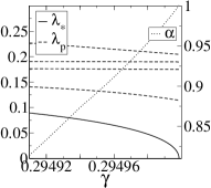
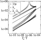
Figure 3: Left: relative participation of the lowest normal mode in the non-affine elastic displacement field, $\alpha^{*}\doteq\left(\xi^{*}/\lambda^{*}\right)^{2}/\sum_{p}\left(\xi_{p}/\lambda_{p}\right)^{2}$ (dotted); lowest eigenvalue of the dynamical matrix (solid); next several eigenvalues (dashed). b) In log-log scale (as a guide to the eye, the thick black line is $\sqrt{\gamma_{c}-\gamma}$): $1/\mu$ (circles); lowest eigenvalue (squares); next several eigenvalues minus their terminal values (diamonds).

In order to understand more specifically how the elastic constants behave close to $\gamma_{c}$, let us consider the functions $\lambda_{p}(\gamma)$, which are continuous on a small interval close to $\gamma_{c}$ (the second derivatives of the potential are supposed to be regular). Close to the yield point, $\gamma_{c}$, the deformation is dominated by the lowest normal mode: $\mathring{\bf\vec{r}}(\gamma)-\mathring{\bf\vec{r}}(\gamma_{c})\sim x(\gamma)\,{\bf\vec{\Psi}}^{*}(\gamma_{c})$ . (We project the deformation on the mode ${\bf\vec{\Psi}}^{*}$ at the yield point.) From this relation and (5), we obtain the dominant contribution: ${\rm d}x/{\rm d}\gamma\sim-\xi^{*}(\gamma_{c})/\lambda^{*}(\gamma)$. The coordinate $x$ measures a true displacement in configuration space: we expect that no singular behavior occurs in this rescaled coordinate whence, $\lambda^{*}(x)$ should vanish regularly, $\lambda^{*}(x)\sim ax$ close to $x=0$. From this assumption, it results: $x(\gamma)\sim\sqrt{2\xi^{*}(\gamma_{c})(\gamma_{c}-\gamma)/a}$. This relation controls entirely the behavior of all observables when approaching the yield point: any observable $A$ which behaves regularly as a function of $x$ (any regular function of molecular configurations) “accelerates” close to the yield point: ${\rm d}A/{\rm d}\gamma\sim 1/\sqrt{\gamma_{c}-\gamma}$. In particular, we obtain, ${\rm d}\mathring{\bf\vec{r}}/{\rm d}\gamma\sim{\bf\vec{\Psi}}_{p}/\sqrt{\gamma_{c}-\gamma}$, and $\lambda^{*}(\gamma)=\sqrt{2a\xi^{*}(\gamma_{c}-\gamma)}$, whence, $\widetilde{\mu}\sim-(\xi^{*})^{3/2}/\sqrt{2a(\gamma_{c}-\gamma)}$. We could observe these scalings numerically by a careful approach to the yield point, as shown figure 3. A similar divergence is observed for the compression modulus, but with a different prefactor, determined by the normal mode decomposition of the ${\bf\vec{\Xi}}$ field associated with pure compression.

Figure 4: Left: Non-affine elastic displacement field at a distance $\gamma_{c}-\gamma\sim 10^{-10}$ from the transition. Note the quadrupolar alignment with the direction of applied strain. Right: The local relative displacement field (the displacement of each particle measured with respect to the average displacement of its neighbors) which is incurred after the entire plastic cascade. The solid line is a guide to the eye oriented along the oblique Bravais axis.

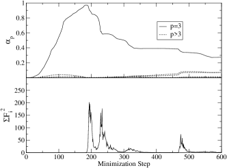
Figure 5: Evolution of the displacement field during the irreversible cascade corresponding to the event circled in figure 1. Top: contribution $\alpha^{*}$ (solid line) of the critical mode and $\alpha_{p}(t)$ (dashed line) of the next five modes to the displacement field. Bottom: sum of the squares of the forces on the particles.

We now turn to the overall plastic event following failure (see figure 4 and 5). We have already shown, in similar atomistic systems, that any single plastic event involves a cascade of local rearrangements. MaloneyL04 Our preceding work suggested that the overall plastic event was controlled by long range elastic interactions and differed from the displacement fields which dominate the onset of failure. Our present normal mode decomposition allows us to gain more insight into this process. Writing $\mathring{\bf\vec{r}}(t)-\mathring{\bf\vec{r}}(0)=\sum_{p}\Delta\xi_{p}(t)\,{\bf\vec{\Psi}}_{p}(\gamma_{c})$, we extract the quantities $\alpha_{p}\doteq(\Delta\xi_{p}(t))^{2}/\sum_{p}(\Delta\xi_{p}(t))^{2}$, which are shown figure 5 for the lowest frequency modes. To trigger the relaxation, we shear the system forward by a small amount of shear, $\gamma-\gamma_{c}\sim 10^{-5}$. The initial affine displacement serves as a perturbation and projects randomly on the normal modes, whence the contributions $\alpha_{p}$ start around zero. We observe that (i) the initiation of the cascade is clearly dominated by the critical mode (ii) this effect suddenly stops before reaching the first peak in $\sum_{i}F_{i}^{2}$ (this peak correspond to the first inflection point of energy vs. minimization step) (iii) the subsequent displacement appears to be random, when projected on the lowest part of the spectrum, indicating that low frequency normal modes are irrelevant for the latter stages of plastic failure. The system escapes its initial inherent structure in the direction of the lowest normal mode, whereas, in the late stages of a plastic event the emergence of long-range elastic interactions supersedes the low energy modes responsible for the onset of failure.

To conclude, we wish to stress that we expect our analysis to apply to many materials, to modes of deformation other than uniform shear, and to several experimental protocols at the nanoscale, including nanoindentation studies. Knowing the detailed behavior of elastic constants at incipient plasticity opens the route toward a possible control of material deformation at the nanometer scale.

This work was partially supported under the auspices of the U.S. Department of Energy by the University of California, Lawrence Livermore National Laboratory under Contract No. W-7405-Eng-48, by the NSF under grants DMR00-80034 and DMR-9813752, by the W. M. Keck Foundation, and EPRI/DoD through the Program on Interactive Complex Networks. CM would like to acknowledge the guidance and support of V. V. Bulatov and J. S. Langer and the hospitality of LLNL University Relations.

References

- (1) C. A. Schuh and T. G. Nieh, Acta Mater. 51, 87 (2003).
- (2) B. Miller, C. OHern, and R. P. Behringer, Phys. Rev. Lett. 77, 3110 (1996).
- (3) E. Pratt and M. Dennin, Phys. Rev. E 67, 051402 (2003).
- (4) K. Maeda and S. Takeuchi, J Phys-F-Metal Phys 8, L283 (1978).
- (5) D. L. Malandro and D. J. Lacks, J. Chem. Phys. 110, 4593 (1999).
- (6) A. Tanguy, J. P. Wittmer, F. Leonforte, and J.-L. Barrat, Phys. Rev. B 66, 174205 (2002).
- (7) C. Maloney and A. Lemaître, cond-mat/0402148 .
- (8) J. Li et al., Nature 418, 307 (2003).
- (9) R. Hill, J. Mech. Phys. Sol. 10, 1 (1962).
- (10) D. Wallace, Thermodynamics of Crystals (Wiley, New York, 1972).
- (11) J. F. Lutsko, J. Appl. Phys. 64, 1152 (1988).
- (12) J. Ray and A. Rahman, J. Chem. Phys. 80, 4423 (1984).
- (13) J. R. Ray, M. C. Moody and A. Rahman, Phys. Rev. B 32, 733 (1985).
- (14) T. Barron and M. Klein, proc. Phys. Soc. 85, 523 (1965).