Construction and properties of assortative random networks

Abstract

Many social networks exhibit assortative mixing so that the predictions of uncorrelated models might be inadequate. To analyze the role of assortativity we introduce an algorithm which changes correlations in a network and produces assortative mixing to a desired degree. This degree is governed by one parameter $p$. Changing this parameter one can construct networks ranging from fully random ($p=0$) to totally assortative ($p=1$). We apply the algorithm to a Barabási-Albert scale-free network and show that the degree of assortativity is an important parameter governing geometrical and transport properties of networks. Thus, the diameter of the network and the clustering coefficient increase dramatically with the degree of assortativity. Moreover, the concentration dependences of the size of the giant component in the node percolation problem for uncorrelated and assortative networks are strongly different.

PACS numbers: 05.50.+q, 89.75.Hc

Introduction

Complex networks have recently attracted a burst of interest as an indispensable tool of description of different complex systems. Thus, technological webs as the Internet and the World Wide Web, as well as other natural and social systems like intricate chemical reactions in the living cell, the networks of scientific and movie actors’ collaborations, and even human sexual contacts have been successfully described through scale-free networks, networks with the degree distribution $P(k)\sim k^{-\gamma}$ [1, 2]. The degree distribution $P(k)$ is one of the essential measures used to capture the structure of a network, and gives the probability that a node chosen at random is connected with exactly $k$ other vertices of the network.

Recently, it was pointed out that the existence of degree correlations among nodes is an important property of the real networks [3, 4, 5, 6, 7, 8, 9, 10, 11, 12, 13, 14, 15]. Thus, many social networks show that nodes having many connections tend to be connect with other highly connected nodes [4, 6]. In the literature this characteristics is usually dented as assortativity, or assortative mixing. On the other hand, technological and biological networks often have the property that nodes with high degree are preferably connected with ones with low degree, a property referred to as dissortativity [3, 7]. Such correlations have an important influence on the topology of networks, and therefore they are essential for the description of spreading phenomena, like spreading of information or infections, as well as for the robustness of networks against intentional attack or random breakdown of their elements [16, 17, 18, 19, 20, 21].

In order to assess the role of correlations, especially of the assortative mixing, several studies have proposed procedures to build correlated networks [3, 23, 24, 25]. The most general of them are the ones proposed by Newman [3], and by Boguñá and Pastor-Satorras [25], who suggest two different ways to construct general correlated networks with prescribed correlations. Following the same goal, we however adopt a different perspective in this paper. We propose a simple algorithm producing assortative mixing, in which, instead of putting correlations by hand, we only try impose the intuitive condition that “nodes with similar degree connects preferably”. We then investigate the correlations which come out of our simple model. Thus, we present an algorithm, governed by the only parameter $p$, capable to generate assortative correlations to a desired degree. In order to study the effect of the assortative mixing, we apply our algorithm to a Barabási-Albert scale-free network [26], the one leading to the degree distribution $P(k)\sim k^{-3}$, and investigate the properties of the emerging networks in some detail.

The algorithm

In what follows we treat undirected networks. Starting from a given network, at each step two links of the network are chosen at random, so that the four nodes, in general, with different degrees, connected through the links two by two are considered. The step of our algorithm looks as follows. The four nodes are ordered with respect to their degrees. Then, with probability $p$, the links are rewired in a such a way that one link connects the two nodes with the smaller degrees and the other connects the two nodes with the larger degrees, otherwise the links are randomly rewired (Maslov-Sneppen algorithm [11]). In the case when one, or both, of these new links already existed in the network, the step is discarded and a new pair of edges is selected. This restriction prevents the appearance of multiple edges connecting the same pair of nodes. A repeated application of the rewiring step leads to an assortative version of the original network. Note that the algorithm does not change the degree of the nodes involved and thus the overall degree distribution in the network. Changing the parameter $p$, it is possible to construct networks with different degree of assortativity.

Correlations and assortativity

Let ${\cal E}_{ij}$ be the probability that a randomly selected edge of the network connects two nodes, one with degree $i$ and another with degree $j$. The probabilities ${\cal E}_{ij}$ determine the correlations of the network. We say that a network is uncorrelated when

$${\cal E}_{ij}=(2-\delta_{ij})\frac{iP(i)}{\langle i\rangle}\frac{jP(j)}{\langle j\rangle}:={\cal E}^{r}_{ij}\ \ \ ,$$ (1)

i.e, when the probability that a link is connected to a node with a certain degree is independent from the degree of the attached node. Here $\langle i\rangle=\langle j\rangle$ denotes the first moment of the degree distribution.

Assortativity means that highly connected nodes tend to be connected to each other with a higher probability than in an uncorrelated network. Moreover, the nodes with similar degrees tend to be connected with larger probability than in the uncorrelated case, i. e., ${\cal E}_{ii}>{\cal E}^{r}_{ii}$  $\forall i$. The degree of assortativity of a network can thus be characterized by the quantity [3]:

$${\cal A}=\frac{\sum_{i}{\cal E}_{ii}-\sum_{i}{\cal E}^{r}_{ii}}{1-\sum_{i}{\cal E}^{r}_{ii}}\ \ \ ,$$ (2)

which takes the value $0$ when the network is uncorrelated and the value $1$ when the network is totally assortative. (Note that finite-size effects and the constraint that no vertices are connected by more than one edge bound ${\cal A}$ from above by the values lower than 1 [22]).

Now, starting from the algorithm generator, we can obtain a theoretical expression for ${\cal E}_{ij}$ as a function of $p$. Let $E_{ij}$ be the number of links in the network connecting two nodes, one with degree $i$ and another with degree $j$, so that ${\cal E}_{ij}=E_{ij}/L$, where $L$ is the total number of links of the network. (Since undirected networks satisfy $E_{ij}=E_{ji}$, the restriction $i\leq j$ can be imposed without loss of generality). We now define the variable

$$F_{ln}=\sum^{n}_{r=l}\sum^{n}_{s=r}E_{rs}\ \ \ \ \ r\leq s\ \ ;\ \ l\leq n\ \ \ .$$ (3)

A careful analysis of the algorithm reveals that, every time the rewiring process is applied, $F_{ln}$ either does not change, or changes increasing or decreasing by unity. We can then calculated the probabilities that it changes, i. e., that $F_{ln}\rightarrow F_{ln}+1$ or $F_{ln}\rightarrow F_{ln}-1$. Here, the effect of multiple edges can be disregarded since they are rare in the thermodynamical limit of infinite networks. Taking into account all corresponding possibilities, we obtain for the probabilities of changes the following expressions:

$\displaystyle\left(X_{ln}-f_{ln}\right)^{2}+p\left(X_{ln}-f_{1n}+f_{1,l-1}\right)^{2}$

for $F_{ln}\rightarrow F_{ln}+1$ and

$\displaystyle f_{ln}\left[(1-p)(1-2X_{ln})+p(X_{1,l-1}-f_{1,l-1}-f_{1n})+f_{ln}\right]$

for $F_{ln}\rightarrow F_{ln}-1$. Here $f_{ln}=F_{ln}/L$, and $X_{ln}$ is given by:

$\displaystyle X_{ln}=\frac{1}{\langle k\rangle}\sum^{n}_{k=l}kP(k)\ \ \ \ \ \ \ \ \ \ \ \ l\leq n\ \ \ .$

(Note that $X_{ln}$ and $f_{ln}$ vanish when one of the indices is smaller than $1$, the minimal tolerated degree). Using this, we can calculate the expected value for $f_{ln}$. The process of repeated applying our algorithm corresponds to an ergodic Markov chain, and the stationary solution in the thermodynamical limit is given by the condition:

$$\left(X_{ln}-f_{ln}\right)^{2}+p\left(X_{ln}-f_{1n}+f_{1,l-1}\right)^{2}=$$ (4)

$\displaystyle f_{ln}\left[(1-p)(1-2X_{ln})+p(X_{1,l-1}-f_{1,l-1}-f_{1n})+f_{ln}\right]$

for all $l>1$. For $l=1$ this condition reduces to

$$(1+p)\left(X_{1n}-f_{1n}\right)^{2}=(1-p)f_{1n}\left[1-2X_{1n}+f_{1n}\right]\ .$$ (5)

Using Eq. (4) and Eq. (5) we can calculate $f_{ln}$. The solutions reads

$\displaystyle f_{ln}=\displaystyle{\frac{X^{2}_{ln}+\left(B_{n}-B_{n-1}\right)^{2}}{(1-p)/2+pX_{ln}+B_{n}+B_{n-1}}}\ \ \ \ \ \ \ l\leq n$

with

$\displaystyle B_{n}=\sqrt{\left[pX_{1n}+\frac{1-p}{4}\right]^{2}-pX^{2}_{1n}\left(\frac{1+p}{2}\right)}\ \ \ .$

Applying the definition, Eq.(3), we obtain the correlations:

$${\cal E}_{ij}=f_{ij}-f_{i,j-1}-f_{i+1,j}+f_{i+1,j-1}.$$ (6)

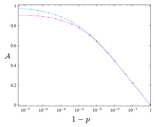
FIG. 1.: The lower curve corresponds to the measured assortativity ${\cal A}$ of our simulations, whereas the upper curve corresponds to the theory. We note that both curves coincide for ${\cal A}<0.7$. Above this value the finite-size corrections get important, leading to the measured value of ${\cal A}<1$ for $p\to 1$.

Finally, note that Eq.(6) reduces to the corresponding uncorrelated case ${\cal E}^{r}_{ij}$ when $p=0$, and reduces to

$${\cal E}_{ij}=\delta_{ij}\frac{iP(i)}{\langle i\rangle}$$ (7)

for the case $p=1$.

Simulation results

In our simulations we apply our algorithm to the Barabási-Albert network [26] with $N=10^{5}$ nodes and $L=2\cdot 10^{5}$ links. We measure ${\cal E}_{ij}$ as functions of $p$, and use them to calculate the corresponding values of ${\cal A}$. All simulation results are averaged over ten independent realizations of the algorithm as applied to the original network.

Fig. 1 shows the relation between the parameter $p$ and the coefficient of assortativity ${\cal A}$. The lower curve corresponds to the measured assortativity, and the upper to our theoretical prediction. Both curves coincide for ${\cal A}<0.7$. However, whereas the theoretical curve reach the value $1$ for $p\to 1$, the measured assortativity increases until the maximal value smaller than one (${\cal A}\to 0.913$) is reached. This was theoretically expected, and is due to the finite-size effects mentioned above.

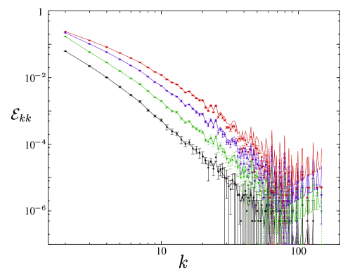
FIG. 2.: ${\cal E}_{kk}$ as a function of $k$ for different values of ${\cal A}$. From bottom to top: ${\cal A}=0$, $0.221$, $0.443$, and $0.640$. The points are the results of the simulations and the curves correspond to the theory.

To assess the goodness of the Eq. (6) we compare in the Fig. 2 the theoretical values of ${\cal E}_{kk}$, given by Eq. (6), with the simulations. The points correspond to the simulations and the curves are the corresponding theoretical results obtained based on the actual degree distribution of a particular realization of the network discussed. We note that the agreement is really excellent.

Diameter.— The diameter of a network is the average distance between every pair of vertices of the network, being defined as the number of edges along the shortest path connecting them. Uncorrelated scale-free networks show a very small diameter, typically growing as the logarithm of the network’s size. For networks with $N\simeq 10^{5}$ the diameter is about $d\simeq 6$. The results of the simulations show that the diameter grows rapidly when the assortativity of the network increases (fig. 3), so that it becomes hundred times larger than for the uncorrelated network when the coefficient of assortativity tend to its maximal value. In the inset we plot the diameter as a function of ${\cal K}-{\cal A}$, where ${\cal K}=0.913$ corresponds to this maximal value of ${\cal A}$ attainable in the network. For our particular Barabási-Albert network we thus have $d\propto(0.913-{\cal A})^{-1.12}$.

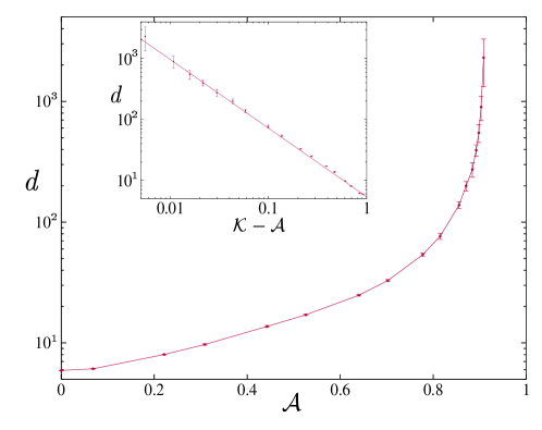
FIG. 3.: Diameter of the network versus coefficient of assortativity. We note that the diameter grows rapidly when ${\cal A}$ increases. In the inset the diameter is plotted on double logarithmic scales as function of ${\cal K}-{\cal A}$, being ${\cal K}=0.931$. The slope of the straight line is 1.12.

Clustering coefficient.— Clustering coefficients of a network are a measure of the number of loops (closed paths) of length three. The notion has its roots in sociology, where it was important to analyze the groups of acquaintances in which every member knows every other one. To discuss the concept of clustering, let us focus first on a vertex, having $k$ edges connected to $k$ other nodes termed as nearest neighbors. If these nearest neighbors of the selected node were forming a fully connected cluster of vertices, there would be $k(k-1)/2$ edges between them. The ratio between the number of edges that really exist between these $k$ vertices and the maximal number $k(k-1)/2$ gives the value of the clustering coefficient of the selected node. The clustering coefficient of the whole network $C$ is then defined as the average of the clustering coefficients of all vertices. One can also speak about the clustering coefficient of nodes with a given degree $k$, referring to the average of the clustering coefficients only over this type of nodes. We shall denote this degree-dependent clustering coefficient by $\bar{C}(k)$, to distinguish it from $C$.

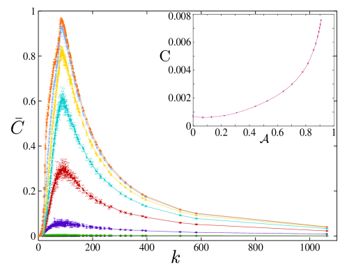
FIG. 4.: $\bar{C}(k)$ as a function of the degree of nodes $k$. Different curves correspond to different values of ${\cal A}$. From bottom to top ${\cal A}=0$, $0.069$, $0.221$, $0.443$, $0.640$, $0.777$, $0.856$, and $1$. Inset: clustering coefficient $C$ versus the degree of assortativity ${\cal A}$.

Fig. 4 shows the variation of both clustering coefficients with the assortativity of the network. The clustering coefficient $C$ increases with the assortativity (inset of the figure). The variation of $\bar{C}(k)$ shows more interesting features. The simulations show a peak around $k=90$ (probably a finite size effect) whose height increases with the assortativity of the network. In the uncorrelated case $\bar{C}(k)$ does not depend on $k$ [13], but a strong tendency to clustering (for relatively large $k$) emerges when ${\cal A}$ grows. We also observe in our simulations that $\bar{C}(k=2)=0$ when ${\cal A}\simeq 1$ ($k=2$ correspond to the minimal degree of our vertices). This is not surprising since in a strongly assortative case almost all nodes with degree $k=2$ are connected between themselves, forming one or several large loops of length larger than three. This means that all nodes having this minimal degree (in our simulations the half of the total number of vertices) do not tend to contribute to the clustering coefficient $C$.

In the present contribution we concentrate on the investigation of the properties of the proposed algorithm. However, we suggest, in relation to real networks, a simple modification of the algorithm, that perhaps could be useful. Thus, in order to generate assortativity only among highly connected vertices, one can apply the algorithm above only when at least one of the four nodes selected at the corresponding step has a degree larger than some chosen $k$. Provided all four nodes have a smaller degree, the the Maslov-Sneppen step is used. This procedure could lead to a larger value for the clustering coefficient, as it is observed in real networks ($C\geq 0.1$) [1]. The last ones might, however, have a much more intricate structure, partly governed by the metrics of the underlying space, as in the models discussed in [27], so that caution has to be exercised when applying results of theoretical models disregarding metrical relations to real networks.

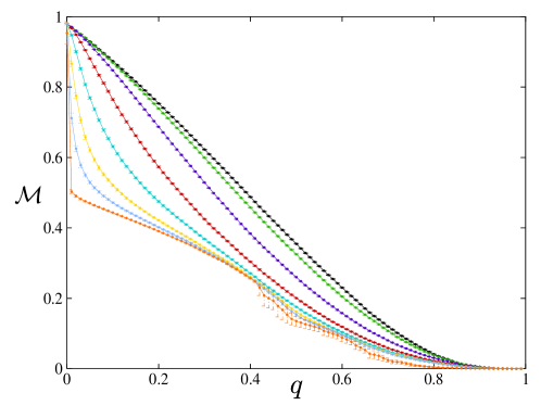
FIG. 5.: Fraction of nodes ${\cal M}$ in the giant component depending on the fraction of nodes removed from the network. The graph compares the results for different degrees of assortativity. From top to bottom: ${\cal A}=0$, $0.069$, $0.221$, $0.443$, $0.640$, $0.777$, $0.856$, and $1$.

Node percolation.— Node percolation corresponds to removal of a certain fraction of vertices from the network, and is relevant when discussing their vulnerability to a random attack. Let $q$ be the fraction of the nodes removed. At a critical fraction $q_{c}$, the giant component (largest connected cluster) breaks into tiny isolated clusters. Fig. 5 shows the fraction of nodes ${\cal M}$ in the giant component as a function of $q$ for different degrees of assortativity of the network. We note that the behavior of ${\cal M}(q)$ changes gradually with ${\cal A}$ from the uncorrelated case (upper curve) to a quite different behavior when ${\cal A}\rightarrow 1$ (lower curve), which indicates a very different topology in the network when it is strongly assortative. However, although the particular form of the ${\cal M}$ dependence is different for different degrees of assortativity, the absence of the transition at finite concentrations ($q_{c}=1$) and the overall type of the critical behavior for correlated networks with the same $P(k)$ seems to be the same as for uncorrelated networks, namely the one discussed in Refs. [28, 29]. We also point out that in case ${\cal A}\simeq 1$, a finite network is no longer fully connected: part of the nodes does not belong to the giant component even for $q=0$. The results suggest that, in the thermodynamical limit, the giant cluster at $q=0$ contains around a half of all nodes, and that its density then decays smoothly with $q$.

Conclusions

In summary, we present an algorithm to generate assortatively correlated networks. In the termodynamical limit we obtain a theoretical expression for the generated correlations, which only depends on the degree distribution of the network and on the turnable parameter $p$ of the algorithm. Finally, we show that assortative correlations have a drastic influence on the statistical properties of networks, changing strikingly their diameter and clustering coefficient, as well as their percolation properties.

We also indicate that with a minor change in our algorithm one can produces dissortative mixing too. The only change would be the following: after ordering the nodes with respect to their degree, one rewires, with probability $p$, the edges so that one link connects the highest connected node with the node with the lowest degree and the other link connects the two remaining vertices; with probability $1-p$ one rewires the links randomly.

REFERENCES

- [1] R. Albert and A.-L. Barabási, Rev. Mod. Phys. 74, 47 (2002).
- [2] S.N. Dorogovtsev and J.F.F. Mendes, Adv. Phys. 51, 1079 (2002).
- [3] M. E. J. Newman, Phys. Rev. E 67, 026126 (2003).
- [4] M. E. J. Newman, Phys. Rev. Lett. 89, 208701 (2002).
- [5] A. Vázquez, M. Boguñá, Y. Moreno, R. Pastor-Satorras, and A. Vespignani, Phys. Rev. E 67, 046111 (2003).
- [6] A. Capocci, G. Caldarelli, and P. De Los Rios, Phys. Rev. E 68, 047101 (2003).
- [7] R. Pastor-Satorras, A. Vázquez, and A. Vespignani, Phys. Rev. Lett. 87, 258701 (2001).
- [8] M. E. J. Newman and J. Park, Phys. Rev. E 68, 036112 (2003).
- [9] J. Berg, and M. Lässig, Phys. Rev. Lett. 89, 228701 (2002).
- [10] K.-I. Goh, E. Oh, B.Kahng, and D. Kim, Phys. Rev. E 67, 017101 (2003).
- [11] S. Maslov, and K. Sneppen, Science 296 910 (2002).
- [12] P. L. Krapivsky, and S. Redner, Phys. Rev. E 63 066123 (2001).
- [13] S. N. Dorogovtsev, Phys. Rev. E 69, 027104 (2004).
- [14] D. S. Callaway, J. E. Hopcroft, J. M. Kleinberg, M. E. J. Newman, and S. H. Strogatz, Phys. Rev. E 64, 041902 (2001).
- [15] J. Park and M. E. J. Newman, Phys. Rev. E 68, 026112 (2003).
- [16] M. Boguñá, R. Pastor-Satorras, and A. Vespignani, Phys. Rev. Lett. 90, 028701 (2003).
- [17] V. M. Eguíluz, and K. Klemm, Phys. Rev. Lett. 89, 108701 (2002).
- [18] M. Boguñá, and R. Pastor-Satorras, Phys. Rev. E 66, 047104 (2002).
- [19] N. Schwartz, R. Cohen, D. ben-Avraham, A.-L. Barabási, and S. Havlin, Phys. Rev. E 66, 015104 (2002).
- [20] A. Vázquez, and Y. Moreno, Phys. Rev. E 67, 015101 (2003).
- [21] Y. Moreno, J. B. Gómez, and A. F. Pacheco, Phys. Rev. E 68, 035103 (2003).
- [22] S. Maslov, K. Sneppen, and A. Zaliznyak, Physica A 333, 529 (2004).
- [23] A. Ramezanpour, V. Karimipour, and A. Mashaghi, Phys. Rev. E 67, 046107 (2003).
- [24] R. Xulvi-Brunet, W. Pietsch, and I. M. Sokolov, Phys. Rev. E 68, 036119 (2003).
- [25] M. Boguñá and R. Pastor-Satorras, Phys. Rev. E 68, 036112 (2003).
- [26] A.-L. Barabási, and R. Albert, Science 286, 509 (1999).
- [27] L.M. Sander, C.P. Warren, and I.M. Sokolov, Phys. Rev. E 66, 056105 (2002).
- [28] R. Cohen, K. Erez, D. ben-Avraham, and S. Havlin, Phys. Rev. Lett. 85, 4626 (2000).
- [29] R. Cohen, D. ben-Avraham, and S. Havlin, Phys. Rev. E 66, 036113 (2002).