Circling particles and drafting in optical vortices

Abstract

Particles suspended in a viscous fluid circle in optical vortices generated by holographic optical-tweezer techniques [Curtis J E and Grier D G 2003 Phys. Rev. Lett. 90 133901]. We model this system and show that hydrodynamic interactions between the circling particles determine their collective motion. We perform a linear-stability analysis to investigate the stability of regular particle clusters and illustrate the limit cycle to which the unstable modes converge. We clarify that drafting of particle doublets is essential for the understanding of the limit cycle.

1 Introduction

Hydrodynamic interactions occur between particles or bodies whenever they move relative to each other in a viscous fluid. Due to their long-range nature, they are important for the dynamic properties of colloidal suspensions exemplified by the self- and collective diffusion [1, 2, 3, 4], sedimentation [5, 6, 7], or the aggregation of particles [8]. Through the correlated motion of a pair of colloids trapped in optical tweezers, one can directly measure the effect of hydrodynamic interactions [9, 10, 11, 12]. Furthermore, hydrodynamic interactions give rise to interesting collective behavior, e.g., periodic or almost periodic motions in time [13, 14] or even transient chaotic dynamics in the sedimentation of particles [15]. And they lead to pattern formation of rotating motors [16] with a possible 2D melting transition of biological motors like ATP-synthase embedded in a membrane [17]. Hydrodynamic interactions are treated in the low-Reynolds-number regime which is also relevant for biology. It determines the problem of how microorganisms move forward [18]. Certain bacteria accomplish this, e.g., by cranking helical flexible rods [19]. In addition, recent experiments show that laminar flows initiate the asymmetries between the right- and left-hand side of the body at an early stage of the embryonic development [20, 21, 22].

The work presented here is motivated by experiments of Curtis and Grier [23]. They created toroidal optical traps known as optical vortices with the help of holographic techniques. In the bright circumference of an optical vortex, they could trap particles which circulated around the ring due to scattering forces which result from the orbital angular momentum of light. In this article, we model the system of circling particles. We demonstrate that hydrodynamic interactions determine their interesting collective motion which we analyze by methods used in the study of non-linear dynamics. In particular, we identify a limit cycle which is governed by drafting of particle doublets.

The outline of the article is as follows. In section 2, we first define our model system of particles moving in a ring-like trap and summarize the basic equations for the description of the dynamics. The stability of regular $N$-particle clusters in the ring is investigated in section 3 by means of a linear stability analysis. Section 4 then describes the nonlinear dynamics of perturbed clusters. We introduce the periodic limit cycle of the three-particle system and perform a harmonic analysis. The influence of the trap strength on the dynamics is discussed. Furthermore, we briefly address the dynamics in fairly weak traps. Finally, in section 5, we present the particle velocities as a function of ring radius and particle number.

2 Modelling particle dynamics in a toroidal optical trap

We consider non-Brownian, equal-sized spherical particles suspended in a viscous fluid in the regime of low Reynolds numbers whose mutual interactions are solely of hydrodynamic origin. We mimick the basic features of particles captured in an optical vortex by applying a constant tangential force $F^{\phi}$ to each particle and by keeping the particles on a ring of radius $R$ by means of a harmonic radial trap with force constant $K^{r}$ (figure 1). The particle motion is effectively two-dimensional in the plane of the ring ($z=0$); thus, the particle positions are best described by polar coordinates, $r_{i}$ and $\phi_{i}$. With the radial and tangential unit vectors at the position of particle $i$, $\boldsymbol{e}_{i}^{r}=(\cos\phi_{i},\sin\phi_{i},0)$ and $\boldsymbol{e}_{i}^{\phi}=(-\sin\phi_{i},\cos\phi_{i},0)$, the total external force acting on particle $i$ then reads

$$\boldsymbol{F}_{i}=F^{\phi}\boldsymbol{e}_{i}^{\phi}-K^{r}(r_{i}-R)\boldsymbol{e}_{i}^{r}\,.$$ (1)

• 

Figure 1: Definition of our model system of an optical vortex. The particles are driven by a constant tangential force and trapped in the ring by a harmonic radial force. In order to avoid overlaps, the particles repel each other at very short distances.

Note that the assumption of a constant tangential driving force $F^{\phi}$ is a rough approximation since the intensity profile of an optical vortex is modulated along the ring as described by the topological charge $\ell$ of the vortex [23]. However, if $\ell$ is large so that the period of the modulations is small compared to the particle size, then our approximation seems to be reasonable.

In order to prevent that particles overlap in the simulations, we add a repulsive interaction which becomes relevant only when two particles are very close to each other. We use a hard-sphere-type interaction potential where a “hard core” with diameter $2a$ is surrounded by a “soft” repulsive potential (figure 1) [28]:

$$V^{\rm rep}(r_{ij})=W\left[\left(\frac{r_{ij}}{2a}\right)^{m}-1\right]^{-1}\,.$$ (2)

Here, $r_{ij}$ is the center-to-center distance between particles $i$ and $j$, and $a$ is the particle radius. This choice is primarily due to numerical reasons, but can nevertheless be justified from the physical point of view since even hard-sphere-like colloids show a “soft” repulsive potential at very short distances [28]. We choose the commonly used Lennard-Jones exponent $m=12$ so that the repulsion only acts at very short distances, and we tune the prefactor $W$ such that the minimal inter-particle gap $r_{ij}-2a$ in the simulations is of the order of $10^{-4}a$.

In the regime of low Reynolds numbers, the flow of an incompressible fluid with viscosity $\eta$ obeys the Stokes or creeping flow equations [24, 25, 2]

$$\eta\nabla^{2}\boldsymbol{u}-\nabla p=\boldsymbol{0}\,,\quad\nabla\cdot\boldsymbol{u}=0\,,$$ (3)

where $\boldsymbol{u}$ is the flow field and $p$ the hydrodynamic pressure. Imposing stick boundary conditions on the surfaces of all particles suspended in the fluid, the motions of the particles are mutually coupled via the flow field. Due to the linearity of (3), the translational and rotational velocities of the particles, $\boldsymbol{v}_{i}$ and $\boldsymbol{\omega}_{i}$ ($i=1,\ldots,N$), depend linearly on all external forces and torques acting on the particles, $\boldsymbol{F}_{j}$ and $\boldsymbol{T}_{j}$ [24, 25, 2]:

$$\boldsymbol{v}_{i}=\sum\limits_{j=1}^{N}\left(\boldsymbol{\mu}^{\rm tt}_{ij}\boldsymbol{F}_{j}+\boldsymbol{\mu}^{\rm tr}_{ij}\boldsymbol{T}_{j}\right)\,,\quad\boldsymbol{\omega}_{i}=\sum\limits_{j=1}^{N}\left(\boldsymbol{\mu}^{\rm rt}_{ij}\boldsymbol{F}_{j}+\boldsymbol{\mu}^{\rm rr}_{ij}\boldsymbol{T}_{j}\right)\,.$$ (4)

The central quantities are the $3\times 3$ mobility tensors $\boldsymbol{\mu}^{\rm tt}_{ij}$, $\boldsymbol{\mu}^{\rm rr}_{ij}$, $\boldsymbol{\mu}^{\rm tr}_{ij}$, and $\boldsymbol{\mu}^{\rm rt}_{ij}$. They depend on the current spatial configuration of all particles, i.e., the set of position vectors $\{\boldsymbol{r}_{1},\ldots,\boldsymbol{r}_{N}\}$ in the case of spherical shape.

As there are no external torques in our model, i.e., $\boldsymbol{T}_{j}\equiv\boldsymbol{0}$, and as we are not interested in the rotational motion of the particles, the remaining equation of motion for our problem is

$$\dot{\boldsymbol{r}}_{i}\equiv\boldsymbol{v}_{i}=\sum\limits_{j=1}^{N}\boldsymbol{\mu}^{\rm tt}_{ij}\boldsymbol{F}_{j}\,.$$ (5)

Since the mobility tensors $\boldsymbol{\mu}^{\rm tt}_{ij}$ are nonlinear functions of all particle positions $\{\boldsymbol{r}_{k}\}$, (5) describes the coupled nonlinear dynamics of $N$ particles.

The first-order approximation (with respect to inverse particle distances $r_{ij}$) for the mobilities of particles moving in an unbounded and otherwise quiescent fluid is the well-known Oseen tensor [2]

$$\boldsymbol{\mu}^{\rm tt}_{ij}=\frac{3\mu^{\rm t}a}{4r_{ij}}\,\bigg{(}\boldsymbol{1}+\frac{\boldsymbol{r}_{ij}\otimes\boldsymbol{r}_{ij}}{r_{ij}^{2}}\bigg{)}\,,$$ (6)

where $\mu^{\rm t}=(6\pi\eta a)^{-1}$ is the Stokes mobility for a translating sphere; the self-mobilities are $\boldsymbol{\mu}^{\rm tt}_{ii}=\mu^{\rm t}\boldsymbol{1}$. All the other mobility tensors in (4) vanish in this approximation. Note that the Oseen tensor is the Green function of the Stokes equations (3), i.e., it considers pointlike particles and hence does not include rotational couplings.

Higher order approximations of all mobility tensors can be calculated, e.g., via the multipole expansion method [26]. It has been implemented in the numerical library hydrolib [27], which we use in our simulations. For the numerical integration of the highly nonlinear equation of motion (5), we apply a fourth-order Runge-Kutta scheme. The time step is chosen such that the corresponding change in the angular position is of the order of $1^{\circ}$.

3 Stability analysis of regular clusters

In this section, we study the stability of regular $N$-particle clusters. By “regular” we mean configurations with $N$-fold symmetry, like the ones shown in figure 2. Due to this symmetry, all particle positions are equivalent, i.e., the angular velocity $\dot{\phi}_{i}$ has to be the same for all particles. The radial positions of the particles do not change either, which can also be justified by a simple symmetry argument. Let us start with a regular configuration where $r_{i}=R$ for all particles, so there is not radial force component in (1). Due to linearity, $\dot{r}_{i}\propto F^{\phi}$, which means that changing the direction of $F^{\phi}$ inverts the direction of $\dot{r}_{i}$. However, since there is no difference if the cluster rotates clockwise or counterclockwise, the radial velocity must be the same for both directions, i.e., $\dot{r}_{i}\equiv 0$ and $r_{i}\equiv R$. Therefore, a regular cluster remains unchanged and rotates with constant frequency $\Omega_{N}$.

• 

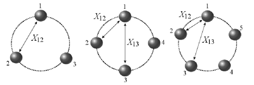
Figure 2: Regular $N$-particle clusters.

In regular clusters, the particles are well separated for sufficiently large radius $R$, and we may approximate the hydrodynamic interactions by the Oseen tensor (6). The particle positions of the regular clusters are given by $r_{i}=R$ and $\phi_{i}=\Phi_{i}(t)=(2\pi/N)i+\Omega_{N}t$. With $\boldsymbol{F}_{i}=F^{\phi}\boldsymbol{e}_{i}^{\phi}$, we derive from (5) the rotational frequency of an $N$-particle cluster,

$$\Omega_{N}=\Omega_{1}\bigg{[}1+\frac{3}{4}\sum\limits_{j\neq i}\frac{1}{X_{ij}}\,\frac{1+3\cos\Phi_{ij}}{2}\bigg{]}\,,\quad\Omega_{1}=\frac{\mu^{\rm t}F^{\phi}}{R}\,\,,$$ (7)

where $X_{ij}=\sqrt{2}(R/a)\sqrt{1-\cos\Phi_{ij}}$ and $\Phi_{ij}=(2\pi/N)(j-i)$ are the respective spatial and angular distances between particles $i$ and $j$.

To investigate the stability of these $N$-particle clusters against small radial and angular particle displacements, we introduce $r_{i}=R[1+\delta\rho_{i}(t)]$ and $\phi_{i}=\Phi_{i}(t)+\delta\phi_{i}(t)$. Using the forces (1) and the Oseen tensor (6), we linearize the equation of motion (5) in terms of the small perturbations $\delta\rho_{i}$ and $\delta\phi_{i}$:

$$\frac{\rmd}{\rmd\tau}\,\delta\rho_{i}(\tau)= -\mathcal{K}\,\delta\rho_{i}(\tau)$$

$$+\frac{3}{4}\,\sum\limits_{j\neq i}\bigg{[}\frac{1}{X_{ij}}\bigg{(}\frac{(5-3\cos\Phi_{ij})\sin\Phi_{ij}}{4(1-\cos\Phi_{ij})}+\mathcal{K}\,\frac{1-3\cos\Phi_{ij}}{2}\bigg{)}\delta\rho_{j}(\tau)\bigg{]}$$

$$-\frac{3}{4}\bigg{[}\sum\limits_{j\neq i}\frac{1}{X_{ij}}\,\frac{3(1-\cos\Phi_{ij})}{4}\bigg{]}\delta\phi_{i}(\tau)$$

$$+\frac{3}{4}\sum\limits_{j\neq i}\bigg{[}\frac{1}{X_{ij}}\,\frac{3(1-\cos\Phi_{ij})}{4}\,\delta\phi_{j}(\tau)\bigg{]}\,\,,$$

$$\frac{\rmd}{\rmd\tau}\,\delta\phi_{i}(\tau)= -\bigg{[}1+\frac{3}{4}\sum\limits_{j\neq i}\frac{1}{X_{ij}}\,\frac{3(1+3\cos\Phi_{ij})}{4}\bigg{]}\delta\rho_{i}(\tau)$$ (8)

$$-\frac{3}{4}\sum\limits_{j\neq i}\bigg{[}\frac{1}{X_{ij}}\bigg{(}\frac{1+3\cos\Phi_{ij}}{4}+\mathcal{K}\,\frac{3\sin\Phi_{ij}}{2}\bigg{)}\delta\rho_{j}(\tau)\bigg{]}$$

$$-\frac{3}{4}\sum\limits_{j\neq i}\bigg{[}\frac{1}{X_{ij}}\,\frac{(7-3\cos\Phi_{ij})\sin\Phi_{ij}}{4(1-\cos\Phi_{ij})}\,\delta\phi_{j}(\tau)\bigg{]}\,\,,$$

where $\tau=\Omega_{1}t$ is the reduced time, and the dimensionless parameter $\mathcal{K}=K^{r}R/F^{\phi}$ measures the strength of the radial trap relative to the tangential driving force. The corresponding eigenvalue problem was solved numerically by using the computer-algebra package maple. This analysis reveals that there are the following types of stable and unstable eigenmodes (depending on the number of particles) for the coupled displacements $(\delta\rho_{1}(\tau),\ldots,\delta\rho_{N}(\tau),\delta\phi_{1}(\tau),\ldots,\delta\phi_{N}(\tau))$: (i) a constant angular shift, (ii/iii) non-oscillating damped or unstable, and (iv/v) oscillating damped or unstable. Figure 3 shows an example of an unstable oscillating mode (type v). In table 1, we give the number of eigenmodes classified by their eigenvalues $\lambda$ for even and odd particle numbers.

• 

Figure 3: Representative example of the angular coordinate of an unstable oscillating mode (here: $N=4$, $R/a=10$, $\mathcal{K}=10$). The linear theory and the simulations agree very well up to amplitudes of several percent of $2\pi/N$. (Only every 100th data point from the simulation is plotted.)

• 	(i)	(ii)	(iii)	(iv)	(v)
  $N$	$\lambda=0$	$\lambda\in\mathbb{R}_{-}$	$\lambda\in\mathbb{R}_{+}$	Re $\lambda<0$	Re $\lambda>0$
  odd	1	1	—	$N-1$	$N-1$
  even	1	2	1	$N-2$	$N-2$

Table 1: Number of eigenmodes classified by their eigenvalues $\lambda$ for even and odd particle numbers $N$. $\mathbb{R}_{\pm}$ means a positive or negative real number. (i) constant angular shift, (ii/iii) non-oscillating damped or unstable modes, (iv/v) oscillating damped or unstable modes.

The occurence of stable and unstable modes can be compared to a saddle point in the framework of the analysis of dynamic systems. A cluster configuration with arbitrary small radial and angular displacements of the particles is practically unstable since contributions of unstable modes will grow, while stable modes will relax to zero.

For $N=3$, we have also determined the eigenvalues analytically by an expansion to first order in $a/R$:

$$\lambda_{1} =0 \mbox{(type i)}\,,$$

$$\lambda_{2} =-\mathcal{K}\bigg{(}1-\frac{\sqrt{3}}{10}\,\frac{a}{R}\bigg{)} \mbox{(type ii)}\,,$$

$$\lambda_{3,4} =-\mathcal{K}-\bigg{[}\bigg{(}\frac{\sqrt{3}}{20}+\frac{27\sqrt{3}}{32}\,\frac{1}{\mathcal{K}}\bigg{)}\pm\rmi\,\frac{13\sqrt{3}}{32}\,\bigg{]}\frac{a}{R}\qquad \mbox{(type iv)}\,,$$

$$\lambda_{5,6} =\bigg{(}\frac{27\sqrt{3}}{2}\,\frac{1}{\mathcal{K}}\pm\rmi\,\frac{17\sqrt{3}}{32}\,\bigg{)}\frac{a}{R} \mbox{(type v)}\,.$$

In this case, a non-oscillating unstable mode (type iii) does not exist; it only occurs for even $N$ (see table 1).

4 Nonlinear dynamics of perturbed clusters

The amplitude of an unstable mode grows up to a certain magnitude in agreement with the linear analysis, until the nonlinear dynamics takes over (see figure 3). The amplitudes saturate, and the system finally tends towards a periodic limit cycle with oscillating particle distances. In figure 4 we show an example of such a dynamic transition from an unstable linear mode to the periodic limit cycle by plotting the angular coordinate $\phi(t)$ relative to $\Omega_{N}t$ as a function of time. Note that $\Omega_{N}$ is the rotational frequency of the regular $N$-particle cluster introduced in (7).

The mean slope in each of the two regimes (linear mode and limit cycle) gives a well-defined mean orbital frequency $\langle\Omega\rangle$, which is $\Omega_{N}$ for the linear mode. Clearly, $\langle\Omega\rangle$ and therefore the mean velocity of the particles is increased by the transition to the limit cycle, which means that the mean drag force on the particles is reduced.

• 

Figure 4: Dynamic transition in the angular coordinate from an unstable linear mode to the periodic limit cycle for three particles ($R/a=10$). The main curve and the insets (a), (b), and (d) show the angle $\phi(t)$ relative to $\Omega_{N}t$ as a function of time. In the inset (c), $\phi(t)-\langle\Omega\rangle t$ is plotted. Plots (a)–(c) correspond to a stiffness of $\mathcal{K}=10$. For comparison with (b), the transition regime for $\mathcal{K}=100$ is shown in (d). The dashed lines in (b) and (d) indicate the limit cycles.

• 

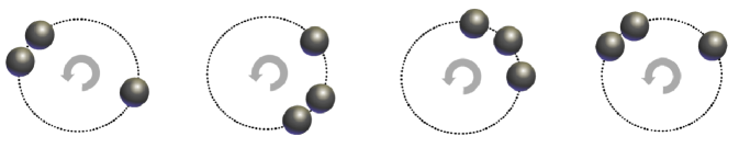
Figure 5: Basic mechanism of the periodic limit cycle. Two particles in close contact move faster than a single particle. When this pair reaches the third particle, they form an intermediate triplett, and finally, the first two particles escape as a new pair.

The character of the transition depends on the trap stiffness. It is quite sharp for weaker traps, where the transition takes place within a few oscillations, as shown in figure 4(b). For stronger traps, the mean frequency increases smoothly from the linear regime to the limit cycle, which is illustrated in figure 4(d). Furthermore, the onset of the transition is shifted to later times when the trap becomes stiffer.

Figure 5 introduces the basic mechanism underlying the periodic limit cycle. Two particles in close contact move faster than a single particle since the friction per particle is reduced due to the well-known effect of drafting. When such a pair reaches the third particle, they form a triplett for a short time. In this configuration, the mobility of the middle particle is larger since it is “screened” from the fluid flow by the outer particles. It therefore pushes the particle in front, so that the first two particles “escape” from the last one. The same principle also holds for more than three particles. In these cases, there can be more than one pair of particle.

For the limit cycle of three particles, we have performed a harmonic analysis using Fast Fourier Transformation. In order to separate the fast orbital dynamics of the particles (characterized by the mean angular frequency $\langle\Omega\rangle$) from their relative motions, we calculate the Fourier transform of $\phi(t)-\langle\Omega\rangle t=\sum_{\omega}[a(\omega)\cos\omega t+b(w)\sin\omega t]$. This yields the fingerprint of the dynamics relative to the mean circling velocity. In figure 6, we show the corresponding Fourier spectrum. Besides the characteristic frequency $\omega^{*}$ of the limit cycle, the higher harmonics $2\omega^{*}$ and $3\omega^{*}$ are also very pronounced.

• 

Figure 6: Fourier spectrum [$\cos$-coefficients $a(\omega)$ and $\sin$-coefficients $b(\omega)$] of the periodic limit cycle of three particles. Note that the frequencies $\omega$ are defined relative to the mean orbital frequency $\langle\Omega\rangle$.

• 

Figure 7: Characteristic frequency $\omega^{*}$ of the periodic limit cycle of three particles versus ring radius $R$. The different curves are related to different trap stiffnesses $K^{r}$.

The characteristic frequency $\omega^{*}$ decreases with increasing ring radius, as shown in figure 7, because it takes longer for a particle pair to reach the third particle on a larger ring. At constant ring radius, the characteristic frequency increases with the trap stiffness since particles in a stronger trap are better aligned along the ring, which makes the mechanism of the limit cycle more effective.

If the strength of the radial trap is decreased, the radial displacements of the particles increase so that they can pass each other. This happens at a reduced trap stiffness $\mathcal{K}=K^{r}R/F^{\phi}$ of the order of 1. For three particles and four particles, the limit cycle then consists of a compact triangular or rhombic-shaped cluster circling and rotating in the trap.

For four particles, we also find the limit cycle illustrated in figure 8. It occurs if the radial trap has medium strength so that compact particle clusters only have a finite life time. The first particle on the left is pushed in outward radial direction by the particles behind it and subsequently passed by the second particle. It, then, pushes the third one in inward radial direction, which in turn takes over the lead of the chain. Finally, the initial state is rebuild, where the first and the third particle are exchanged. Note that there is an intermediate state where the particles form a compact rhombic-shaped cluster, which, however, is not stable.

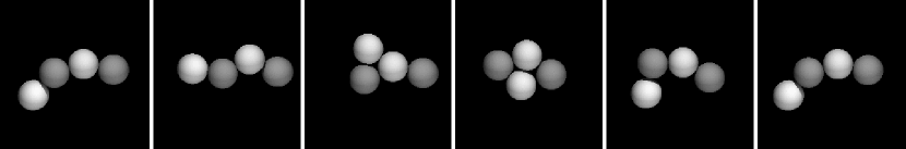
Figure 8: Dynamics of four particles in a weak radial trap. The motion shown is relative to the mean rotation along the ring trap. Only the relevant part of the ring is shown, the center of the ring is located at the bottom of the snapshots. The particles are running from right to left. During one cycle, the first and the third particle are exchanged. The particles are shaded differently in order to distinguish them.

5 Particle velocities

In figure 9 (left), we study the circling frequencies of regular clusters as a function of particle number $N$ for different ring radii $R$. At constant radius, the frequency increases with the number of particles since then the particles are closer together which reduces the drag. Note that for less than four particles, the frequency is reduced relative to the single particle value. Here, hydrodynamic interactions across the ring increase the drag on the particles. This effect is clearly more pronounced for small rings.

At constant particle distance $2\pi R/N$ or constant line density of the particles $N/(2\pi R)$, the drag is reduced when the ring radius increases [see figure 9 (right)]. This is due to the fact that in a ring with smaller curvature the particles are better “aligned” behind each other.

Figure 9: Circling frequencies of regular $N$-particle clusters, normalized to the frequency of a single sphere, as obtained from simulations. The two plots show the same data, left: as a function of particle number, right: as a function of particle line density. The arrow gives the direction of increasing ring radius.

• 

Figure 10: Mean circling frequencies of three particles in the periodic limit cycle, normalized to the frequency of a single sphere. The upper three curves are plotted for different trap stiffnesses $K^{r}$. For comparison, the lower curve shows the values for the regular three-particle cluster. The errorbars indicate the range within which the orbital velocities vary in the limit cycle.

In the limit cycle, discussed in the previous section, the mean orbital frequency is larger compared to the velocity of the corresponding regular configuration. The quantitative effect is illustrated in figure 10. We attribute this to the drafting of particle doublets which obviously reduces their drag force. We observe that the dependence of the limit-cycle velocity on the trap stiffness is weak, in contrast to the characteristic frequency of the angular displacements, as already discussed in figure 7.

6 Conclusion

We modelled the circling of particles in an optical vortex and illustrated how hydrodynamic interactions govern the nonlinear dynamics of the coupled particle motion. We hope that our theoretical investigation initiates a detailed study within experiments. Possible extensions of our work concern the tangential driving force which could be modulated along the ring or which could possess stochastic contributions.

References

References

- [1] Pusey P N 1989 Liquids, Freezing, and Glass Transition, Proceedings of the Les Houches Summer School of Theoretical Physics 1989, Part II, ed J P Hansen, D Levesque, and J Zinn-Justin (Amsterdam: North-Holland), p 763
- [2] Dhont J K G 1996 An Introduction to Dynamics of Colloids (Amsterdam: Elsevier)
- [3] Nägele G 1996 Phys. Rep. 272 215
- [4] Banchio A J, Nägele G, and Bergenholtz J 2000 J. Chem. Phys. 113 3381
- [5] Ladd A J C 1993 Phys. Fluids A 5 299
- [6] Brenner M P 1999 Phys. Fluids 11 754
- [7] Felderhof B U 2003 Phys. Rev. E 68 051402
- [8] Tanaka H and Araki T 2000 Phys. Rev. Lett. 85 1338
- [9] Meiners J-C and Quake S R 1999 Phys. Rev. Lett. 82 2211
- [10] Bartlett P, Henderson S I, and Mitchell S J 2001 Philos. Trans. R. Soc. London A 359 883
- [11] Henderson S, Mitchell S, and Bartlett P 2001 Phys. Rev. E 64 061403
- [12] Reichert M and Stark H 2004 Phys. Rev. E 69 031407
- [13] Caflisch R E, Lim C, Luke J H C, and Sangani A S 1988 Phys. Fluids 31 3175
- [14] Snook I K, Briggs K M, and Smith E R 1997 Physica A 240 547
- [15] Jánosi I M, Tel T, Wolf D E, Gallas J A C 1997 Phys. Rev. E 56 2858
- [16] Grzybowski B A, Stone H A, and Whitesides G M 2000 Nature 405 1033
- [17] Lenz P, Joanny J-F, Jülicher F, and Prost J 2003 Phys. Rev. Lett. 91 108104
- [18] Purcell E M 1977 Am. J. Phys. 45 3
- [19] Kim M J, Bird J C, Van Parys A J, Breuer K S, and Powers T R 2003 Proc. Natl. Acad. Sci. 100 15481
- [20] Stern C D 2002 Nature 418 29
- [21] Essner J J, Vogan K J, Wagner M K, Tabin C J, Yost H J, and Brueckner M 2002 Nature 418 37
- [22] Nonaka S, Shiratori H, Saijoh Y, and Hamada H 2002 Nature 418 96
- [23] Curtis J E and Grier D G 2003 Phys. Rev. Lett. 90 133901
- [24] Brenner H 1963 Chem. Eng. Sci. 18 1
- [25] Brenner H 1964 Chem. Eng. Sci. 19 599
- [26] Cichocki B, Felderhof B U, Hinsen K, Wajnryb E, and Bławzdziewicz J 1994 J. Chem. Phys. 100 3780
- [27] Hinsen K 1995 Comp. Phys. Comm. 88 327
- [28] Bryant G, Williams S R, Qian L, Snook I K, Perez E, and Pincet F 2002 Phys. Rev. E 66 060501(R)