Calibrating dipolar interaction in an atomic condensate

Abstract

We revisit the topic of a dipolar condensate with the recently derived more rigorous pseudo-potential for dipole-dipole interaction [A. Derevianko, Phys. Rev. A 67, 033607 (2003)]. Based on the highly successful variational technique, we find that all dipolar effects estimated before (using the bare dipole-dipole interaction) become significantly larger, i.e. are amplified by the new velocity-dependent pseudo-potential, especially in the limit of large or small trap aspect ratios. This result points to a promising prospect for detecting dipolar effects inside an atomic condensate.

Interactions make life interesting. To a large degree, they determine both the kinematic and dynamic properties of a physical system. In recent years, atomic quantum gases have become testing grounds for investigating interaction effects. At typical temperatures for these quantum gases, the dominant interaction, the binary atomic elastic collision, is isotropic and thus characterized by the s-wave scattering length $a_{\rm ss}$. The manipulation of its strength from strong to weak, and its character from attractive to negative with a Feshbach resonance, has become one of the continuing highlights. At a more detailed level, however, atoms are composite particles, e.g. possessing magnetic dipole moments, from the electron and the nuclear spin. The resulting dipolar interaction between atoms, is anisotropic, and constitutes an exciting new development. While much weaker as compared to typical isotropic s-wave interaction, its experimental detection is only a matter of time, considering the rapid pace of advances in this active field.

For a condensate of $N$ atoms interacting via a potential $V(\vec{r}-\vec{r}\,^{\prime})$, the total energy functional is

$$E[\psi^{*}(\vec{r}),\psi(\vec{r})]=\int d\vec{r}\psi^{*}(\vec{r})\left[-\frac{\hbar^{2}\nabla^{2}}{2M}+V_{\rm ext}(\vec{r})\right]\psi(\vec{r})$$

$$+\frac{1}{2}\int d\vec{r}d\vec{r}\,^{\prime}\psi^{*}(\vec{r})\psi^{*}(\vec{r}\,^{\prime})V(\vec{R})\psi(\vec{r}\,^{\prime})\psi(\vec{r}),$$ (1)

where $\psi(\vec{r})$ is the condensate wave function and $\vec{R}=\vec{r}-\vec{r}\,^{\prime}$. $V_{\rm ext}(\vec{r})=M\omega_{\rho}^{2}(x^{2}+y^{2}+\lambda^{2}z^{2})/2$ is the trap potential, assumed harmonic and of axial symmetry with radial (axial) trap frequency $\omega_{\rho}$ ($\omega_{z}=\lambda\omega_{\rho}$).

The real (bare) potential $V(\vec{R})$ in the interaction energy [the 2nd line of Eq. (1)] is usually replaced by a pseudo-potential $\hat{\cal V}$, which for an isotropic short ranged interaction takes the contact form

$$\hat{\cal V}(\vec{R})=g\delta(\vec{R}),$$ (2)

with $g=4\pi\hbar^{2}a_{\rm ss}/M$. $a_{\rm ss}$ is the s wave scattering length of $V(\vec{R})$. To date, this pseudo-potential approach has proven remarkably effective for most studies.

In this Letter we revisit the topic of a condensate of polarized atoms (along $\hat{z}$) including dipolar interaction

$$V_{\rm DD}(\vec{R})=\frac{C_{3}}{R^{3}}P_{2}(\cos\theta_{R}),$$ (3)

where $\theta_{R}$ is the polar angle of $\vec{R}$, and $P_{2}(.)$ is the 2nd order Legendre polynomial. This problem is important because the non-spherically symmetric interaction Eq. (3) leads to interesting low energy collisions due to the presence of both the ‘short-’ and ‘long-’ range characters mircea . We have previously suggested a pseudo-potential

$$\hat{\cal V}_{\rm DD}^{\rm Born}(\vec{R})=g\delta(\vec{R})+\frac{C_{3}}{R^{3}}P_{2}(\cos\theta_{R}),$$ (4)

by matching its first Born amplitudes to the complete scattering amplitudes of $V(\vec{R})$ yi1 and confirmed its validity, provided the dipole moment is not much larger than a Bohr magneton ($\mu_{B}$) and the collision is away from any shape resonances mircea .

Atomic dipolar condensate with interaction (4) has been studied by many groups. A lot has been learnt about its ground state and the associated stability yi1 ; yi2 ; goral1 ; santos , collective excitations yi3 ; goral2 ; santos2 ; dell , free expansion dynamics yi4 ; giovanazzi1 , and the potential existence of several exotic phases in an optical lattice goral3 . Recently, it was discovered that the ground state density profile remains an inverted parabola in the Thomas-Fermi limit dtf .

Following Huang and Yang huang for spherically symmetric potentials, Derevianko recently proposed a more rigorous pseudo-potential $\hat{\cal V}_{\rm ansi}$ applicable to anisotropic interactions including regions near collision resonances andrei1 . Due to its dependence on the relative momentum, the interaction energy of $\hat{\cal V}_{\rm ansi}$ is most conveniently expressed in momentum representation as andrei1 ; andrei2

$$E_{\rm int} = 4\int d\vec{k}_{1}d\vec{k}d\vec{k}^{\prime}\phi^{*}(\vec{k}_{1})\phi^{*}(\vec{k}_{1}-2\vec{k})v(\vec{k},\vec{k}^{\prime})$$ (5)

$$\times\phi(\vec{k}_{1}+\vec{k}^{\prime}-\vec{k})\phi(\vec{k}_{1}-\vec{k}^{\prime}-\vec{k}),$$

where $\phi(\vec{k})$ is the Fourier transform of $\psi(\vec{r})$. $\vec{k}$ and $\vec{k}\,^{\prime}$ are, respectively, one half the pre- and post-collision relative momenta of the colliding pair. The momentum representation of $\hat{\cal V}_{\rm ansi}$, denoted by $v(\vec{k},\vec{k}^{\prime})$ takes the form andrei1

$$v(\vec{k},\vec{k}^{\prime}) = \frac{\hbar^{2}}{2\pi^{2}M}\left[a_{\rm ss}-a_{\rm sd}{\cal F}_{DD}(\vec{k},\vec{k}^{\prime})\right],$$ (6)

with $a_{\rm sd}$ the generalized scattering length due to the coupling of the $s$ $(l=0)$ and $d$ $(l=2)$ partial wave channels. Both $a_{\rm ss}$ and $a_{\rm sd}$ are obtained from the zero energy T-matrix elements of a coupled multi-channel scattering calculation mircea . In the low energy limit andrei1 ,

$${\cal F}_{DD}(\vec{k},\vec{k}^{\prime})=\sqrt{5}P_{2}(\cos\theta_{k^{\prime}})+\frac{3}{\sqrt{5}}\left(\frac{k}{k^{\prime}}\right)^{2}P_{2}(\cos\theta_{k}),$$

where the 1st term is momentum-independent, essentially corresponds to the bare dipolar potential Eq. (3); the 2nd term, on the other hand, depends on the momenta. It arises from the rigorous construction of the pseudo-potential. The main purpose of this study is to calibrate how it modifies the properties of a dipolar condensate. To our surprise, we find previous studies without the momentum-dependent 2nd term have severely under-estimated the strength of the dipolar interaction.

Although $\hat{\cal V}_{\rm ansi}$ is non-Hermitian, a variational study can nevertheless be performed within the mean field theory. $\hat{\cal V}_{\rm ansi}$ is constructed by matching its (two-body) scattering solution in the asymptotical ($R$ large) limit to that of the real potential $V(\vec{R})$ andrei1 . It is non-Hermitian because its scattering solution differs from the real one in the short-range. Within the mean field approximation, however, all condensed atoms share the same spatial orbital, a smoothed or “coarse grained” condensate wave function (valid over length scales much larger than the range of atomic interactions). Thus the mean field theory is limited to a subspace of nonsingular functions of the complete Hilbert space, where the pseudo-potential $\hat{\cal V}_{\rm ansi}$ is Hermitian and leads to an unitary time evolution. As expected, with a Gaussian ansatz

$$\psi(\vec{r})=\frac{N^{1/2}}{\pi^{3/4}(w_{\rho}^{2}w_{z})^{1/2}}\exp\left[-\frac{1}{2}\left(\frac{x^{2}+y^{2}}{w_{\rho}^{2}}+\frac{z^{2}}{w_{z}^{2}}\right)\right],$$ (7)

of variation parameters $w_{\rho}$ and $w_{z}$, we find

$$E_{\rm int}=\frac{2\pi\hbar^{2}N^{2}}{(2\pi)^{3/2}Mw_{\rho}^{2}w_{z}}\left[a_{\rm ss}-\frac{\sqrt{5}}{2}a_{\rm sd}\chi(\kappa)\right],$$ (8)

indeed being real (see also Ref. andrei2 ). $\kappa\equiv w_{\rho}/w_{z}$ is the condensate aspect ratio and $\chi(\kappa)=\chi_{0}(\kappa)+\chi_{1}(\kappa)$ with

$$\chi_{0}(\kappa) = \frac{2\kappa^{2}+1-3\kappa^{2}H(\kappa)}{\kappa^{2}-1},$$

$$\chi_{1}(\kappa) = \frac{6}{5}(\kappa^{2}-1)H(\kappa),$$ (9)

and $H(\kappa)\equiv\tanh^{-1}\sqrt{1-\kappa^{2}}/\sqrt{1-\kappa^{2}}$. The $\chi_{0}(\kappa)$ term arises from the bare dipolar interaction Eq. (4) and is known before yi2 ; yi3 , while the $\chi_{1}(\kappa)$ term is due to the momentum-dependent second term of ${\cal F}_{DD}(\vec{k},\vec{k}^{\prime})$.

Both $\chi_{0}(\kappa)$ and $\chi_{1}(\kappa)$ are monotonically increasing functions of $\kappa$ and vanish at $\kappa=1$. More specifically, $\chi_{0}$ is bounded between $-1$ and $2$, while $\chi_{1}$ diverges to $-\infty$ and $\infty$ at $\kappa=0$ and $\infty$. Thus the net dipolar effects from the pseudo-potential Eq. (6) are larger, or more prominent than realized before using $\hat{\cal V}_{\rm DD}^{\rm Born}(\vec{R})$. As a comparison we plot in Fig. 1 $\xi(\kappa)\equiv\chi_{1}(\kappa)/\chi_{0}(\kappa)$. We note $\xi(\kappa)$ is relatively flat ($\sim 4$) for a condensate with moderate aspect ratio $\kappa\simeq 1$, i.e. the pseudo-potential Eq. (6) differs from Eq. (4) only by a scaling factor. Therefore the pseudo-potential $\hat{\cal V}_{\rm DD}^{\rm Born}(\vec{R})$ remains valid near $\kappa\simeq 1$, provided $C_{3}$ is proportionally scaled (renormalized) by a factor of $\sim 5$. This enhancement clearly points to the effect of off-shell $k\neq k^{\prime}$ collisions. For on-shell collisions [$k=k^{\prime}$ in ${\cal F}_{DD}(\vec{k},\vec{k}^{\prime})$], approximately a factor of 2 enhancement arises due to the symmetrization of the scattering amplitude. In the extreme limits of $\kappa$, collisions are restricted to either 1D or 2D where different scattering behavior may arise maxim , making the use of Eq. (6) questionable because $a_{\rm sd}$ is obtained from the zero energy ($k\rightarrow 0$) 3D T-matrix mircea .

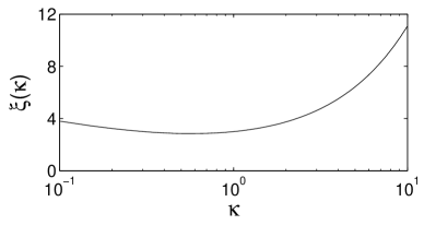
Figure 1: The function $\xi(\kappa)$.

Using $a_{\rho}\equiv\sqrt{\hbar/M\omega_{\rho}}$ ($\hbar\omega_{\rho}$) as unit for length (energy), the dimensionless form of energy per atom becomes

$${\cal E}(q_{\rho},q_{z}) = \frac{1}{4}\left(\frac{2}{q_{\rho}^{2}}+\frac{1}{q_{z}^{2}}\right)+\frac{1}{4}(2q_{\rho}^{2}+\lambda^{2}q_{z}^{2})$$ (10)

$$+\frac{{\cal P}_{\rm ss}}{2q_{\rho}^{2}q_{z}}+\frac{{\cal P}_{\rm sd}}{2q_{\rho}^{2}q_{z}}\chi(\kappa),$$

where $q_{\rho,z}=w_{\rho,z}/a_{\rho}$. The contact and dipolar interaction parameters are ${\cal P}_{\rm ss}=\sqrt{2/\pi}\,Na_{\rm ss}/a_{\rho}$ and ${\cal P}_{\rm sd}=-\sqrt{5/(2\pi)}\,Na_{\rm sd}/a_{\rho}$. The condensate widths $(q_{\rho 0},q_{z0})$ are obtained through a minimization according to

$$\left.\frac{\partial{\cal E}}{\partial q_{\rho}}\right|_{q_{\rho}=q_{\rho 0},q_{z}=q_{z0}}=\left.\frac{\partial{\cal E}}{\partial q_{z}}\right|_{q_{\rho}=q_{\rho 0},q_{z}=q_{z0}}=0,$$

which yield

$$q_{\rho 0} = \frac{1}{q_{\rho 0}^{3}}+\frac{{\cal P}_{\rm ss}}{q_{\rho 0}^{3}q_{z0}}+\frac{{\cal P}_{\rm sd}}{q_{\rho 0}^{3}q_{z0}}f(\kappa_{0}),$$ (11)

$$\lambda^{2}q_{z0} = \frac{1}{q_{z0}^{3}}+\frac{{\cal P}_{\rm ss}}{q_{\rho 0}^{2}q_{z0}^{2}}+\frac{{\cal P}_{\rm sd}}{q_{\rho 0}^{2}q_{z0}^{2}}g(\kappa_{0}),$$ (12)

where $\kappa_{0}=q_{\rho 0}/q_{z0}$ and

$$f(\kappa) = \frac{1}{2(\kappa^{2}-1)^{2}}\left[4\kappa^{4}+7\kappa^{2}-2-9\kappa^{4}H(\kappa)\right]$$

$$-\frac{3}{5}\left[1-(\kappa^{2}-2)H(\kappa)\right],$$

$$g(\kappa) = \frac{1}{(\kappa^{2}-1)^{2}}\left[2\kappa^{4}-10\kappa^{2}-1+9\kappa^{2}H(\kappa)\right]$$

$$+\frac{6}{5}\left[1+(2\kappa^{2}-1)H(\kappa)\right].$$

A solution $(q_{\rho 0},q_{z0})$ is stable if

$$\left[\frac{\partial^{2}{\cal E}}{\partial q_{\rho}^{2}}\frac{\partial^{2}{\cal E}}{\partial q_{z}^{2}}-\left(\frac{\partial^{2}{\cal E}}{\partial q_{\rho}\partial q_{z}}\right)^{2}\right]_{q_{\rho}=q_{\rho 0},q_{z}=q_{z0}}>0.$$ (13)

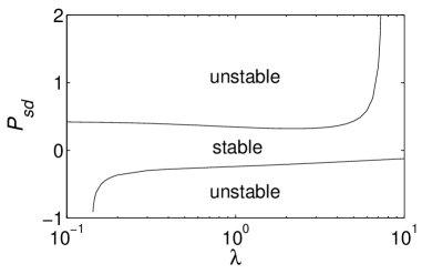
Figure 2: The stability diagram of a dipolar condensate when ${\cal P}_{\rm ss}=0$.

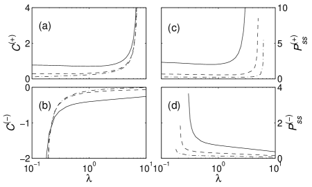
Figure 3: The stability diagram for a dipolar condensate with $a_{\rm ss}>0$. (a) and (b): the $\lambda$ dependence of ${\cal C}^{(\pm)}$ for ${\cal P}_{\rm ss}=1$ (solid line), $10$ (dashed line), and $\infty$ (dash-dotted line); (c) and (d): the $\lambda$ dependence of ${\cal P}_{\rm ss}^{(+)}$ (c) and ${\cal P}_{\rm ss}^{(-)}$ (d) for ${\cal C}=\pm 0.5$ (solid line), $\pm 1$ (dashed line), and $\pm 2$ (dash-dotted line).

We note $\lambda$ is tunable as mentioned before, one can also vary $a_{\rm ss}$ with a Feshbach resonance stoof ; cornish . Close to dipolar induced shape resonances, $a_{\rm sd}$ can be similarly tuned to large or small and positive or negative mircea . The positive valued $a_{\rm sd}$ can be easily understood by considering the interaction between two polarized dipoles. If they were placed in a plane perpendicular to their polarization ($\uparrow\uparrow$), they attract each other; while they repel each other when placed along the direction of their polarization ($\rightarrow\rightarrow$), (note the difference with respect to the bare dipolar interaction yi1 ). Based on these considerations, we proceed to study the properties of a dipolar condensate by varying ${\cal P}_{\rm ss}$, ${\cal P}_{\rm sd}$, and $\lambda$.

Figure 2 shows the stability diagram of a dipolar condensate when $a_{\rm ss}=0$. For $a_{\rm sd}<0$, the condensate is stable if ${\cal P}_{\rm sd}<{\cal P}_{\rm sd}^{(+)}$ and there exists an ‘always stable’ region if $\lambda>\lambda_{+}\simeq 7.56$, which is greater than the previous estimate yi2 ; santos . Interestingly, for $a_{\rm sd}>0$, the condensate is stable if ${\cal P}_{\rm sd}>{\cal P}_{\rm sd}^{(-)}$ and it is always stable for $\lambda<\lambda_{-}\simeq 0.142$.

When $a_{\rm ss}>0$, it is convenient to define ${\cal C}\equiv{\cal P}_{\rm sd}/{\cal P}_{\rm ss}$ which measures the relative strength of the dipolar interaction. $\cal C$ can be changed by tuning $a_{\rm sd}$. As shown in Fig. 3 (a) and (b), for a given $a_{\rm ss}>0$, the condensate is stable if ${\cal C}^{(-)}<{\cal C}<{\cal C}^{(+)}$. Similar to the previous result yi2 , the critical value of $\lambda$ for the ‘always stable’ region is approximately $\cal C$-independent and equal to $\lambda_{\pm}$ for $a_{\rm ss}=0$. For a fixed $\cal C$, the condensate stability can be modified by tuning ${\cal P}_{\rm ss}$. From Fig. 3 (c) and (d), we see that only when ${\cal P}_{\rm ss}<{\cal P}_{\rm ss}^{(+)}$ for ${\cal C}>0$ and ${\cal P}_{\rm ss}<{\cal P}_{\rm ss}^{(-)}$ for ${\cal C}<0$ is the condensate stable. Varying ${\cal P}_{\rm ss}$ for a constant $\cal C$ can be achieved by changing $N$.

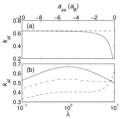
Figure 4: (a) The dependence of $k_{\rm st}$ on $a_{\rm ss}$ for $\lambda=6.8/17.35$. The dashed line is the result without dipolar interaction. (b) The dependence of $k_{\rm st}$ on $\lambda$ for $a_{\rm ss}=-0.5(a_{B})$ (dashed line), $-1(a_{B})$ (dash-dotted line), and $-4(a_{B})$ (dotted line). The solid line is the result without dipolar interaction.

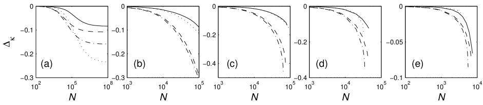
Figure 5: The $N$ dependence of $\Delta_{k}$ for $a_{\rm ss}=5(a_{B})$ (a), $0.5$ (b), $0$ (c), $-0.5$ (d), $-5$ (e), and $\lambda=0.2$ (solid line), $0.6$ (dashed line), $2$ (dash-dotted line), $6$ (dotted line).

When $a_{\rm ss}<0$, the condensate becomes unstable if $N$ exceeds a critical value $N_{\rm cr}$ even without dipolar interaction. This instability is typically measured by the stability coefficient $k_{\rm st}\equiv N_{\rm cr}|a_{\rm sc}|/a_{\rm ho}$ ane ; garmmal with $a_{\rm ho}=\sqrt{\hbar/m\bar{\omega}}$ and $\bar{\omega}=(\omega_{x}\omega_{y}\omega_{z})^{1/3}$. To study the dipolar induced modification of $k_{\rm st}$, we consider the experiment donley ; cornish of ⁸⁵Rb atoms in state $|F=2,M_{F}=2\rangle$ with a magnetic dipole moment of $\mu=2\mu_{B}/3$. We take $a_{\rm sd}$ as obtained for the multi-channel scattering calculation mircea . For $\omega_{\rho}=(2\pi)17.35$ (Hz), we then have ${\cal P}_{\rm sd}\approx 5.0\times 10^{-6}N$. Figure 4 (a) shows the $a_{\rm ss}$ dependence of $k_{\rm st}$ for $\lambda=6.8/17.35$. As before dipolar interaction destabilizes a condensate for this configuration; However, the enhanced effect due to the more rigorous pseudo-potential Eq. (6) is more profound: even for $a_{\rm ss}<-3(a_{B})$, the effect of dipolar interaction is still visible. In Fig. 4 (b), we plot the $\lambda$ dependence of $k_{\rm st}$. Since ${\cal P}_{\rm sd}>0$, dipolar interaction destabilizes the condensate at small values of $\lambda$; when $\lambda$ is large, dipolar interaction can also stabilize an otherwise attractive condensate.

Finally, we briefly consider the condensate aspect ratio $\kappa_{0}$. We define its relative change yi3

$$\Delta_{\kappa}\equiv\frac{\kappa_{0}({\cal P}_{\rm sd}\neq 0)-\kappa_{0}({\cal P}_{\rm sd}=0)}{\kappa_{0}({\cal P}_{\rm sd}=0)}$$ (14)

as a measure of whether it is possible to detect the dipolar interaction from imaging condensate shape within current experiments. Figure 5 shows its $N$-dependence for various $a_{\rm ss}$ and $\lambda$. For certain $\lambda$, $\Delta_{\kappa}$ can be as high as 20% even with $N=2\times 10^{5}$, if $|a_{\rm ss}|$ is tuned small.

In conclusion, we have calibrated the properties of a dipolar condensate using the more rigorous anisotropic pseudo-potential andrei1 , based on a variational calculation. Significant enhancement were found to all dipolar effects predicted previously. In the limit of weak s-wave interactions, when $P_{\rm ss}\leq 1$ due to a small $a_{\rm ss}$ and/or a small $N$, our results are clearly valid based on previous studies with the same variational technique yi2 ; yi3 ; yi4 ; var ; var1 , where extensively comparisons were preformed to justify the trial function Eq. (7) var ; var1 , including the presence of a weak dipolar interaction yi2 ; yi3 ; yi4 . We note this is also the interesting limit where experimental detection of coherent dipolar interactions will likely occur. The variation approach gives reliable stationary condensate properties, although not the density profile itself, even when the interaction energy is large var1 . The results from $P_{\rm ss}>1$, although consistent, needs further improvements with more accurate numerical calculations (over the present variational method).

We acknowledge insightful discussions and communications with Dr. Derevianko. This work is supported by NSF and NSFC.

References

• (1) Current address: Department of Physics and Astronomy, and Rice Quantum Institute, Rice University, Houston, TX 77251-1892, USA.
• (2) M. Marinescu and L. You, Phys. Rev. Lett. 81, 4596 (1998); B. Deb and L. You, Phys. Rev. A 64, 022717 (2001).
• (3) S. Yi and L. You, Phys. Rev. A 61, 041604(R) (2000).
• (4) K. Goral et al., Phys. Rev. A 61, 051601(R) (2000); J.-P. Martikainen et al., Phys. Rev. A 64, 037601 (2001).
• (5) L. Santos et al., Phys. Rev. Lett. 85, 1791 (2000); ibid 88, 139904(E) (2002).
• (6) S. Yi and L. You, Phys. Rev. A 63, 053607 (2001).
• (7) S. Yi and L. You, Phys. Rev. A 66, 013607 (2002).
• (8) K. Goral and L. Santos, Phys. Rev. A 66, 023613 (2002).
• (9) D. H. J. O’Dell et al., Phys. Rev. Lett. 90, 110402 (2003).
• (10) L. Santos et al., Phys. Rev. Lett. 90, 250403 (2003).
• (11) S. Yi and L. You, Phys. Rev. A 67, 045601 (2003).
• (12) S. Giovanazzi et al., J Opt. B 5, S208 (2003).
• (13) K. Goral et al., Phys. Rev. Lett. 88, 170406 (2002).
• (14) C. Eberlein et al., (cond-mat/0311100).
• (15) K. Huang and C. N. Yang, Phys. Rev. 105, 767 (1957).
• (16) A. Derevianko, Phys. Rev. A 67, 033607 (2003).
• (17) A. Derevianko, (private communication); K. Huang, Statistical Mechanics, 2nd Ed. (Wiley, New York, 1987).
• (18) G. Baym and C. J. Pethick, Phys.Β Rev.Β Lett.Β 76, 6 (1996).
• (19) Victor M. Perez-Garcia et al., Phys. Rev. Lett. 77, 5320 (1996); Phys. Rev. A 56, 1424 (1997).
• (20) M. Olshanii, Phys. Rev. Lett. 81, 938 (1998).
• (21) E. Tiesinga et al., Phys. Rev. A 47, 4114 (1993).
• (22) S. L. Cornish et al., Phys. Rev. Lett. 85, 1795 (2000).
• (23) P. A. Ruprecht et al., Phys. Rev. A 51, 4704 (1995); C. A. Sackett et al., Phys. Rev. Lett. 80, 2031 (1998).
• (24) A. Gammal et al., Phys. Rev. A 64, 055602 (2001); V. S. Filho et al., ibid 66, 043605 (2002).
• (25) E. A. Donley et al., Nature 412, 295 (2001).