Antibunched photons emitted by a quantum point contact out of equilibrium

Abstract

Motivated by the experimental search for “GHz nonclassical light”, we identify the conditions under which current fluctuations in a narrow constriction generate sub-Poissonian radiation. Antibunched electrons generically produce bunched photons, because the same photon mode can be populated by electrons decaying independently from a range of initial energies. Photon antibunching becomes possible at frequencies close to the applied voltage $V\times e/\hbar$, when the initial energy range of a decaying electron is restricted. The condition for photon antibunching in a narrow frequency interval below $eV/\hbar$ reads $[\sum_{n}T_{n}(1-T_{n})]^{2}<2\sum_{n}[T_{n}(1-T_{n})]^{2}$, with $T_{n}$ an eigenvalue of the transmission matrix. This condition is satisfied in a quantum point contact, where only a single $T_{n}$ differs from 0 or 1. The photon statistics is then a superposition of binomial distributions.

In a recent experiment Gab04 , Gabelli et al. have measured the deviation from Poisson statistics of photons emitted by a resistor in equilibrium at mK temperatures. By cross-correlating the power fluctuations they detected photon bunching, meaning that the variance ${\rm Var}\,n=\langle n^{2}\rangle-\langle n\rangle^{2}$ in the number of detected photons exceeds the mean photon count $\langle n\rangle$. Their experiment is a variation on the quantum optics experiment of Hanbury Brown and Twiss Han56 , but now at GHz frequencies.

In the discussion of the implications of their novel experimental technique, Gabelli et al. noticed that a general theory Bee01 for the radiation produced by a conductor out of equilibrium implies that the deviation from Poisson statistics can go either way: Super-Poissonian fluctuations (${\rm Var}\,n>\langle n\rangle$, signaling bunching) are the rule in conductors with a large number of scattering channels, while sub-Poissonian fluctuations (${\rm Var}\,n<\langle n\rangle$, signaling antibunching) become possible in few-channel conductors. They concluded that a quantum point contact could therefore produce GHz nonclassical light Man95 .

It is the purpose of this work to identify the conditions under which electronic shot noise in a quantum point contact can generate antibunched photons. The physical picture that emerges differs in one essential aspect from electron-hole recombination in a quantum dot or quantum well, which is a familiar source of sub-Poissonian radiation Kim99 ; Mic00 ; Yua02 . In those systems the radiation is produced by transitions between a few discrete levels. In a quantum point contact the transitions cover a continuous range of energies in the Fermi sea. As we will see, this continuous spectrum generically prevents antibunching, except at frequencies close to the applied voltage.

Before presenting a quantitative analysis, we first discuss the mechanism in physical terms. As depicted in Fig. 1, electrons are injected through a constriction in an energy range $eV$ above the Fermi energy $E_{F}$, leaving behind holes at the same energy. The statistics of the charge $Q$ transferred in a time $\tau\gg\hbar/eV$ is binomial Lev93 , with ${\rm Var}\,Q/e<\langle Q/e\rangle$. This electron antibunching is a result of the Pauli principle. Each scattering channel $n=1,2,\ldots N$ in the constriction and each energy interval $\delta E=\hbar/\tau$ contributes independently to the charge statistics. The photons excited by the electrons would inherit the antibunching if there would be a one-to-one correspondence between the transfer of an electron and the population of a photon mode. Generically, this is not what happens: A photon of frequency $\omega$ can be excited by each scattering channel and by a range $eV-\hbar\omega$ of initial energies. The resulting statistics of photocounts is negative binomial Bee01 , with ${\rm Var}\,n>\langle n\rangle$. This is the same photon bunching as in black-body radiation note0 .

In order to convert antibunched electrons into antibunched photons, it is sufficient to ensure a one-to-one correspondence between electron modes and photon modes. This can be realized by concentrating the current fluctuations in a single scattering channel and by restricting the energy range $eV-\hbar\omega$. Indeed, in a single-channel conductor and in a narrow frequency range $\omega\lesssim eV/\hbar$ we obtain sub-Poissonian photon statistics regardless of the value of the transmission probability. In the more general multi-channel case, photon antibunching is found if $[\sum_{n}T_{n}(1-T_{n})]^{2}<2\sum_{n}[T_{n}(1-T_{n})]^{2}$ (with $T_{n}$ an eigenvalue of the transmission matrix product $tt^{\dagger}$).

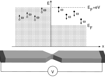
Figure 1: Schematic diagram of a constriction in a conductor (bottom) and the energy range of electronic states (top), showing excitations of electrons (black dots) and holes (white dots) in the Fermi sea. A voltage $V$ drops over the constriction. Electrons (holes) in an energy range $eV-\hbar\omega$ can populate a photon mode of frequency $\omega$, by decaying to an empty (filled) state closer to the Fermi level.

Starting point of our quantitative analysis is the general relationship of Ref. Bee01 between the photocount distribution $P(n)$ and the expectation value of an ordered exponential of the electrical current operator:

$$P(n)=\frac{1}{n!}\lim_{\xi\rightarrow-1}\frac{d^{n}}{d\xi^{n}}F(\xi),$$ (1)

$$F(\xi)=\left\langle{\cal O}\exp\left[\xi\int_{0}^{\infty}d\omega\,\gamma(\omega)I^{\dagger}(\omega)I(\omega)\right]\right\rangle.$$ (2)

We summarize the notation. The function $F(\xi)=\sum_{k=0}^{\infty}(\xi^{k}/k!)\langle n^{k}\rangle_{\rm f}$ is the generating function of the factorial moments $\langle n^{k}\rangle_{\rm f}\equiv\langle n(n-1)(n-2)\cdots(n-k+1)\rangle$. The current operator $I=I_{\rm out}-I_{\rm in}$ is the difference of the outgoing current $I_{\rm out}$ (away from the constriction) and the incoming current $I_{\rm in}$ (toward the constriction). The symbol $\cal O$ indicates ordering of the current operators from left to right in the order $I_{\rm in}^{\dagger},I_{\rm out}^{\dagger},I_{\rm out}^{\vphantom{\dagger}},I_{\rm in}^{\vphantom{\dagger}}$. The real frequency-dependent response function $\gamma(\omega)$ is proportional to the coupling strength of conductor and photodetector and proportional to the detector efficiency. Positive (negative) $\omega$ corresponds to absorption (emission) of a photon by the detector. We consider photodetection by absorption, hence $\gamma(\omega)\equiv 0$ for $\omega\leq 0$. Integrals over frequency should be interpreted as sums over discrete modes $\omega_{p}=p\times 2\pi/\tau$, $p=1,2,3,\ldots$. The detection time $\tau$ is sent to infinity at the end of the calculation. We denote $\gamma_{p}=\gamma(\omega_{p})\times 2\pi/\tau$, so that $\int d\omega\,\gamma(\omega)\rightarrow\sum_{p}\gamma_{p}$. For ease of notation we set $\hbar=1$, $e=1$.

The exponent in Eq. (2) is quadratic in the current operators, which complicates the calculation of the expectation value. We remove this complication by introducing a Gaussian field $z(\omega)$ and performing a Hubbard-Stratonovich transformation,

$$F(\xi) = \left\langle{\cal O}\exp\left[\sqrt{\xi}\int_{0}^{\infty}d\omega\,\gamma(\omega)[z(\omega)I^{\dagger}(\omega)\right.\right.$$ (3)

$$\mbox{}+\left.\left.\vphantom{\int_{0}^{\infty}}z^{\ast}(\omega)I(\omega)]\right]\right\rangle.$$

The brackets $\langle\cdots\rangle$ now indicate both a quantum mechanical expectation value of the current operators and a classical average over independent complex Gaussian variables $z_{p}=z(\omega_{p})$ with zero mean and variance $\langle|z_{p}|^{2}\rangle=1/\gamma_{p}$.

We assume zero temperature, so that the incoming current is noiseless. We may then replace $I$ by $I_{\rm out}$ and restrict ourselves to energies $\varepsilon$ in the range $(0,V)$ above $E_{F}$. Let $b_{n}^{\dagger}(\varepsilon)$ be the operator that creates an outgoing electron in scattering channel $n$ at energy $\varepsilon$. The outgoing current is given in terms of the electron operators by

$$I_{\rm out}(\omega)=\int_{0}^{V}d\varepsilon\,\sum_{n}b^{\dagger}_{n}(\varepsilon)b^{\vphantom{\dagger}}_{n}(\varepsilon+\omega).$$ (4)

Energy $\varepsilon_{p}=p\times 2\pi/\tau$ is discretized in the same way as frequency. The energy and channel indices $p,n$ are collected in a vector $b$ with elements $b_{pn}=(2\pi/\tau)^{1/2}b_{n}(\epsilon_{p})$. Substitution of Eq. (4) into Eq. (3) gives

$$F(\xi)=\left\langle e^{b^{\dagger}Zb}e^{b^{\dagger}Z^{\dagger}b}\right\rangle.$$ (5)

The exponents contain the product of the vectors $b,b^{\dagger}$ and a matrix $Z$ with elements $Z_{pn,p^{\prime}n^{\prime}}=\xi^{1/2}\delta_{nn^{\prime}}z_{p-p^{\prime}}\gamma_{p-p^{\prime}}$. Notice that $Z$ is diagonal in the channel indices $n,n^{\prime}$ and lower-triangular in the energy indices $p,p^{\prime}$.

Because of the ordering ${\cal O}$ of the current operators, the single exponential of Eq. (3) factorizes into the two noncommuting exponentials of Eq. (5). In order to evaluate the expectation value efficiently, we would like to bring this back to a single exponential — but now with normal ordering ${\cal N}$ of the fermion creation and annihilation operators. (Normal ordering means $b^{\dagger}$ to the left of $b$, with a minus sign for each permutation.) This is accomplished by means of the operator identity note1

$$\prod_{i}e^{b^{\dagger}A_{i}b}={\cal N}\exp\left[b^{\dagger}\left(\prod_{i}e^{A_{i}}-1\right)b\right],$$ (6)

valid for any set of matrices $A_{i}$. The quantum mechanical expectation value of a normally ordered exponential is a determinant Cah99 ,

$$\langle{\cal N}e^{b^{\dagger}Ab}\rangle={\rm Det}\,(1+AB),\;\;B_{ij}=\langle b_{j}^{\dagger}b_{i}^{\vphantom{\dagger}}\rangle.$$ (7)

In our case $A=e^{Z}e^{Z^{\dagger}}-1$ and $B=tt^{\dagger}$, with $t$ the $N\times N$ transmission matrix of the constriction.

In the experimentally relevant case Agu00 ; Gab04 the response function $\gamma(\omega)$ is sharply peaked at a frequency $\Omega\lesssim V$, with a width $\Delta\ll\Omega$. We assume that the energy dependence of the transmission matrix may be disregarded on the scale of $\Delta$, so that we may choose an $\varepsilon$-independent basis in which $tt^{\dagger}$ is diagonal. The diagonal elements are the transmission eigenvalues $T_{1},T_{2},\ldots T_{N}\in(0,1)$. Combining Eqs. (5–7) we arrive at

$$F(\xi) = \left\langle\prod_{n=1}^{N}{\rm Det}\,\left[1+T_{n}\bigl{(}e^{Z}e^{Z^{\dagger}}-1\bigr{)}\right]\right\rangle$$ (8)

$$= \left\langle\prod_{n=1}^{N}{\rm Det}\,\left[(1-T_{n})e^{-Z^{\dagger}}+T_{n}e^{Z}\right]\right\rangle.$$

(In the second equality we used that ${\rm Det}\,e^{Z^{\dagger}}=1$, since $Z$ is a lower-triangular matrix.) The remaining average is over the Gaussian variables $z_{p}$ contained in the matrix $Z$.

Since the interesting new physics occurs when $\Omega$ is close to $V$, we simplify the analysis by assuming that $\gamma(\omega)\equiv 0$ for $\omega<V/2$. For such a response function one has $Z^{2}=0$. (This amounts to the statement that no electron with excitation energy $\varepsilon<V$ can produce more than a single photon of frequency $\omega>V/2$.) We may therefore replace $e^{Z}\rightarrow 1+Z$ and $e^{-Z^{\dagger}}\rightarrow 1-Z^{\dagger}$ in Eq. (8). We then apply the matrix identity

$${\rm Det}\,(1+A+B)={\rm Det}\,(1-AB),\;\;{\rm if}\;\;A^{2}=0=B^{2},$$ (9)

and obtain

$$F(\xi) = \prod_{p}\frac{\gamma_{p}}{\pi}\int d^{2}z_{p}\,e^{-\gamma_{p}|z_{p}|^{2}}$$ (10)

$$\mbox{}\times\prod_{n=1}^{N}{\rm Det}\,[1+T_{n}(1-T_{n})\xi X].$$

We have defined $\xi X\equiv ZZ^{\dagger}$ and written out the Gaussian average. The Hermitian matrix $X$ has elements

$$X_{pp^{\prime}}=\sum_{q}z^{\vphantom{\ast}}_{p-q}z^{\ast}_{p^{\prime}-q}\gamma_{p-q}\gamma_{p^{\prime}-q}.$$ (11)

The integers $p,p^{\prime},q$ range from $1$ to $V\tau/2\pi$.

The Gaussian average is easy if the dimensionless shot noise power $S=\sum_{n}T_{n}(1-T_{n})$ is $\gg 1$. We may then do the integrals of Eq. (10) in saddle-point approximation, with the result note2

$$\ln F(\xi)=-\frac{\tau}{2\pi}\int_{0}^{V}d\omega\,\ln\left[1-\xi S\gamma(\omega)(V-\omega)\right].$$ (12)

The logarithm $\ln F(\xi)$ is the generating function of the factorial cumulants $\langle\!\langle n^{k}\rangle\!\rangle_{\rm f}$ note3 . By expanding Eq. (12) in powers of $\xi$ we find

$$\langle\!\langle n^{k}\rangle\!\rangle_{\rm f}=(k-1)!\frac{\tau}{2\pi}\int_{0}^{V}d\omega\,[S\gamma(\omega)(V-\omega)]^{k}.$$ (13)

Eqs. (12) and (13) represent the multi-mode superposition of independent negative-binomial distributions note0 . All factorial cumulants are positive, in particular the second, so ${\rm Var}\,n>\langle n\rangle$. This is super-Poissonian radiation.

When $S$ is not $\gg 1$, e.g. when only a single channel contributes to the shot noise, the result (12-13) remains valid if $V-\Omega\gg\Delta$. This was the conclusion of Ref. Bee01 , that narrow-band detection leads generically to a negative-binomial distribution. However, the saddle-point approximation breaks down when the detection frequency $\Omega$ approaches the applied voltage $V$. For $V-\Omega\lesssim\Delta$ one has to calculate the integrals in Eq. (10) exactly.

We have evaluated the generating function (10) for a response function of the block form

$$\gamma(\omega)=\left\{\begin{array}[]{l}\gamma_{0}\;\;{\rm if}\;\;V-\Delta<\omega<V,\\ 0\;\;{\rm if}\;\;\omega<V-\Delta,\end{array}\right.$$ (14)

with $\Delta<V/2$. The frequency dependence for $\omega>V$ is irrelevant. In the case $N=1$ of a single channel, with transmission probability $T_{1}\equiv T$, we find note4

$$\ln F(\xi) = \frac{\tau}{2\pi}\int_{V-\Delta}^{V}d\omega\,\ln\left[1+\xi\gamma_{0}T(1-T)(V-\omega)\right]$$ (15)

$$= \frac{\tau\Delta}{2\pi}\frac{(1+x)\ln(1+x)-x}{x},$$

with $x\equiv\xi\gamma_{0}T(1-T)\Delta$. This is a superposition of binomial distributions. The factorial cumulants are

$$\langle\!\langle n^{k}\rangle\!\rangle_{\rm f}=(-1)^{k+1}\frac{(k-1)!}{k+1}\frac{\tau\Delta}{2\pi}[T(1-T)\gamma_{0}\Delta]^{k}.$$ (16)

The second factorial cumulant is negative, so ${\rm Var}\,n<\langle n\rangle$. This is sub-Poissonian radiation.

We have not found such a simple closed-form expression in the more general multi-channel case, but it is straightforward to evaluate the low-order factorial cumulants from Eq. (10). We find

$$\langle n\rangle=\frac{\tau\Delta}{2\pi}\gamma_{0}\Delta\frac{1}{2}S_{1},$$ (17)

$$\langle\!\langle n^{2}\rangle\!\rangle_{\rm f}=\frac{\tau\Delta}{2\pi}(\gamma_{0}\Delta)^{2}\frac{1}{3}(S_{1}^{2}-2S_{2}),$$ (18)

$$\langle\!\langle n^{3}\rangle\!\rangle_{\rm f}=\frac{\tau\Delta}{2\pi}(\gamma_{0}\Delta)^{3}\frac{1}{6}\left(3S_{1}^{3}-15S_{1}S_{2}+15S_{3}\right),$$ (19)

with $S_{p}=\sum_{n}[T_{n}(1-T_{n})]^{p}$. Antibunching therefore requires $S_{1}^{2}<2S_{2}$.

The condition on antibunching can be generalized to arbitrary frequency dependence of the response function $\gamma(\omega)$ in the range $V-\Delta<\omega<V$ of detected frequencies. For $\Delta<V/2$ we find

$${\rm Var}\,n-\langle n\rangle=\frac{\tau}{2\pi}\int_{V-\Delta}^{V}d\omega^{\prime}\,\gamma(\omega^{\prime})\int_{\omega^{\prime}}^{V}d\omega\,(V-\omega)$$

$$\;\;\;\mbox{}\times\left(2S_{1}^{2}-4S_{2}-(V-\omega)S_{1}^{2}\frac{d}{d\omega}\right)\gamma(\omega).$$ (20)

We see that the antibunching condition $S_{1}^{2}<2S_{2}$ derived for the special case of the block function (14) is more generally a sufficient condition for antibunching to occur, provided that $d\gamma/d\omega\geq 0$ in the detection range. It does not matter if the response function drops off at $\omega>V$, provided that it increases monotonically in the range $(V-\Delta,V)$. A steeply increasing response function in this range is more favorable, but not by much. For example, the power law $\gamma(\omega)\propto(\omega-V+\Delta)^{p}$ gives the antibunching condition $S_{1}^{2}<2S_{2}\times[1+p/(1+p)]$, which is only weakly dependent on the power $p$.

In conclusion, we have presented both a qualitative physical picture and a quantitative analysis for the conversion of electron to photon antibunching. A simple criterion, Eq. (18), is obtained for sub-Poissonian photon statistics, in terms of the transmission eigenvalues $T_{n}$ of the conductor. Since an $N$-channel quantum point contact has only a single $T_{N}$ different from 0 or 1, it should generate antibunched photons in a frequency band $(V-\Delta,V)$ — regardless of the value of $T_{N}$. The statistics of these photons is the superposition (15) of binomial distributions, inherited from the electronic binomial distribution. There are no stringent conditions on the band width $\Delta$, as long as it is $<V/2$ (in order to prevent multi-photon excitations by a single electron note5 ). This should make it feasible to use the cross-correlation technique of Ref. Gab04 to detect the emission of nonclassical microwaves by a quantum point contact.

We have benefitted from correspondence with D. C. Glattli. This work was supported by the Dutch Science Foundation NWO/FOM.

References

- (1) J. Gabelli, L.-H. Reydellet, G. Fève, J.-M. Berroir, B. Plaçais, P. Roche, and D. C. Glattli, cond-mat/0403584.
- (2) R. Hanbury Brown and R. Q. Twiss, Nature 177, 27 (1956).
- (3) C. W. J Beenakker and H. Schomerus, Phys. Rev. Lett. 86, 700 (2001).
- (4) Sub-Poissonian radiation is called “nonclassical”, because its photocount statistics can not be interpreted in classical terms as a superposition of Poisson processes. See L. Mandel and E. Wolf, Optical Coherence and Quantum Optics (Cambridge University, Cambridge, 1995).
- (5) J. Kim, O. Benson, H. Kan, and Y. Yamamoto, Nature 397, 500 (1999); C. Santori, M. Pelton, G. Solomon, Y. Dale, and Y. Yamamoto, Phys. Rev. Lett. 86, 1502 (2001).
- (6) P. Michler, A. Imamoǧlu, M. D. Mason, P. J. Carson, G. F. Strouse, and S. K. Buratto, Nature 406, 968 (2000); P. Michler, A. Kiraz, C. Becher, W. V. Schoenfeld, P. M. Petroff, L. Zhang, E. Hu, and A. Imamoǧlu, Science 290, 2282 (2000).
- (7) Z. L. Yuan, B. E. Kardynal, R. M. Stevenson, A. J. Shields, C. J. Lobo, K. Cooper, N. S. Beattie, D. A. Ritchie, and M. Pepper, Science 295, 102 (2002).
- (8) L. S. Levitov and G. B. Lesovik, JETP Lett. 58, 230 (1993).
- (9) The negative-binomial distribution counts the number of partitions of bosons among states in a frequency interval . The binomial distribution counts the number of partitions of fermions among states.
- (10) Eq. (6) is the multi-matrix generalization of the well known identity .
- (11) K. E. Cahill and R. J. Glauber, Phys. Rev. A 59, 1538 (1999).
- (12) R. Aguado and L. P. Kouwenhoven, Phys. Rev. Lett. 84, 1986 (2000).
- (13) The saddle point is at , so to integrate out the Gaussian fluctuations around the saddle point we may linearize the determinant in Eq. (10): . The result is Eq. (12).
- (14) Factorial cumulants are constructed from factorial moments in the usual way. The first two are: , .
- (15) Using computer algebra, we find that , for each matrix dimensionality that we could check. We are confident that this closed form holds for all , but we have not yet found an analytical proof. Eq. (15) follows in the limit upon conversion of the summation into an integration.
- (16) Multi-photon excitations do not contribute to if for all [cf. Ref. Bee01 , Eq. (19)]. For a quantum point contact, one finds that antibunching persists when provided that .