Shadow on the wall cast by an Abrikosov vortex

Abstract

At the surface of a $d$-wave superconductor, a zero-energy peak in the quasiparticle spectrum can be observed. This peak appears due to Andreev bound states and is maximal if the nodal direction of the $d$-wave pairing potential is perpendicular to the boundary. We examine the effect of a single Abrikosov vortex in front of a reflecting boundary on the zero-energy density of states. We can clearly see a splitting of the low-energy peak and therefore a suppression of the zero-energy density of states in a shadow-like region extending from the vortex to the boundary. This effect is stable for different models of the single Abrikosov vortex, for different mean free paths and also for different distances between the vortex center and the boundary. This observation promises to have also a substantial influence on the differential conductance and the tunneling characteristics for low excitation energies.

Today, there is common agreement that most high-$T_{c}$ superconductors exhibit $d$-wave symmetry. An important characteristic of $d$-wave superconductors is the possible existence of Andreev bound states at its surface Hu ; Tanaka ; Buchholtz . This increase of the local zero-energy quasiparticle density of states at the surface can clearly be observed in the differential tunneling conductance as a pronounced zero-bias conductance peak Iguchi ; Lesueur ; Covington . For specular boundaries, this peak reaches maximum height, if the surface is perpendicular to the nodal direction of the $d$-wave. The effect shrinks, if the orientation is changed Tanaka ; Iguchi . For an angle of 45 degrees between the nodal direction and the surface the bound states have vanished completely. However, it has been pointed out, that for rough surfaces a similar shape of the zero-bias conductance peak is obtained which is independent of the boundary orientation Fogelstroem . If a magnetic field is applied, the spectral weight of the zero-bias peak decreases and a splitting of the peak is observed CovingtonAprili ; Aprili ; Dagan .

In this Letter, we study a single Abrikosov vortex in front of a specular surface, and we investigate the effect of the vortex on the local quasiparticle density of states along the boundary. All interesting phenomena of this problem are described within the quasiclassical theory, which is valid if the coherence length is much larger than the Fermi wavelength. To calculate the local density of states in the vicinity of the boundary it is necessary to find numerically stable solutions of the Eilenberger equations Eilenberger ; Larkin that fulfill the appropriate boundary conditions at the specular surface. For this purpose we use the Riccati parametrization of the quasiclassical propagator SchopohlMaki . Along a trajectory of the kind ${\bm{r}}(x)={\bm{r}}_{0}+x\;{\bm{v}}_{F}$ the Eilenberger equations of superconductivity reduce to a set of two decoupled differential equations of the Riccati type for the functions $a(x)$ and $b(x)$

$$\hbar v_{F}\partial_{x}a(x)+\left[2\tilde{\epsilon}_{n}+\Delta^{\dagger}a(x)\right]a(x)-\Delta = 0$$

$$\hbar v_{F}\partial_{x}b(x)-\left[2\tilde{\epsilon}_{n}+\Delta b(x)\right]b(x)+\Delta^{\dagger} = 0$$ (1)

where $i\tilde{\epsilon}_{n}=i\epsilon_{n}+{\bm{v}}_{F}\cdot\frac{e}{c}{\bm{A}}$ are shifted Matsubara frequencies. For the simple case of a cylindrical Fermi surface the Fermi velocity can be written as

$${\bm{v}}_{F}=v_{F}({\bm{e}}_{1}\cos\theta+{\bm{e}}_{2}\sin\theta)$$ (2)

The $\theta$- and ${\bm{r}}$-dependence of the pairing potential $\Delta$ can be factorized in the form

$$\Delta({\bm{r}},\theta)=\Delta_{0}\chi(\theta)\Psi({\bm{r}})$$ (3)

For a $d_{x^{2}-y^{2}}$-wave superconductor the symmetry function takes the form $\chi(\theta)=\cos(2\theta)$ and for the $s$-wave symmetry it becomes constant $\chi(\theta)=1$. For $\epsilon_{n}>0$ the Riccati equations have to be solved using the bulk values as initial values at $x=\pm\infty$

$$a(-\infty)=\frac{\Delta(-\infty)}{\epsilon_{n}+\sqrt{\epsilon_{n}^{2}+|\Delta(-\infty)|^{2}}}$$

$$b(+\infty)=\frac{\Delta^{\dagger}(+\infty)}{\epsilon_{n}+\sqrt{\epsilon_{n}^{2}+|\Delta(+\infty)|^{2}}}$$ (4)

The numerical solution of the Riccati equations can be done with minor effort and leads to rapidly converging results. For the calculation of the local density of states the imaginary part of the quasiclassical propagator has to be integrated over the angle $\theta$ that defines the direction of the Fermi velocity. In terms of $a$ and $b$ we have

$$N({\bm{r}}_{0},E)=\int_{0}^{2\pi}\frac{d\theta}{2\pi}{\rm Re}\;\left[\frac{1-ab}{1+ab}\right]_{i\epsilon_{n}\rightarrow E+i\delta}$$ (5)

where $E$ denotes the quasiparticle energy with respect to the Fermi level and $\delta$ is an effective scattering parameter that corresponds to an inverse mean free path. As it is well known, the localized zero-energy state in a $d_{x^{2}-y^{2}}$-superconductor at a specular 110-boundary arises from the sign change in the pairing potential on a quasiparticle trajectory that is reflected at the surface. The outgoing particles are Andreev reflected at this potential step and interfere with the incident quasiparticles. This interference process leads to stable zero-energy trapped states in the vicinity of the boundary, called Andreev bound states. The same sign change in the order parameter is found on a trajectory that passes near the center of a vortex and therefore leads to similar localized Andreev bound states inside the vortex core. The suppression of the amplitude of the pairing potential around the vortex center gives only a small quantitative correction in the calculation of the trapped state as we already pointed out before DGIS . The influence of the boundary for anisotropic superconductors is included within the quasiclassical theory if the nonlinear boundary conditions for the quasiparticle propagator are applied Zaitsev ; RainerBuchholtz . For the Riccati parametrization a substantial simplification occurs and an explicit solution of the nonlinear boundary conditions can be found Shelankov .

In the following we assume a totally reflecting surface where the transparency ${\mathcal{T}}$ equals zero while the reflectivity ${\mathcal{R}}$ becomes one. In this special case the boundary conditions reduce to

$$a_{\rm out}^{l/r}=a_{\rm in}^{l/r}\hskip 10.00002pt{\rm and}\hskip 10.00002ptb_{\rm in}^{l/r}=b_{\rm out}^{l/r}$$ (6)

In the next step we try to find an appropriate model that describes the pairing potential associated with the single vortex in front of the reflecting boundary. With the condition that there are no currents flowing across the boundary we have to find a phase of the order parameter where the phase gradient vanishes perpendicular to the boundary. In analogy to the classical boundary value problem of electrostatics with a point charge in front of a conducting surface we introduce an image vortex on the opposite site of the reflecting boundary. The pairing potential around a vortex at position ${\bm{r}}_{V}$ can be written as (see also DolgovSchopohl )

$$\Psi({\bm{r}})=f(|{\bm{r}}-{\bm{r}}_{V}|)e^{i\Phi({\bm{r}})}$$ (7)

The function $f(|{\bm{r}}-{\bm{r}}_{V}|)$ characterizes the amplitude of the pairing potential of the single vortex. Since we consider a vortex-antivortex pair, the phase $\Phi({\bm{r}})$ is given as

$$\Phi({\bm{r}})={\rm arg}({\bm{r}}-{\bm{r}}_{V})-{\rm arg}({\bm{r}}-{\bar{\bm{r}}}_{V})$$ (8)

The location of the image vortex behind the boundary is defined by ${\bar{\bm{r}}}_{V}={\bm{r}}_{V}-2\hat{\bm{n}}\langle\hat{\bm{n}},{\bm{r}}_{V}\rangle$. The normal unit vector is given as $\hat{\bm{n}}=1/\sqrt{2}({\bm{e}}_{1}+{\bm{e}}_{2})$ for a 110-boundary.

In the following, the origin $\mathcal{O}$ of our coordinate system is placed at the boundary right between the vortex and the image vortex. The $y$-axis is orientated parallel to the boundary. $x_{V}$ denotes the vortex position on the $x$-axis and also measures the vortex to boundary distance. Furthermore it is useful to introduce the coherence length $\xi=\frac{\hbar v_{F}}{\Delta_{0}}$ as the unit of a general length scale. We performed calculations of the local density of states for both a model pairing potential modulus $f(|{\bm{r}}-{\bm{r}}_{V}|)=\tanh(|{\bm{r}}-{\bm{r}}_{V}|/\xi)$ and a constant modulus $f(|{\bm{r}}-{\bm{r}}_{V}|)=1$. The latter corresponds to a pure phase vortex. The results according to both models show only small quantitative differences. In particular, the main qualitative effect we want to present here, the shadow on the zero-energy density of states, exists independently. Thus, we will restrict our following considerations to the simpler second model.

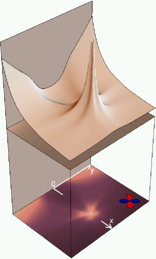
In Fig. 1 we show the zero-energy local density of states in the vicinity of the reflecting boundary. In the upper part of the image, the local density of states is displayed as a three-dimensional surface, in the projection below we show the same quantity as a density plot. A phase vortex is situated at a distance of two coherence lengths $x_{V}=2\xi$ from the surface. We assume a $d_{x^{2}-y^{2}}$-symmetry of the order parameter and set the boundary with an angle of 45 degrees to the $b$-axis of the crystal. First we notice, that the fourfold symmetry of the local density of states around the vortex is broken. Then we also observe a shadow-like suppression of the zero-energy density of states in a triangular region between the vortex and the boundary.

Figure 1: Zero-energy local density of states of a $d_{x^{2}-y^{2}}$-wave superconductor. A reflecting 110-boundary is situated at the back of the image, the single Abrikosov vortex can be found at a distance of two coherence lengths $x_{V}=2\xi$ in front of it. The Andreev bound states at the boundary are seen as the bright regions along the $y$-axis, and as the high values in the three-dimensional plot, respectively. The localized states in the vortex center are seen as the peak in the upper image and as the bright spot in the image below. One can clearly identify the distinct shadow that emanates from the vortex center to the boundary. An effective scattering parameter of $\delta=0.1\Delta_{0}$ has been used for the calculations.

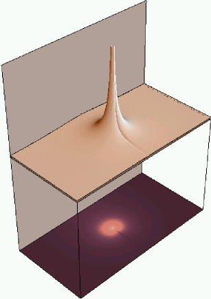
The picture for an $s$-wave superconductor is totally different. As shown in Fig. 2 the vortex has only little influence on the boundary density of states. Here, the high zero-energy density of states of the vortex rather illuminates the boundary. The small shadow on the right hand side of the vortex and the slight line between the vortex and the boundary is due to quasiparticles with an inclination angle of 90 degrees, that are trapped between the reflecting boundary and the potential step in the vortex core. Below, we will focus on a $d_{x^{2}-y^{2}}$-wave superconductor with an 110-boundary. More details of the $s$-wave superconductor and a $d$-wave superconductor with an arbitrary orientation of the boundary will be discussed in a following work.

Figure 2: Zero-energy local density of states of a $s$-wave superconductor. Again the reflecting boundary is situated at the back of the image, while the single Abrikosov vortex can be found at a distance of one coherence length $x_{V}=\xi$ in front of it. The high zero-energy density of states of the $s$-wave vortex slightly illuminates the boundary. An effective scattering parameter of $\delta=0.1\Delta_{0}$ has been used for the calculations.

In Fig. 3 we show the zero-energy density of states along the 110-boundary. The different curves correspond to different vortex positions $x_{V}$. The calculations have been done using a value of $\delta=0.1\Delta_{0}$. For increasing vortex to boundary distances $x_{V}$ we find a decrease of the shadow depth, while the width increases visibly. Apparently, the shadow effect exists for a wide range of vortex to boundary distances $x_{V}$ even larger than $10\xi$. For distances smaller than one coherence length $\xi$ a selfconsistent calculation of the pairing potential around the vortex might become necessary.

Figure 3: Zero-energy density of states of a $d_{x^{2}-y^{2}}$-wave superconductor along a 110-boundary for different vortex positions $x_{V}$. The curves are normalized to the local density of states at the boundary without vortex ($x_{V}\rightarrow\infty$). The effective scattering parameter is chosen to be $\delta=0.1\Delta_{0}$.

In the following we want to obtain a more detailed impression of the vortex shadow at the point $\mathcal{O}$. We also want to study the influence of the effective quasiparticle scattering parameter $\delta$ introduced in Eq. (5) on the local density of states. Without vortex, the value of the zero-energy density of states at the boundary shows a sensitive dependence on the decoherence parameter $\delta$. With decreasing $\delta$ the value of the zero-energy peak at the boundary increases rapidly. In Fig. 4 we show the zero-energy density of states at the point $\mathcal{O}$ as a function of the vortex to boundary distance $x_{V}$ for different values of $\delta$. The curves are normalized to the particular values of the zero-energy boundary density of states without a vortex or far away from the vortex center. We find that both the range and the relative depth of the shadow increase, if we decrease the scattering rate $\delta$. We want to point out, that this shadow effect can be observed in clean superconductors with a long mean free path as well as in superconductors with higher scattering rates.

Figure 4: Zero-energy quasiparticle density of states of a $d_{x^{2}-y^{2}}$-wave superconductor at the boundary as a function of the vortex position $x_{V}$. The different curves correspond to different mean free paths related to the inverse of $\delta$. The DOS of each curve is normalized on the corresponding boundary density of states without vortex.

In order to explain the suppression of the local zero-energy density of states at the surface, we now concentrate on a given point in the shadow region. In order to find the quasiparticle spectrum there, the angular integration in Eq. (5) has to be done. For each angle, the integrand corresponds to the contribution of a quasiparticle trajectory with the direction specified by $\theta$. Due to the phase gradient of the order parameter, the energy ”seen” by a quasiparticle flying along a trajectory is shifted. Additionally, this shift itself changes locally along the trajectory. Thus, for most of the angles, the Riccati-equations (Eq. (1)) are not evaluated at zero-energy. This is sufficient, however, to miss the sharp zero-energy peak of the bound state at the surface. As a consequence, the zero-energy density of states is reduced. In the quasiparticle spectrum the spectral weight of the bound states is shifted from the Fermi level towards higher energies. This effect is similar to the splitting of the zero-bias peak due to surface currents Fogelstroem .

Figure 5: Quasiparticle spectrum of a $d_{x^{2}-y^{2}}$-wave superconductor taken at a 110-boundary at the point adjacent to the vortex center ($\mathcal{O}$). The curves are calculated for different vortex distances $x_{V}$ from the boundary. The effective scattering parameter is chosen to be $\delta=0.1\Delta_{0}$.

In Fig. 5 we show the local density of states at the point $\mathcal{O}$ for different vortex to boundary distances $x_{V}$ as a function of energy. If the Abrikosov vortex is placed in the vicinity of the boundary we observe a distinct splitting of the zero-energy peak. With increasing distance between vortex and boundary the splitting is reduced. At $x_{V}=10\xi$ a splitting is no longer visible, while the height of the zero-energy peak is still considerably reduced.

The strong reduction of the zero-energy density of states at the 110-boundary of a $d_{x^{2}-y^{2}}$-superconductor has of course an important influence on the zero-bias anomaly in the tunneling conductance. Even in zero magnetic field vortices can remain in the high $T_{c}$-materials by pinning defects. In the vicinity of grain boundaries these pinned vortices will play an important role for the grain boundary tunneling due to the reduction of the zero-energy density of states. In a more detailed work we will also discuss the influence of a single vortex on the local density of states in the vicinity of a rough surface and we will consider several interesting boundary geometries apart from the flat surface.