Effective model of the electronic Griffiths phase

Abstract

We present simple analytical arguments explaining the universal emergence of electronic Griffiths phases as precursors of disorder-driven metal-insulator transitions in correlated electronic systems. A simple effective model is constructed and solved within Dynamical Mean Field Theory. It is shown to capture all the qualitative and even quantitative aspects of such Griffiths phases.

I Introduction

The recent discovery of a number of heavy fermion materials with non-Fermi liquid (NFL) thermodynamic and transport properties has been followed by a significant theoretical effort to understand the origin of the NFL behavior.G. R. Stewart (2001) In the cleaner systems, the proximity to a quantum critical point appears to dominate many of the observed properties.H. v. Löhneysen (1996); F. M. Grosche et al. (2000); J. A. Hertz (1976); T. Moryia (1985); M. A. Continentino et al. (1989); A. J. Millis (1993); P. Coleman et al. (2001); A. Schröder et al. (2000); Q. Si et al. (2001) In other heavy fermion systems disorder seems to play a more essential role and appears to be crucial for understanding the NFL behavior.O. O. Bernal et al. (1995); C. H. Booth et al. (1998); N. Büttgen et al. (2000); D. E. MacLaughlin et al. (2001, 2002); E. D. Bauer et al. (2002); C. H. Booth et al. (2002) Many experiments can be explained by the disordered Kondo model,O. O. Bernal et al. (1995) which has recently been put on a much stronger microscopical foundation.E. Miranda and V. Dobrosavljević (2001a, b); M. C. O. Aguiar et al. (2003)

The emergence of electronic Griffiths phases in models of correlated electrons has been establishedV. Dobrosavljević and G. Kotliar (1997); E. Miranda and V. Dobrosavljević (2001a, b); M. C. O. Aguiar et al. (2003) as a universal phenomenon, within a class of extended (“statistical”) Dynamical Mean Field Theory (DMFT) approaches.V. Dobrosavljević and G. Kotliar (1997) This statDMFT method provides an exact (numerical) treatment of localization in the absence of interactions, and reduces to the standard DMFT equationsA. Georges et al. (1996) in the absence of disorder. When both interactions and localization are present, non-Fermi liquid behavior emerges universally,E. Miranda and V. Dobrosavljević (2001a) as a precusor of a disorder-driven metal-insulator transition, due to a very broad distribution $P(T_{K})$ of local Kondo temperatures. This distribution has a low-$T_{K}$ tail of the form $P(T_{K})$ $\sim T_{K}^{\,\,\,\alpha-1}$, independent of the microscopic details or the specific form of disorder. The exponent $\alpha=\alpha(W)$ is found to be a smooth, monotonically decreasing function of the disorder strength $W$, and the NFL behavior emerges for $W$ greater than the critical value $W_{nfl}$ corresponding to $\alpha\leq 1$, when $P(T_{K})$ becomes singular at small $T_{K}$. As in other Griffiths phases, the thermodynamic and transport properties in this NFL region are dominated by rare events, which in this model correspond to sites with the lowest Kondo temperatures.

In this paper, we show that the same behavior is found in a simpler, standard DMFT version of the model with a judicious choice of bare disorder. We should emphasize that localization is not present in this effective model, but the Griffiths phase emerges in qualitatively the same fashion as in the above more realistic calculations. We discuss how the specific disorder distribution which is hand-picked in the effective model is dynamically generated by fluctuation effects within the statDMFT formulation, elucidating the origin of the universality of the Griffiths phase behavior. In addition, the simplicity of this DMFT effective model makes it possible to describe all the qualitative features of the solution using simple analytical arguments, thus eliminating the need for large scale numerical computations in the description of the electronic Griffiths phase. This may be crucial in order to address more complicated issues, such as the role of additional Ruderman-Kittel-Kasuya-Yosida (RKKY) interactions in disordered Kondo alloys.D. E. MacLaughlin et al. (2004)

This paper is organized as follows. Sec. II introduces the effective model for the electronic Griffiths phase as a DMFT model with a Gaussian distribution of random site energies. This model is solved analytically in the Kondo limit in Sec. III, and numerically in Sec. IV. The arguments explaining the universal aspects of the form of the renormalized disorder are presented in Sec. V. Sec. VI establishes a connection with the Griffiths phase in a single band Hubbard model, and Sec. VII contains our conclusions.

II Model

We consider the Anderson lattice model where the disorder is introduced by random site energies $\varepsilon_{i}$ in the conduction band, as given by the Hamiltonian

$$H = -t\sum_{\langle ij\rangle\sigma}(c_{i\sigma}^{\dagger}c_{j\sigma}+\mbox{H.c.})+\sum_{j\sigma}(\varepsilon_{j}-\mu)c_{j\sigma}^{\dagger}c_{j\sigma}$$ (1)

$$+V\sum_{j\sigma}\left(c_{j\sigma}^{\dagger}f_{j\sigma}+\mathrm{H}.\mathrm{c}.\right)+\sum_{j\sigma}E_{f}f_{j\sigma}^{\dagger}f_{j\sigma}$$

$$+U\sum_{j}f_{j\uparrow}^{\dagger}f_{j\uparrow}f_{j\downarrow}^{\dagger}f_{j\downarrow},$$

where $f_{j\sigma}$ and $c_{j\sigma}$ are annihilation operators for $f$- and conduction electrons, respectively. $V$ is the hybridization parameter, and $E_{f}$ is the $f$-electron energy. We assume $U\rightarrow\infty,$ and choose a Gaussian distribution of random site energies for the conduction band

$$P(\varepsilon_{i})=(2\pi W^{2})^{-1/2}\exp\{-\frac{1}{2}\varepsilon_{i}^{2}/W^{2}\}.$$ (2)

In Sec. V we will explain how this particular disorder distribution comes out naturally from the more generic statDMFT approach.

To solve these equations, we use the DMFT approach,A. Georges et al. (1996) which is formally exact in the limit of large coordination. We concentrate on a generic unit cell $j$, containing an $f$-site and its adjoining conduction electron Wannier state. After integrating out the conduction electron degrees of freedom, we obtain the effective action for the $f$-electron on site $j$

$$S_{imp}(j) = \sum_{\sigma}\int_{0}^{\beta}d\tau\int_{0}^{\beta}d\tau^{\prime}f_{j\sigma}^{\dagger}(\tau)\left[\delta(\tau-\tau^{\prime})(\partial_{\tau}+E_{f})\right.$$ (3)

$$+ \left.\Delta_{fj}(\tau-\tau^{\prime})\right]f_{j\sigma}(\tau^{\prime}).$$

Here, the restriction of no double $f$-site occupancy is implied. The hybridization function $\Delta_{fj}$ between the $f$-electron and the conduction bath $\Delta_{c}$ is given by

$$\Delta_{fj}(i\omega_{n})=\frac{V^{2}}{i\omega_{n}-\varepsilon_{j}+\mu-\Delta_{c}(i\omega_{n})}.$$ (4)

The self-consistency condition for the conduction bath (cavity field) assumes a simpler form for the semi-circular model density of statesA. Georges et al. (1996), which we use for simplicity. All the qualitative features of our solution are independent of the the form of the lattice, and the quantitative results depend only weakly on the details of the electronic band structure. For this model $\Delta_{c}(i\omega_{n})=t^{2}\overline{G_{c}}(i\omega_{n})$, where $\overline{G_{c}}(i\omega_{n})$ is the disorder-averaged Green’s function of the conduction electrons, and the self-consistency is enforced by

$$\overline{G_{c}}(i\omega_{n})=\langle[i\omega_{n}-\varepsilon_{j}+\mu-t^{2}\overline{G_{c}}(i\omega_{n})-\Phi_{j}(i\omega_{n})]^{-1}\rangle,$$ (5)

where

$$\Phi_{j}(i\omega_{n})=\frac{V^{2}}{i\omega_{n}-E_{f}-\Sigma_{fj}(i\omega_{n})},$$ (6)

and $\Sigma_{fj}$ is the $f$-electron self-energy derived from the impurity action of Eq. (3). From a technical point of view, within DMFT the solution of the disordered Anderson lattice problem reduces to solving an ensemble of a single impurity problems supplemented by a self-consistency condition.

We will solve the system of Eqs. (3)-(6) at zero temperature using the slave boson mean field theory approach.N. Read and D. M. Newns (1983); P. Coleman (1987) This approximation is knownE. Miranda and V. Dobrosavljević (2001a, b); M. C. O. Aguiar et al. (2003) to reproduce all the qualitative and even most of the accurately quantitative features of the exact DMFT solution at $T=0$. It introduces renormalization factors (quasi-particle weights) $Z_{j}$ and renormalized $f$-energy levels $\varepsilon_{fj}$, which are site-dependent quantities in the case of a disordered lattice. These parameters are determined by the saddle-point slave boson equations (see Ref. E. Miranda et al., 1996 for more details) which, on the real frequency axis, assume the form

$$-\frac{1}{\pi}\int_{-\infty}^{0}d\omega\,\mathrm{Im}\left[\frac{1}{\omega-\varepsilon_{fj}-Z_{j}\Delta_{fj}(\omega)}\right]=\frac{1}{2}(1-Z_{j}),$$ (7)

$$\frac{1}{\pi}\int_{-\infty}^{0}d\omega\,\mathrm{Im}\left[\frac{\Delta_{fj}(\omega)}{\omega-\varepsilon_{fj}-Z_{j}\Delta_{fj}(\omega)}\right]=\frac{1}{2}(\varepsilon_{fj}-E_{f}).$$ (8)

Eq. (6) in this case becomes

$$\Phi_{j}(\omega)=\frac{Z_{j}V^{2}}{\omega-\varepsilon_{fj}}.$$ (9)

III Analytical solution in the Kondo limit

Before presenting a numerical solution of the slave boson Eqs. (7)-(8) supplemented by the self-consistency condition of Eq. (5), we will solve these equations analytically in the Kondo limit for a given conduction bath. A comparison with the numerical solution will show that the self-consistency does not qualitatively change the analytical results.

The slave boson equations simplify in the Kondo limit $Z_{j}\rightarrow 0$. The integral in Eq. (7) is dominated by the low-frequency region, and the frequency dependence in $\Delta_{c}$ and $\Delta_{fj}$ can be neglected. Therefore, after integration

$$\varepsilon_{fj}\approx-Z_{j}\mathrm{Re}\left[\Delta_{fj}(0)\right],$$ (10)

where, for simplicity, we took a semi-circle conduction bath with $\mu=0$. In the integral of Eq. (8), the frequency dependence of $\Delta_{fj}$ can also be neglected. Introducing the energy cutoff $D$ and using Eq. (10) we obtain

$$Z_{j} \approx D\frac{\varepsilon_{j}^{2}+(\pi t^{2}\rho_{o})^{2}}{\pi t^{2}\rho_{o}V^{2}}e^{-\pi^{2}t^{2}\rho_{o}/J}e^{-\varepsilon_{j}^{2}/t^{2}\rho_{o}J}e^{\varepsilon_{j}/2t^{2}\rho_{o}}$$ (11)

$$= Z_{o}\frac{\varepsilon_{j}^{2}+(\pi t^{2}\rho_{o})^{2}}{(\pi t^{2}\rho_{o})^{2}}\exp\left[-\frac{\varepsilon_{j}^{2}}{t^{2}\rho_{o}J}\left(1-\frac{J}{2\varepsilon_{j}}\right)\right].$$

Here, $\rho_{o}$ is the density of states (DOS) of the conduction electrons at the Fermi level, $J=2V^{2}/|E_{f}|$, and $Z_{o}=Z\left(\varepsilon_{j}=0\right)$. The Kondo temperature is proportional to the quasi-particle weight, $T_{Kj}=\pi V^{2}\rho_{o}Z_{j}$. In the limit $\varepsilon_{j}\gg J/2$ and neglecting a weak site-energy dependence in the pre-factor, we obtain

$$T_{Kj}\approx T_{K}^{0}e^{-1/\lambda_{j}},$$ (12)

where the site dependent coupling constant is

$$\lambda_{j}=\frac{t^{2}\rho_{o}J}{\varepsilon_{j}^{2}},$$ (13)

and $T_{K}^{0}$ is the Kondo temperature in the clean limit (for $\varepsilon_{j}=0$). From these equations, we can immediately find the desired distribution of local Kondo temperatures $P(T_{K})=P(\varepsilon(T_{K}))|d\varepsilon/dT_{K}|$, which (up to a negligible logarithmic correction) is given asymptotically by

$$P(T_{K})\propto(T_{K}/T_{K}^{0})^{\alpha-1},$$ (14)

with

$$\alpha(W)=\frac{t^{2}\rho_{o}J}{2W^{2}}.$$ (15)

This expression is one of the central results of this paper. It has exactly the form expected for a Griffiths phase, where the exponent characterizing the local energy scale distribution assumes a parameter-dependent (tunable) form.

To show how the NFL behavior appears due to the singularity in $P(T_{K})$, we use the standard expression due to Wilson for the magnetic susceptibilityA. C. Hewson (1993)

$$\chi(T,T_{K})=\frac{C}{T+aT_{K}},$$ (16)

which is an excellent approximation for a single Kondo impurity. Here $C$ and $a$ are constants. In the disordered case, we can split the average susceptibility $\chi(T)=\int_{0}^{\infty}P(T_{K})\chi(T,T_{K})dT_{K}$ in a regular “bulk” part

$$\chi_{r}(T)=\int_{\Lambda}^{\infty}P(T_{K})\chi(T,T_{K})dT_{K},$$ (17)

and a potentially singular part

$$\chi_{s}(T)=C_{1}\int_{0}^{\Lambda}\frac{T_{K}^{\alpha-1}}{T+aT_{K}}dT_{K},$$ (18)

coming from the tail with low Kondo temperatures ($\Lambda$ is a crossover scale). At weak disorder, the exponent $\alpha$ is large and the distribution $P(T_{K})$ is regular, $\chi(0)=\chi_{o}+C_{2}/(\alpha-1)$, but NFL behavior emerges once $\alpha\leqslant 1$, which corresponds to

$$W\geq W_{nfl}=\sqrt{t^{2}\rho_{o}J/2}.$$ (19)

For $\alpha=1$ the magnetic susceptibility has a logarithmic divergence, $\chi(T)\propto\ln(1/T)$, characteristic of marginal Fermi liquid behavior,C. M. Varma et al. (1989) while for $\alpha<1$ a power law divergence is obtained, $\chi(T)\propto T^{\alpha-1}$ as $T\rightarrow 0$. The same singularity also leads to an anomalous behavior in the transport properties, as shown in detail in Refs. E. Miranda et al., 1996 and E. Miranda et al., 1997.

IV Numerical results

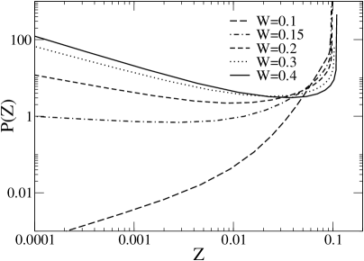
Figure 1: Distribution of the local Kondo temperatures. The disorder ranges from moderate $W=0.1$ to strong $W=0.4$. We used $V=0.5$, $E_{f}=-1$, and $\mu=-0.1$.

In the above derivation we ignored the fact that the conduction bath $\Delta_{c}$ has to be self-consistently determined. This will also produce particle-hole asymmetry and an asymmetric distribution of Kondo temperatures $T_{Kj}$. A nonzero chemical potential will further increase this asymmetry. However, the numerical solution we obtained using the slave boson approximation at zero temperature shows that the essential physics described by Eqs. (12)-(15) remains qualitatively correct. The distribution of local Kondo temperatures in the asymptotic limit is indeed a power law, $P(T_{K})\sim T_{K}\,\!^{\alpha-1}$, where the exponent $\alpha$ is a decreasing function of disorder.

Fig. 1 shows the distribution $P(T_{K})$ for several values of the disorder distribution strength $W$. For the parameters that we here use, the system is close to the Kondo limit, and the Kondo gap of the clean system is approximately 0.04 (in energy units of the half bandwidth of bare DOS). The NFL behavior appears for $W\gtrsim 0.14$. We note that in the NFL regime the power law behavior appears already for the site energies $\varepsilon_{j}$ which deviate only moderately from the mean (zero) value. In other words, the asymptotic behavior is established well before we attain very rare realizations of $\varepsilon_{j}$ which belong to the tail of the Gaussian distribution. For example, for $W=0.3$, sites with $\varepsilon_{j}\gtrsim 0.4$ (which correspond to $Z\lesssim 0.01$) are already in the power-law regime.

Figure 2: Inverse power law parameter $\alpha^{-1}$ as a function of $W^{2}$. For weak and moderate disorder this dependence is linear. Here $V=0.5$, $E_{f}=-1$, and $\mu=-0.2$.

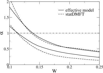
Figure 3: Power law exponent $\alpha$ as a function of disorder strength measured by the standard deviation $W$. Full lines are the effective model results, and dashed lines are the statDMFT results. The hybridization $V$ is taken to be 0.5 and $E_{f}=-1$. The chemical potential is $\mu=-0.1$ (upper lines), and $-0.5$ (lower lines). The onset of NFL behavior occurs at $\alpha=1$.

According to the simplified derivation from Sec III, the exponent $\alpha$ is inversely proportional to $W^{2}$. The numerical results shown in Fig. 2 confirm such behavior for weak and moderate disorder. For strong disorder there appear some deviations from this formula, which can be ascribed to the dependence of the DOS at the Fermi level on the disorder strength.

Before we present arguments which justify our effective DMFT model approach, let us make a direct comparison with the statDMFT results from Ref. M. C. O. Aguiar et al., 2003. In this approach, very broad distributions of local Kondo temperatures are generated for arbitrary distributions of bare disorder. In particular, even if the bare distribution is bounded, sites with arbitrarily small Kondo temperatures will exist, and their distribution will have a power law tail. This is a consequence of the spatial fluctuations of the conduction electron cavity field, as we discuss in detail in the next Section. In Fig. 3 we compare the values of the exponent $\alpha$ for the effective model with Gaussian disorder of variance $W^{2}$, and the statDMFT results obtained for a bounded uniform distribution of bare disorder with the same variance. Remarkably, not only does the electronic Griffiths phase emerge in the same fashion, but the numerical values of disorder strength determining the onset of NFL behavior are also almost the same. The comparison is made for two different values of the chemical potential. As we move further away from half-filling by changing the chemical potential, the critical value $W_{nfl}$ decreases. That is expected since $\alpha$ should be proportional to the bare (noninteracting) DOS at the Fermi level.

V The role of spatial fluctuations and the form of renormalized disorder

In this Section we explain the universal aspects of the emergence of the electronic Griffiths phase within the more generic statistical DMFT. In particular, we show how the Gaussian tails in the distribution of renormalized disorder appear for an arbitrary form of the bare disorder. Moreover, we present arguments showing that the Griffiths phase appears generically as a precursor of the Mott-Anderson metal-insulator transition.

V.1 Universality of the renormalized disorder distribution

In the above DMFT formulation, we had to choose a special form of disorder distribution in order to obtain the desired power-law distribution of Kondo temperatures. Had we chosen a different distribution, the results would not have held. For example, for a bounded distribution of site energies, there would always be a minimum value of the Kondo temperature, and thus no power-law tail. On the other hand, from numerical simulations of lattices with finite coordination, it has been established that the emergence of the Griffiths phase is a universal phenomenon.M. C. O. Aguiar et al. (2003) Why? To understand the reason for this, we note that for finite coordination (as opposed to the DMFT limit) the cavity bath $\Delta_{c}$ is not self-averaging, but is a site-dependent, random quantity $\Delta_{cj}$. In this statDMFT formulation, the local conduction electron Green’s function is given by

$$G_{cj}(i\omega_{n})=\frac{1}{i\omega_{n}-\varepsilon_{j}+\mu-\Delta_{cj}(i\omega_{n})-\Phi_{j}(i\omega_{n})},$$ (20)

where $\Phi_{j}$ describes the local scattering of the conduction electrons off the $f$-shell at site $j$, and is given as before by Eq. (6).

For weak disorder, the corresponding fluctuations are small, and we can separate

$$\Delta_{cj}=\Delta_{c}^{av}+\delta\Delta_{cj}.$$ (21)

In the following, we compute the distribution function for the fluctuations of the cavity field, which will lead to the renormalized form of the disorder distribution function. The renormalized site energies can be defined as

$$\widetilde{\varepsilon}_{j}=\varepsilon_{j}+\delta\Delta_{cj}^{R},$$ (22)

where $\delta\Delta_{cj}^{R}=\mathrm{Re}\left[\delta\Delta_{cj}(\omega=0)\right]$. We stress that the cavity fluctuations are present for a general finite coordination electronic system in the presence of disorder of any kind. In particular, the disorder in hybridization parameters $V_{j}$, or local $f$-energy levels $E_{fj}$, will induce fluctuations in the local DOS even if random site energies $\varepsilon_{j}$ in the conduction band are absent. Furthermore, as we argue in the next subsection, the renormalized distribution $P(\widetilde{\varepsilon}_{j})$ will have universal Gaussian tails even if the bare distribution $P(\varepsilon_{j})$ is bounded. Note that $\delta\Delta_{cj}$ has a real as well as an imaginary part $\delta\Delta_{cj}^{I}$, due to the fact that fluctuations locally violate particle-hole symmetry. However, we show in the Appendix that $\delta\Delta_{cj}^{I}$ fluctuations, at least when treated to leading order, do not produce singular behavior in $P(T_{K})$ and therefore can be neglected when examining the emergence of the electronic Griffiths phase.

V.2 The Gaussian nature of the renormalized distribution

From detailed numerical studies it has become clear that the onset of the Griffiths phase in disordered Anderson lattices generally occurs already for a relatively moderate amount of disorder. In this limit, the relevant distributions are determined essentially by the central limit theorem, therefore resulting in a Gaussian form of the tails for $P(\widetilde{\varepsilon}_{j})$. This is precisely what is needed to justify the DMFT effective model, where such Gaussian tails are assumed from the outset.

Before engaging in more precise computations of these distributions, it is worth pausing to comment on the physical validity of the assumed Gaussian statistics, i.e. the relevance of the central limit theorem in the cases of interest. Quite generally, if a certain quantity can be represented as a sum of a large number of independent random variables, then the central limit theorem tells us that the resulting distribution will be Gaussian, irrespective of the specific form of the distributions of the individual terms in the sum. In our case, the fluctuations of the local cavity field result from Friedel oscillations of the electronic wave functions, induced by other impurities which may lie at a relatively long distance from the given site. This is a result of the slow ($\sim R^{-d}$) decay of the amplitude of the Friedel oscillations in $d$ dimensions, where $R$ is the distance from the impurity site. The situation is very reminiscent of the Weiss molecular field of an itinerant magnet, where the RKKY spin-spin interactions have a long range character for the very same reason, being as they are a reflection of similar Friedel oscillations. Furthermore, as we will explicitly show, the leading corrections (to order $\mathcal{O}\left(W^{2}\right)$) at weak disorder take the form of a linear superposition of contributions from single impurity scatterers, and thus of a sum of independent random numbers, for which we expect the central limit theorem to hold.

To obtain the precise form of this distribution, it therefore suffices to compute the variance

$$\sigma_{R}^{2}=\left\langle(\delta\Delta_{cj}^{R})^{2}\right\rangle,$$ (23)

to leading order in disorder strength. To compute the fluctuations $\delta\Delta_{cj}$ at weak disorder, we note that the cavity field $\Delta_{cj}$ can be computed if we consider a particular site with $\varepsilon_{j}=0$ (call it site $0$), and compute its Green’s function in a random medium. At zero frequency for this site

$$\Delta_{co}=\mu-1/G_{oo}.$$ (24)

The corresponding variation is

$$\delta\Delta_{co}=\delta G_{oo}/(G_{oo})^{2}.$$ (25)

We still need to compute the fluctuation $\delta G_{oo},$ which can be expanded in powers of the random potential $\varepsilon_{j}$. In doing this, we have ignored the interaction renormalizations of the random potential for conduction electrons. We will return to re-examine this effect in the Appendix. Note, however, that in the absence of interactions in the environment of a given site, the following expressions provide the exact leading contributions at weak disorder.

To leading order, we can write

$$\delta G_{oo}=\sum\limits_{j}\varepsilon_{j}(G_{oj})^{2}+\mathcal{O}(\varepsilon^{2}).$$ (26)

This gives

$$\sigma_{R}^{2}=CW^{2}+\mathcal{O}(W^{4}),$$ (27)

where

$$C=\sum\limits_{\genfrac{}{}{0.0pt}{2}{j}{(j\neq 0)}}\left[\mathrm{Re}\frac{(G_{oj})^{2}}{(G_{oo})^{2}}\right]^{2}.$$ (28)

The Green’s function sum $C$ will numerically depend on the lattice geometry, but will generally be a dimensionless number of order one.

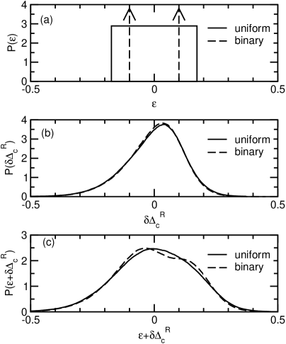
Figure 4: StatDMFT results for the disorder distributions. Universal Gaussian-like tails appear in the cavity field fluctuations, panel (b), and the renormalized disorder distributions, panel (c), even though the bare disorder distributions are bounded (uniform and binary), panel (a). We used $V=0.5$, $E_{f}=-1$, and $\mu=-0.5$.

The distribution of renormalized disorder $\widetilde{\varepsilon}=\varepsilon+\delta\Delta_{c}^{R}$ is given by a convolution of the distributions $P_{1}(\varepsilon)$ and $P_{2}(\delta\Delta_{c}^{R})$

$$P(\widetilde{\varepsilon})=\int_{-\infty}^{\infty}d\omega\,P_{1}(\widetilde{\varepsilon}-\omega)P_{2}(\omega).$$ (29)

If the bare distribution is bounded, (e.g. a standard “box” distribution), then Gaussian tails will emerge due to the fluctuations in $\delta\Delta_{c}^{R}$, and the “size” of the tails will be determined by an effective disorder corresponding to $W_{eff}^{(0)}=W\sqrt{C}$. Here, the superscript ⁽⁰⁾ indicates that we ignored the interaction renormalizations. In the Appendix, we argue that the effective scattering potentials $\Phi_{j}$ will further renormalize the disorder distribution, but the Gaussian tails will remain as its generic feature.

Figure 5: StatDMFT results for the distribution of Kondo temperatures for uniform and binary bare disorder distributions (upper panel). The lower panel shows the exponent $\alpha$ as a function of disorder strength. The results are qualitatively the same regardless of the specific form of the disorder distribution. We used $V=0.5$, $E_{f}=-1$, and $\mu=-0.5$.

Now we present numerical results which provide strong evidence for the universality of the renormalized disorder. Fig. 4 shows the results obtained within the statDMFTE. Miranda and V. Dobrosavljević (2001a) for uniform and binary disorder distributions with the same standard deviation $W=0.1$. As anticipated by Eq. (27), the fluctuations of the cavity bath acquire an approximately Gaussian form with the same variance for both bare disorder distributions, panel (b). The renormalized disorder distribution $P(\widetilde{\varepsilon})$ exhibits long tails, panel (c), although the bare distributions are bounded, panel (a). These Gaussian-like tails are the main universal feature of the renormalized disorder, and they are crucial for the appearance of the singular behavior in $P(T_{K})$ which leads to the formation of the Griffiths phase.

StatDMFT results in Fig. 5 provide further illustration of the universality. The upper panel shows that the distributions of Kondo temperatures for uniform and binary bare disorder distributions with the same standard deviation $W$ are qualitatively the same. The exponent $\alpha$, which determines the slope of the distribution tails, is shown at the lower panel as a function of $W$. It depends very weakly on the particular form of disorder distribution.

V.3 Localization effects

In the strict DMFT formulation $\alpha\approx t^{2}\rho_{o}J/2W^{2}$, where $\rho_{o}\equiv\rho_{av}$ is simply the (algebraic) average DOS of the conduction electrons, which therefore remains finite even at the localization transition.P. W. Anderson (1958) If $J$ is chosen to be large enough, the above seems to suggest that the Griffiths phase may not emerge before the electrons localize at $W=W_{c}\sim 1/\rho_{av}$. However, in a theory that includes localization, the Kondo spins do not see the average, but rather the typical DOS of the conduction electrons.V. Dobrosavljević and G. Kotliar (1997); Dobrosavljević et al. (2003) Thus, in the NFL criterion, Eq. (19), one should actually replace $\rho_{o}\rightarrow\rho_{typ}$, a quantity that becomes very small (and eventually vanishes) as the Anderson transition is approached, viz.

$$\rho_{typ}=A(W_{c}-W)^{\beta},$$ (30)

where $A$ and $\beta$ are constants. We thus get

$$W_{nfl}^{2}=\frac{1}{2}At^{2}J(W_{c}-W_{nfl})^{\beta}.$$ (31)

This transcendental equation cannot be solved in closed form in general, but an approximate solution can be found for $W_{c}^{2-\beta}/At^{2}J\ll 1$. In this case, the quantity $\delta W=1-W_{nfl}/W_{c}$ will be small, and to leading order in $\delta W$

$$W_{nfl}=W_{c}-(At^{2}J/2)^{-1/\beta}W_{c}^{2/\beta}<W_{c}.$$ (32)

Therefore, the Griffiths phase emerges strictly before the transition is reached.

VI Electronic Griffiths phase in the vicinity of the metal-insulator transition

Previous workV. Dobrosavljević and G. Kotliar (1997) has shown that the electronic Griffiths phase appears also in a single band Hubbard model, as a precursor to the Mott-Anderson metal-insulator transition (MIT). Since the Hubbard model at half-filling is equivalent to the charge-transfer modelJ. Zaanen et al. (1985) of the MIT, we examine in this Section the appearance of the Griffiths phase within this model, which can be considered a version of the Anderson lattice model that we examined in our approach.

The charge transfer model has been used to describe the Mott metal-insulator transition for various systems, including copper oxides.F. C. Zhang and T. M. Rice (1988) It consists of a two band model, where one of the bands is narrow, and has large on-site interaction $U$ (Copper $d$-band), while the other band is broad enough that electron-electron interactions can be neglected (Oxygen $p$-band). A disordered version of this model is also appropriate to describe the Mott-Anderson transitionV. Dobrosavljević and G. Kotliar (1997) in doped semiconductors such as Si:P. Here, the narrow band correspondsB. I. Shklovskii and A. L. Efros (1984) to the impurity band of the Phosphorus donors, while the broad one is the conduction band of Silicon. This model is given exactly by the Hamiltonian of Eq. (1), but supplemented by the constraint

$$\overline{n_{fj}}+\overline{n_{cj}}=1,$$ (33)

which can be enforced by adjusting the value of the chemical potential. Here $n_{fj}$ and $n_{cj}$ are the average number of conduction and $f$-electrons on site $j$, and the overbar denotes the average over disorder. In the mean field slave boson approach, the average occupancy of the $f$-site is equal to

$$n_{fj}=1-Z_{j}.$$ (34)

As the $f$-electron energy level is decreased ($|E_{f}|$ increased), the occupancy of the $f$-sites becomes larger: the charge is “transferred” from the conduction band. The transition to the Mott insulator is found for sufficiently large $|E_{f}|$. At least within DMFT, this metal-insulator transition has the same character as the more familiar Mott transition in a single band Hubbard model. As an illustration, we show on Fig. 6 the number of conduction electrons per site, $n_{c}=Z$, as a function of $E_{f}$, in the clean limit.

Figure 6: Number of conduction electrons per site as a function of the $f$-level energy $E_{f}$. The approach to the insulating phase is linear, $n_{c}\sim E_{f}-E_{f}^{c}$, where $E_{f}^{c}$ is the critical value for the $f$-level energy. The hybridization $V=0.5$, and $E_{f}$ is measured with respect to the middle of the conduction band.

We have solved our effective model in the parameter regime relevant to the approach to the Mott-Anderson transition, and the results demonstrate the emergence of an electronic Griffiths phase in the same fashion as for the Anderson lattice model, consistent with statDMFT results.V. Dobrosavljević and G. Kotliar (1997). Here, the $f$-level energy in Fig. 7 is measured with respect to the middle of the conduction band, and not with respect to the chemical potential as in Sec. IV. For the parameters used in Fig. 7, the system is in the mixed valence regime, not in the Kondo limit, and stronger disorder is needed for the appearance of the NFL electronic Griffiths phase, again in close agreement with statDMFT results.V. Dobrosavljević and G. Kotliar (1997) These results demonstrate that our effective model proves capable to describe the emergence of the electronic Griffiths phase as a universal phenomenon in correlated electronic systems with disorder.

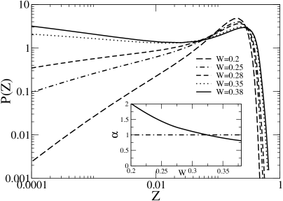
Figure 7: Distribution of local Kondo temperatures for several levels of disorder. The total number of electrons per unit cell is fixed to 1. The disorder ranges from $W=0.2$ to $0.38$. We used $V=0.5$ and $E_{f}=-1.3$, where $E_{f}$ is measured with respect to the middle of the conduction band. The inset shows the exponent $\alpha$ as a function of the disorder strength. The NFL phase occurs for $\alpha\leq 1$.

VII Summary and outlook

In this paper we have identified an analytically solvable infinite range model, which captures the emergence of electronic Griffiths phases found within the more generic statDMFT approaches.E. Miranda and V. Dobrosavljević (2001a); M. C. O. Aguiar et al. (2003); V. Dobrosavljević and G. Kotliar (1997) In this effective model, a specific distribution of disorder is postulated, leading to a power-law distribution of local Kondo temperatures and NFL behavior for sufficiently strong disorder. We have also presented arguments explaining how this specific form of randomness is universally generated by renormalizations due to disorder-induced fluctuations of the conduction bath. In this sense our effective model can be regarded as a (stable) fixed point theory of electronic Griffiths phases.

The main motivation for introducing this effective model lies in its simplicity, allowing an analytical solution, and thus providing further insight into the mechanism for the emergence of the electronic Griffiths phase. Nevertheless, an essential ingredient is still missing from our Griffiths phase theory, namely the inter-site RKKY interactions between Kondo spins. According to the existing picture, all the spins with $T_{K}<T$ will not be Kondo screened, thus providing a large contribution to thermodynamic response. These decoupled spins will, however, not act as free local moments, but will feature dynamics dominated by frustrating inter-site RKKY interactions. Recent experiments on disordered Kondo alloys indeed seem to suggest the presence of low temperature glassy dynamics with a negligible freezing temperature.D. E. MacLaughlin et al. (2001, 2004) The simplifications introduced by our effective model open an attractive avenue to incorporate both the Kondo effect and the RKKY interaction in a single theory. This fascinating direction remains a challenge for future work.

Appendix A Fluctuations in $\delta\Delta_{cj}^{I}$

In Sec. V we have ignored the fluctuations in the imaginary part of the cavity function $\delta\Delta_{cj}^{I}.$ The corresponding contribution to the low-$T_{K}$ tail is sub-leading, as we now show. We need to focus on rare events that produce exceptionally small values of the local conduction electron DOS $\rho_{j}=-\frac{1}{\pi}G_{cj}(0)$. Using Eq. (20), and ignoring the fluctuations in $\delta\Delta_{cj}^{R}$, we see that low values for $\rho_{j}$ correspond to exceptionally high values for $\delta\Delta_{cj}^{I}.$ We therefore need to compute the form of the high-$\delta\Delta_{cj}^{I}$ tail of $P(\delta\Delta_{cj}^{I}).$ Just as for the real part, we can estimate the fluctuations of $\delta\Delta_{cj}^{I}$ by calculating the second moment,

$$\sigma_{I}^{2}=\left\langle(\delta\Delta_{cj}^{I})^{2}\right\rangle,$$ (35)

and we get

$$\sigma_{I}^{2}=C_{I}W^{2}+O(W^{4}),$$ (36)

where

$$C_{I}=\sum\limits_{\genfrac{}{}{0.0pt}{2}{j}{(j\neq 0)}}\left[\operatorname{Im}\frac{(G_{oj})^{2}}{(G_{oo})^{2}}\right]^{2}.$$ (37)

In this approximation, the quantity $\delta\Delta_{cj}^{I}$ has a Gaussian distribution, and we find

$$P(T_{K})\sim T_{K}^{-1}\exp\left\{-\frac{J^{2}}{2\pi^{2}\sigma_{I}^{2}}\ln^{2}(D/T_{K})\right\}.$$ (38)

As we can see, because the “log” in the exponent has an extra power of two, this distribution is log-normal and not power-law. Therefore the $\delta\Delta_{cj}^{I}$ fluctuations, at least when treated on the Gaussian level as we have done, do not lead to a singular $P(T_{K})$ distribution. Thus, to leading order we can ignore these fluctuations when examining the emergence of the electronic Griffiths phase.

Appendix B Interaction renormalizations

In these estimates, we have omitted an important ingredient, the fact that Kondo disorder itself will produce additional scattering, i.e. disorder in the conduction channel, which needs to be self-consistently determined. As we have shown in previous work,E. Miranda and V. Dobrosavljević (2001a) this results in a distribution of effective scattering potentials $\Phi_{j}$, corresponding to the Kondo spins (note that in the uniform case, the $\Phi_{j}$-s are the same on all sites, resulting in no scattering, but contributing to the formation of the Kondo gap). The resulting scattering, in the weak disorder limit again can be considered as a Gaussian distributed potential of width

$$W_{\Phi}=\left\langle\Phi_{j}^{2}\right\rangle^{1/2}.$$ (39)

Note however that this additional “Kondo” scattering does not enter directly (at site $0$) in the solution of the local Kondo problem, since the local f-site “sees” the corresponding c-site with the f-site removed. However, the presence of $\Phi_{j}$-s on all other sites $(j\neq 0)$ does modify the form of $\delta\Delta_{cj}^{R}$ which, therefore, has to be computed by including this additional scattering. At weak disorder, we expect

$$\left\langle\Phi_{i}^{2}\right\rangle=C_{1}W_{eff}^{2},$$ (40)

where the constant $C_{1}$ measures the response of the Kondo spins to the hybridization disorder. Note that $W_{eff}$ enters here, since the $\Phi_{j}$-s are obtained from the solution of local Kondo problems, which are determined by the strength of the renormalized site disorder, as modified by hybridization fluctuations. We therefore need to compute $W_{eff}$ self-consistently, and we get

$$W_{eff}^{2}=W^{2}+C(W^{2}+C_{2}W_{eff}^{2}),$$ (41)

or

$$W_{eff}=\sqrt{\frac{1+C}{1-CC_{2}}}W.$$ (42)

This reasoning, valid for weak bare disorder illustrates how the effective disorder is generated in the conduction band even if it originally was not there, or is enhanced due to additional Kondo scattering, if already present. In addition, these arguments illustrate how Gaussian tails are generated for the renormalized disorder, even if they are not introduced in the bare model. Of course, nonlinear effects at stronger disorder cannot be accounted for in this simple fashion, which is especially true for the consideration of the additional scattering introduced by disordered Kondo spins. Nevertheless, the simple arguments that we presented illustrate how universality is produced by renormalizations due to cavity field fluctuations, and seem to capture the essential features of the emergence of the electronic Griffiths phase.

References

- G. R. Stewart (2001) G. R. Stewart, Rev. Mod. Phys. 73, 797 (2001).
- H. v. Löhneysen (1996) H. v. Löhneysen, J. Phys.: Condens. Matter 8, 9689 (1996).
- F. M. Grosche et al. (2000) F. M. Grosche, P. Agarwal, S. R. Julian, N. J. Wilson, R. K. W. Haselwimmer, S. J. S. Lister, N. D. Mathur, F. V. Carter, S. S. Saxena, and G. G. Lonzarich, J. Phys.: Condens. Matter 12, L533 (2000).
- J. A. Hertz (1976) J. A. Hertz, Phys. Rev. B 14, 1165 (1976).
- T. Moryia (1985) T. Moryia, Spin Fluctuations in Itinerant Electron Magnetism (Springer-Verlag, Berlin, 1985).
- M. A. Continentino et al. (1989) M. A. Continentino, G. M. Japiassu, and A. Troper, Phys. Rev. B 39, 9734 (1989).
- A. J. Millis (1993) A. J. Millis, Phys. Rev. B 48, 7183 (1993).
- P. Coleman et al. (2001) P. Coleman, C. Pépin, Q. Si, and R. Ramazashvili, J. Phys.: Condens. Matter 13, R723 (2001).
- A. Schröder et al. (2000) A. Schröder, G. Aeppli, R. Coldea, M. Adams, O. Stockert, H.v. Löhneysen, E. Bucher, R. Ramazashvili, and P. Coleman, Nature 407, 351 (2000).
- Q. Si et al. (2001) Q. Si, S. Rabello, K. Ingersent, and J. L. Smith, Nature 413, 804 (2001).
- O. O. Bernal et al. (1995) O. O. Bernal, D. E. MacLaughlin, H. G. Lukefahr, and B. Andraka, Phys. Rev. Lett. 75, 2023 (1995).
- C. H. Booth et al. (1998) C. H. Booth, D. E. MacLaughlin, R. H. Heffner, R. Chau, M. B. Maple, and G. H. Kwei, Phys. Rev. Lett. 81, 3960 (1998).
- N. Büttgen et al. (2000) N. Büttgen, W. Trinkl, J.-E. Weber, J. Hemberger, A. Loidl, and S. Kehrein, Phys. Rev. B 62, 11545 (2000).
- D. E. MacLaughlin et al. (2001) D. E. MacLaughlin, O. O. Bernal, R. H. Heffner, G. J. Nieuwenhuys, M. S. Rose, J. E. Sonier, B. Andraka, R. Chau, and M. B. Maple, Phys. Rev. Lett. 87, 066402 (2001).
- D. E. MacLaughlin et al. (2002) D. E. MacLaughlin, O. O. Bernal, J. E. Sonier, R. H. Heffner, T. Taniguchi, and Y. Miyako, Phys. Rev. B 65, 184401 (2002).
- E. D. Bauer et al. (2002) E. D. Bauer, C. H. Booth, G. H. Kwei, R. Chau, and M. B. Maple, Phys. Rev. B 65, 245114 (2002).
- C. H. Booth et al. (2002) C. H. Booth, E.-W. Scheidt, U. Killer, A. Weber, and S. Kehrein, Phys. Rev. B 66, 140402 (2002).
- E. Miranda and V. Dobrosavljević (2001a) E. Miranda and V. Dobrosavljević, Phys. Rev. Lett. 86, 264 (2001a).
- E. Miranda and V. Dobrosavljević (2001b) E. Miranda and V. Dobrosavljević, J. Magn. Magn. Mat. 226-230, 110 (2001b).
- M. C. O. Aguiar et al. (2003) M. C. O. Aguiar, E. Miranda, and V. Dobrosavljević, Phys. Rev. B 68, 125104 (2003).
- V. Dobrosavljević and G. Kotliar (1997) V. Dobrosavljević and G. Kotliar, Phys. Rev. Lett. 78, 3943 (1997).
- A. Georges et al. (1996) A. Georges, G. Kotliar, W. Krauth, and M. J. Rozenberg, Rev. Mod. Phys. 68, 13 (1996).
- D. E. MacLaughlin et al. (2004) D. E. MacLaughlin, R. H. Heffner, O. O. Bernal, K. Ishida, J. E. Sonier, G. J. Nieuwenhuys, M. B. Maple, and G. R. Stewart, J. Phys.:Condens. Matter 16, S4479 (2004) (2004).
- N. Read and D. M. Newns (1983) N. Read and D. M. Newns, J. Phys. C 16, L1055 (1983).
- P. Coleman (1987) P. Coleman, Phys. Rev. B 35, 5072 (1987).
- E. Miranda et al. (1996) E. Miranda, V. Dobrosavljević, and G. Kotliar, J. Phys.: Condens. Matter 8, 9871 (1996).
- A. C. Hewson (1993) A. C. Hewson, The Kondo Problem to Heavy Fermions (Cambrige University Press, Cambridge, 1993).
- C. M. Varma et al. (1989) C. M. Varma, P. B. Littlewood, S. Schmitt-Rink, E. Abrahams, and A. E. Ruckenstein, Phys. Rev. Lett. 63, 1996 (1989).
- E. Miranda et al. (1997) E. Miranda, V. Dobrosavljević, and G. Kotliar, Phys. Rev. Lett. 78, 290 (1997).
- P. W. Anderson (1958) P. W. Anderson, Phys. Rev. 109, 1492 (1958).
- Dobrosavljević et al. (2003) V. Dobrosavljević, A. A. Pastor, and B. K. Nikolić, Europhys. Lett. 62, 76 (2003).
- J. Zaanen et al. (1985) J. Zaanen, G. A. Sawatzky, and J. W. Allen, Phys. Rev. Lett. 55, 418 (1985).
- F. C. Zhang and T. M. Rice (1988) F. C. Zhang and T. M. Rice, Phys. Rev. B 37, 3759 (1988).
- B. I. Shklovskii and A. L. Efros (1984) B. I. Shklovskii and A. L. Efros, Electronic Properties of Doped Semiconductors (Springer-Verlag, Berlin, 1984).