Electron Spectral Functions of Reconstructed Quantum Hall Edges

Abstract

During the reconstruction of the edge of a quantum Hall liquid, Coulomb interaction energy is lowered through the change in the structure of the edge. We use theory developed earlier by one of the authors [K. Yang, Phys. Rev. Lett. 91, 036802 (2003)] to calculate the electron spectral functions of a reconstructed edge, and study the consequences of the edge reconstruction for the momentum-resolved tunneling into the edge. It is found that additional excitation modes that appear after the reconstruction produce distinct features in the energy and momentum dependence of the spectral function, which can be used to detect the presence of edge reconstruction.

The paradigm of the Quantum Hall effect (QHE) edge physics is based on an argument due to Wen, Wen according to which the low-energy edge excitations are described by a chiral Luttinger liquid (CLL) theory. One attractive feature of this theory is that due to the chirality, the interaction parameter of the CLL is often tied to the robust topological properties of the bulk and is independent of the details of electron interaction and edge confining potential; studying the physics at the edge thus offers an important probe of the bulk physics. It turns out, however, that the CLL ground state may not always be stable. MacDonald-Yang-Johnson ; Chamon-Wen On the microscopic level, the instability is driven by Coulomb interactions and leads to the change of the structure of the edge. This effect has been termed “edge reconstruction”. One of its manifestations is the appearance of new low-energy excitations of the edge not present in the original CLL theory.

Based on the insight from numerical studies of the edge reconstruction, Wan-Yang-Rezayi ; Wan-Rezayi-Yang a field-theoretic description of the effect has been proposed by one of us. Yang Remarkably, it provides an explicit expression for the electron operator in terms of the fields that describe the low-energy edge excitations after the reconstruction. This allows one to calculate many observable quantities. In this paper, we describe the calculation of the spectral function of the electron in the reconstructed edge. This function can be probed in tunneling experiments where the electron’s momentum parallel to the edge is conserved (the so-called momentum-resolved tunneling). Experiments of this kind are currently being performed. Kang ; Grayson It has also been proposed that momentum-resolved tunneling may be used to detect the multiple branches of edge excitations of hierarchy states. Zulicke-Shimshoni-Governale

Our results show that the appearance of the new edge excitations after the reconstruction modifies the electron spectral function qualitatively. It leads to the redistribution of the spectral weight away from the peak corresponding to the original edge mode, and produces singularities corresponding to the new edge modes. For simplicity we have focused on the principal Laughlin sequence, although generalization to the hierarchy states should be straightforward. We also propose a particular experimental setup that involves momentum-resolved electron tunneling which is ideal for detecting possible edge reconstruction.

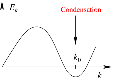
Figure 1: The spectrum of the edge excitations after the reconstruction has a minimum below 0. Excitations with momenta near $k_{0}$ are condensed.

Previous numerical studies Wan-Rezayi-Yang have suggested that the phenomenon of edge reconstruction can be understood as an instability of the original edge mode described by the CLL theory. This instability occurs as a result of increasing curvature of the edge spectrum as the edge confining potential softens. The spectrum curves down at high values of momenta until it touches zero at the transition point (see Fig. 1). This signals an instability of the ground state as the edge excitations begin to condense at finite momentum $k_{0}$. Such condensation implies the appearance of a bump in the electron density localized in real space at $y_{0}=l^{2}k_{0}$, where $y_{0}$ is the coordinate normal to the edge and $l$ is the magnetic length. These condensed excitations form a superfluid (with power-law correlation) which possesses a neutral “sound” mode that can propagate in both directions.

The CLL scenario outlined above is relevant to the case of sharp edge confining potential. In the opposite limit of soft confining potential, the description of the edge in terms of intermittent compressible and incompressible stripes has been developed by Chklovskii et al. Chklovskii In the same limit, emergence of new edge excitation modes was predicted. Aleiner ; Balev We believe that the description of the crossover between the two limits should be possible by extending the present scenario to multiple edge reconstruction transitions, each characterized by a different momentum $k_{i}$, at which the instabilities occur. We comment on this possibility throughout the text.

Following Ref. Yang, , we introduce two slowly varying fields $\phi_{1}$ and $\varphi$ which describe the original charged edge mode and the pair of the two new neutral modes, respectively. The total action of the reconstructed edge of the FQHE at filling fraction $\nu=1/m$ is: $S=S_{1}+S_{\varphi}+S_{\rm int}$, where

$$S_{1} = \frac{m}{4\pi}\int dt\,dx\,\left[\partial_{t}\phi_{1}\partial_{x}\phi_{1}-v(\partial_{x}\phi_{1})^{2}\right],$$ (1)

$$S_{\varphi} = \frac{K_{1}}{2}\int dt\,dx\,\left[\frac{1}{v_{\varphi}}(\partial_{t}\varphi)^{2}-v_{\varphi}(\partial_{x}\varphi)^{2}\right],$$ (2)

$$S_{\rm int} = -K_{2}\int dt\,dx\,(\partial_{t}\varphi)(\partial_{x}\phi_{1}).$$ (3)

Here, $S_{1}$ is the action of the original chiral charged mode with velocity $v$ , $S_{\varphi}$ is the action of the new neutral modes with velocities $v_{\varphi}$, $S_{\rm int}$ describes the interaction between them. The theory, developed in Ref. Yang, , predicts: $K_{1}\sim K_{2}\sim 1$, $v\gg v_{\varphi}$. The latter inequality comes from the fact that the Coulomb interaction boosts the velocity of the charged mode, but not those of neutral ones.

The action in Eqs. (1,2,3) describes the simplest situation where edge excitation condensed in the vicinity of a single point $k_{0}$. Such condensation may also occur at multiple points, producing a set of pairs of additional neutral modes. The action in that case is a straightforward extension of Eqs. (2,3). We shall comment on the effect of such multiple edge reconstruction below.

The theory Yang also provides an explicit expression for the electron operator:

$$\Psi=\exp\left\{im\phi_{1}+\rho\cos(k_{0}x+\varphi)\right\}.$$ (4)

It has two parts: The first part contains $\phi_{1}$ and describes an electron as being made up of the excitations of the original chiral edge mode. The second part contains $\varphi$ and corresponds to the excitation of the neutral modes. The constant $\rho$ is proportional to the density of the new condensate and thus rises from zero at the reconstruction transition.

Our goal is to calculate the electron spectral function. We begin by evaluating the Green’s function in real space and imaginary-time representation: $g(x,\tau)=-i\langle\Psi(0,0)\Psi(x,\tau)\rangle$. To this end, we write:

$$\Psi = e^{im\phi_{1}}\sum\limits_{n=-\infty}^{\infty}c_{n}e^{in(k_{0}x+\varphi)},$$ (5)

In the long wave length limit, the dominant contribution to $g(x,\tau)$ will come from the term with $n=0$ in the above series. Therefore, we only retain this term in what follows; the effect of the omitted terms will be commented upon in the discussion. Since the action of system is Gaussian, the evaluation of the Green’s function is now straightforward. The expressions turn out quite cumbersome, but one may exploit the limits $v_{\varphi}/\ll 1$, $x,\tau\to\infty$ to obtain:

$$g(x,\tau)\propto\prod\limits_{i=1}^{3}\frac{1}{(x+iv_{i}\tau)^{\alpha_{i}}}.$$ (6)

Here $v_{1}$, $v_{2}$ and $v_{3}$ are the velocities of the three modes: $v_{1}\approx v(1-2\beta)$, $v_{2,3}\approx\pm v_{\varphi}(1+\beta)$, where $\beta=(\pi K_{2}^{2}/mK_{1})(v_{\varphi}/v)$ is small. To second order in $v_{\varphi}/v$, the exponents are: $\alpha_{1}\approx m$, $\alpha_{2,3}\approx(4\pi K_{2}^{2}/K_{1})(v_{\varphi}/v)^{2}$. The sum of these three exponents describes local electron tunneling into the reconstructed edge and has been obtained earlier. Yang Note also, that the “velocity conservation law”, $\sum v_{i}=v$, derived in Heinonen-Eggert for a similar model, is not satisfied in our case due to slightly different interaction term $S_{\rm int}$.

Next, one encounters a complication: the expression for the Green’s function Eq. (6) is, in general, not single-valued. Therefore, the analytic continuation to the real time, needed to find the spectral function, is ambiguous and depends on the choice of branch cuts. A way around this difficulty was found in Ref. Carpentier-Peca-Balents, for a similar problem, where an elegant trick was used to make the analytic continuation. However, this trick cannot be used in the present case because it fails for the values of the exponents $\alpha_{i}$ that appear in our problem. We shall use a different approach.

Notice that the Green’s function in Eq. (6) is a product of three factors, each having a singularity corresponding to one of the three propagating modes after the reconstruction. The Green’s function thus has the form:

$$G=g_{1}g_{2}g_{3},$$ (7)

where $g_{i}$ are (fictitious) Green’s functions corresponding to the three modes. But each of these three Green’s functions has a form identical to the electron Green’s function of the original (unreconstructed) edge, the only variation between the three being the signs and absolute values of the velocities $v_{i}$ of the edge modes and the edge exponents $\alpha_{i}$. This allows us to write the electron spectral function as a convolution:

$$A(\Omega,Q)=\int\prod\limits_{i=1}^{3}A_{i}(\omega_{i},q_{i})[\prod\limits_{i=1}^{3}\theta(\omega_{i})+\prod\limits_{i=1}^{3}\theta(-\omega_{i})]$$

$$\times\delta(\Omega-\sum\limits_{i=1}^{3}\omega_{i})\delta(Q-\sum\limits_{i=1}^{3}q_{i})\prod\limits_{i=1}^{3}d\omega_{i}dq_{i},$$ (8)

where $A_{i}(\omega,q)\propto|q|^{\alpha_{i}-1}\delta(\omega-v_{i}q)$ are the spectral functions corresponding to the Green’s functions $g_{i}$. A typical plot of the spectral function is shown in Fig. 2. As a result of edge reconstruction, some of the spectral weight is shifted away from the original $\delta$-function singularity at $\omega=vq$ (its new position $v_{1}q$ is itself slightly renormalized). An extra pair of singularities appear at $\omega=v_{2,3}q$; these singularities correspond to the new neutral modes. An important feature of the spectral function is a finite amount of weight at $\omega<0$. This is possible only due to the fact that, after the reconstruction, an excitation mode appears that propagates in the direction opposite to the direction of the original edge mode.

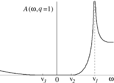
Figure 2: The electron spectral function in the reconstructed edge has singularities on the lines $\omega=v_{i}q$ that correspond to the edge excitation modes. The singularity at $\omega=v_{1}q$ is a divergence, and is the remnant of the $\delta$-peak in the unreconstructed edge. The spectral function vanishes for $v_{3}q<\omega<v_{2}q$ (e.g. for $q>0$) due to kinematic constrains. Shown is the case of the filling fraction $\nu=1/3$.

We now turn to the question of the possibility of experimental observation of the new features that appear in the electron spectral function as a result of edge reconstruction. It is clear that these features are associated with the redistribution of the weight of the original edge mode. Therefore, one should look for an experiment in which the observed quantity is most closely related to the spectral function itself and not its integral over $\omega$ or $q$. Such a situation is realized in the so-called momentum-resolved tunneling experiments. Kang ; Grayson In these experiments, the electron tunneling into the edge occurs across a barrier which is extended and homogeneous along the edge of the FQHE system, and so the electron’s momentum along the edge is conserved. In what follows, we consider the simplest possible case of tunneling from the (non-reconstructed) edge of the QHE at the filling fraction $\nu=1$ which is parallel to the reconstructed edge. The spectral function of the unreconstructed $\nu=1$ edge is just a $\delta$-function. This serves best to reveal the features of the spectral function of the reconstructed edge.

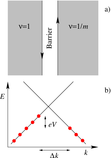
Figure 3: a) The setup consists of $\nu=1$ and reconstructed $\nu=1/m$ states separated by a barrier which is uniform along the edges; b) The structure of the energy dispersion in the vicinity of the barrier (see text for details).

The setup and the structure of energy levels under these conditions are shown in Fig. 3. The energy $E$ of the states is plotted as a function of momentum $k$ along the two parallel edges. The two straight lines in plot b) correspond to single electron dispersion on the two sides of the barrier. Near the intersection point of these lines, the states on the left and on the right begin to mix, and tunneling becomes possible. We shall treat tunneling using Fermi golden rule. Finally, we neglect the interaction between the edge modes on the opposite sides of the barrier, while the intra-edge interactions are taken into account by strong renormalization of the (charged) mode velocities.

In what follows, we shall consider separately two cases: $m=1$ and $m=3$. For energetic reasons, the edge of the QH state with higher $m$ is more susceptible to reconstruction, Wan-Yang-Rezayi however, the changes in the spectral function are more noticeable for lower $m$.

There are two parameters that one can control: bias voltage $V$ and magnetic field $B$. These two parameters are directly related to the structure of the spectrum: $eV$ sets the difference between the Fermi energies on the two sides of the barrier, while the difference between the two Fermi momenta $\Delta k\propto B-B_{0}$, where $B_{0}$ is the strength of the magnetic field at which, in the absence of bias, the Fermi energy lies exactly at the dispersion lines crossing point. Below, we shall rescale $B$ so that $\Delta k=B-B_{0}$.

Within our approximation, the tunneling current is given by the Fermi golden rule:

$$I(V,B) \propto \int A_{1}(\omega_{1},q_{1})A_{2}(\omega_{2},q_{2})[f(\omega_{1})-f(\omega_{2})]$$ (9)

$$\times\delta(eV+\omega_{1}-\omega_{2})\delta(B-B_{0}-q_{1}-q_{2})$$

$$\times d\omega_{1}d\omega_{2}dq_{1}dq_{2}.$$

Here, $A_{1}=\delta(\omega-v_{F}q)$ is the spectral function of the $\nu=1$ edge with the Fermi velocity $v_{F}$, and $A_{2}$ is the spectral function in Eq. (Electron Spectral Functions of Reconstructed Quantum Hall Edges); $f(\omega)$ is the Fermi distribution step function.

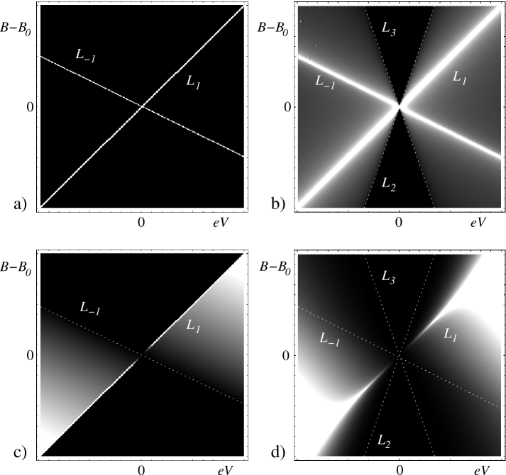
Figure 4: Differential conductance $dI/dV$ as a function of bias voltage $V$ and magnetic field $B$ for momentum-resolved tunneling from unreconstructed $\nu=1$ edge to: a) unreconstructed $\nu=1$ edge; b) reconstructed $\nu=1$ edge; c) unreconstructed $\nu=1/3$ edge; d) reconstructed $\nu=1/3$ edge. Plotted is the derivative of the result in Eq. (9). Parameters are: $v_{1}=1$, $v_{2,3}=\pm 1/3$, $v_{F}=2$, $\alpha_{1}=m=\nu^{-1}$, $\alpha_{2,3}=0.25$. The dashed lines are guides to the eye and are defined as $L_{1,2,3}=\{eV=v_{1,2,3}(B-B_{0})\}$, $L_{-1}=\{eV=-v_{F}(B-B_{0})\}$. See text for details.

The result of the numerical evaluation of the differential conductance $dI/dV$ as a function of $V$ and $B-B_{0}$ is shown in Fig. 4. In general, the plot of $dI(V,B)/dV$ is very similar, but not identical to $A_{2}(\omega,q)$. In particular, both have 3 lines of singularities (marked by letters $L_{1,2,3}$ on the figure), one of them being a divergence. These lines correspond to the three edge excitation modes $\omega=v_{i}q$. Moreover, in the bow-tie region between $L_{2}$ and $L_{3}$ the differential conductance (as well as the current itself) is exactly zero. The reason for this is purely kinematic: In the region below the dispersion line of the slowest excitation in the system, one cannot satisfy the conservation of energy and momentum in tunneling. This is best visible if one plots $dI/dV$ in a sweep of $V$ at fixed $B$. The resulting plot is very similar to that of the spectral function in Fig. 2. In the situation, where reconstruction produces multiple edges, this kinematic constraint dictates that $dI/dV=0$ in the region set by the two slowest velocities in the system.

We would like to point out, that while the singularities that correspond to the new neutral modes are rather weak and thus are difficult to observe, the general structure of the spectral weight transfer provides a clear indication of the edge reconstruction. In particular, in the bow-tie regions between $L_{1}$ and $L_{2}$, and between $L_{3}$ and $L_{-1}$, $dI/dV$ is zero before reconstruction and finite after. We note, that the rise of $dI/dV$ in the region between $L_{3}$ and $L_{-1}$ is due to the appearance of a (neutral) edge mode that propagates in the direction opposite to the direction of the original edge mode.

Although we have concentrated on the case of edge reconstruction described by a single point $k_{0}$, the preceding discussion remains generally valid for multiple edge reconstruction as well. In that case, new lines of singularities appear, while $L_{2}$ and $L_{3}$ correspond to the two slowest excitation modes.

A careful analysis Progress allows one to extract the precise form of the diverging singularities on $L_{1}$ and $L_{-1}$. The singularity on $L_{1}$ has the form: $[eV-v_{1}(B-B_{0})]^{\alpha_{2}+\alpha_{3}-1}$. The singularity on $L_{-1}$ has the form: $[eV+v_{F}(B-B_{0})]^{\alpha_{1}+\alpha_{2}+\alpha_{3}-2}$. In particular, the latter result explains why, given the Coulomb-interaction induced smallness of the exponents $\alpha_{2,3}$, the singularity on $L_{-1}$ in the $\nu=1/3$ case with $\alpha_{1}\approx 1/\nu=3$ (Fig. 4.d) is non-divergent. In principle, one should be able to extract independently the values of $\alpha_{1}$ and $\alpha_{2}+\alpha_{3}$ by fitting the experimental data to the above expressions, thus offering a consistency check, $\alpha_{1}\approx 1/\nu$, and a measure of the “strength” of reconstruction, $\alpha_{2}+\alpha_{3}$. Finally, the combination $\alpha_{1}+\alpha_{2}+\alpha_{3}$ is the exponent that describes the local tunneling into the reconstructed quantum Hall edge. Yang Momentum-resolved tunneling experiments thus offer an independent way of measuring this exponent.

Finally, we would like to comment on the role of the omitted $n\neq 0$ terms in Eq. (5). Apart from the factors $\exp ink_{0}x$, which trivially shift the momentum argument of the electron spectral function by $nk_{0}$, all terms with $n\neq 0$ are qualitatively similar to the $n=0$ term. Each of them produces a contribution to the Green’s function which is of the from Eq. (6), albeit with larger exponents $\alpha_{i}$. For that reason, all these terms make progressively less visible (but not necessarily unobservable) contributions to the spectral function.

Summarizing, we find that that edge reconstruction qualitatively changes the electron spectral function at the edge. The weight of the original sharp peak undergoes broad redistribution and the new edge modes that appear after the reconstruction show up as lines of singularities in the electron spectral function. We also suggest a momentum-resolved tunneling experiment which is best suited for probing the predicted features. We find that some of these features can be used to infer edge reconstruction.

We thank Matt Grayson, Woowon Kang and Leon Balents for helpful discussions. This work was supported by NSF grant No. DMR-0225698.

References

- (1) X.-G. Wen, Int. J. Mod. Phys. B 6, 1711 (1992).
- (2) A. H. MacDonald, S. R. E. Yang, and M. D. Johnson, Aus. J. Phys. 46, 345 (1993).
- (3) C. Chamon and X.-G. Wen, Phys. Rev. B 49, 8227 (1994).
- (4) X. Wan, K. Yang, and E. H. Rezayi, Phys. Rev. Lett. 88, 056802 (2002).
- (5) X. Wan, E. H. Rezayi, and K. Yang, Phys. Rev. B 68, 125307 (2003).
- (6) K. Yang, Phys. Rev. Lett. 91, 036802 (2003).
- (7) W. Kang, H. L. Stormer, L. N. Pfeiffer, K. W. Baldwin, and K. W. West, Nature 403, 59 (2000); I. Yang, W. Kang, K. W. Baldwin, L. N. Pfeiffer, and K. W. West, Phys. Rev. Lett. 92, 056802 (2004).
- (8) M. Huber, M. Grayson, D. Schuh, M. Bichler, W. Biberacher, W. Wegscheider, and G. Abstreiter, cond-mat/0309221; work in preparation.
- (9) U. Zülicke, E. Shimshoni, and M. Governale, Phys. Rev. B 65, 241315(R) (2002).
- (10) D. B. Chklovskii, B. I. Shklovskii, and L. I. Glazman, Phys. Rev. B. 46, 4026 (1992).
- (11) I. L. Aleiner and L. I. Glazman, Phys. Rev. Lett. 72, 2935 (1994).
- (12) O. G. Balev and P. Vasilopoulos, Phyr. Rev. Lett. 81, 1481 (1998).
- (13) O. Heinonen and S. Eggert, Phys. Rev. Lett. 77, 358 (1996).
- (14) D. Carpentier, C. Peça, and L. Balents, Phys. Rev. B 66 153304 (2002).
- (15) Kun Yang and A. Melikidze, unpublished.