Delays, Inaccuracies and Anticipation in Microscopic Traffic Models

Abstract

We generalize a wide class of time-continuous microscopic traffic models to include essential aspects of driver behaviour not captured by these models. Specifically, we consider (i) finite reaction times, (ii) estimation errors, (iii) looking several vehicles ahead (spatial anticipation), and (iv) temporal anticipation. The estimation errors are modelled as stochastic Wiener processes and lead to time-correlated fluctuations of the acceleration.

We show that the destabilizing effects of reaction times and estimation errors can essentially be compensated for by spatial and temporal anticipation, that is, the combination of stabilizing and destabilizing effects results in the same qualitative macroscopic dynamics as that of the respectively underlying simple car-following model. In many cases, this justifies the use of simplified, physics-oriented models with a few parameters only. Although the qualitative dynamics is unchanged, multi-anticipation increase both spatial and temporal scales of stop-and-go waves and other complex patterns of congested traffic in agreement with real traffic data. Remarkably, the anticipation allows accident-free smooth driving in complex traffic situations even if reaction times exceed typical time headways.

, url]http://www.mtreiber.de , url]http://www.akesting.de url]http://www.helbing.org

1 Introduction

The nature of human driving behaviour and the differences with the automated driving implemented in most micromodels is a controversial topic in traffic science [1, 2, 3, 4, 5, 6, 7, 8]. Finite reaction times and estimation capabilities impair the human driving performance and stability compared to automated driving, sometimes called ‘adaptive cruise control’ (ACC). However, unlike machines, human drivers routinely scan the traffic situation several vehicles ahead and anticipate future traffic situations leading, in turn, to an increased stability.

The question arises, how this behaviour affects the overall driving behaviour and performance, and whether the stabilizing effects (such as anticipation) or the destabilizing effects (like reaction times and estimation errors) dominate, or if they effectively cancel out each other. The answers to these questions are crucial for determining the influence of a growing number of vehicles equipped with automated acceleration control on the overall traffic flow. Up to now, there is not even clarity about the sign of the effect. Some investigations predict a positive effect [9], while others are more pessimistic [10].

Single aspects of human driving behaviour have been investigated in the past. For example, it is well known that traffic instabilities increase with the reaction times $T^{\prime}$ of the drivers. Finite reaction times in time-continuous models are implemented by evaluating the right-hand side of the equation for the acceleration (or velocity) at some previous time $t-T^{\prime}$ with $T^{\prime}>0$ [11, 12, 13]. Reaction times in time-continuous models have been modelled as early as 1961 by Newell [11]. Recently, the optimal-velocity model (OVM) [14] has been extended to include finite reaction times [12]. However, the Newell model has no dynamic velocity, and the OVM with delay turns out to be accident-free only for unrealistically small reaction times [15].

To overcome this deficiency, Davis [13] has introduced (among other modifications) an anticipation of the expected future gap to the front vehicle allowing accident-free driving at reaction times of 1 s. However, reaction times were not fully implemented in Ref. [13] since the own velocity, which is one of the stimuli on the right-hand side of the acceleration equation, has been taken at the actual rather than at the delayed time.

Another approach to model temporal anticipation consists in including the acceleration of the preceding vehicles in the input variables of the model. For cellular automata, this has been implemented by introducing a binary-valued ‘brake light’ variable [16].

To our knowledge, there exists no car-following model exhibiting platoon stability (with respect to all stimuli) for reaction times exceeding half of the time headway of the platoon vehicles. Human drivers, however, accomplish this task easily: In dense (not yet congested) traffic, the most probable time headways on German freeways are 0.9-1s [17, 18] which is of the same order as typical reaction times [19]. However, single-vehicle data for German freeways [17, 18] indicate that some drivers drive at headways as low as 0.3 s, which is below the reaction time of even a very attentive driver by a factor of at least 2-3 [19]. For principal reasons, therefore, safe driving is not possible in this case when considering only the immediate vehicle in front.

This suggests that human drivers achieve additional stability and safety by taking into account next-nearest neighbors and further vehicles ahead as well. Such ‘spatial anticipation’ or ‘multi-anticipation’ has been applied to the OVM [20] and to the Gipps model [21] as well as to some cellular automata model [16, 22]. As expected, the resulting models show a higher stability than the original model. However, the stability of the aforementioned models is still smaller than that of human driving. Furthermore, they display unrealistic behaviour such as clustering in pairs [21], or too elevated propagation velocities of perturbations in congested traffic ($v_{g}=-30$ km/h) [20].

Imperfect estimation capabilities often serve as motivation or justification to introduce stochastic terms into micromodels such as the Gipps model [23] (see also [2]). Most cellular automata require fluctuating terms as well. In nearly all the cases, fluctuations are assumed to be $\delta$-correlated in time and acting directly on the accelerations. An important feature of human estimation errors, however, is a certain persistency. If one underestimates, say, the distance at time $t$, the probability of underestimating it at the next time step (which typically is less than 1 s in the future) is high as well. Another source leading to temporally correlated acceleration noise lies in the concept of ‘action points’ modelling the tendency of human drivers to actively adapt to the traffic situation, i.e., to change the acceleration only at discrete times [24].

In this paper, we propose the human driver (meta-)model (HDM) in terms of four extensions to basic physics-oriented traffic models incorporating into these models (i) finite reaction times, (ii) estimation errors, (iii) spatial anticipation, and (iv) temporal anticipation. The class of suitable basic models is characterized by continuous acceleration functions depending on the velocity, the gap, and the relative velocity with respect to the preceding car and includes, for example, the optimal-velocity model (OVM) [14], the Gipps model [23], the velocity-difference model [25], the intelligent-driver model (IDM) [26], and the boundedly rational driver model [27, 28].

For matters of illustration, we will apply the HDM to the intelligent-driver model [26], which has a built-in anticipative and smooth braking strategy, and which reaches good scores in a first independent attempt to benchmark micromodels based on real traffic data [29].

In Sec. 2, we will formulate the HDM in terms of the acceleration function of the basic model. In Sec. 3 we will simulate the stability of vehicle platoons as a function of the reaction time $T^{\prime}$ and the number of anticipated vehicles $n_{a}$. We find string stability for arbitrarily long platoons for reaction times of up to 1.5 s. Furthermore, we simulate the macroscopic traffic dynamics for an open system containing a flow-conserving bottleneck [26, 30]. We find that multi-vehicle anticipation ($n_{a}>1$) can compensate for the destabilizing effects of reaction times and estimation errors. The numerically determined phase diagram for the corresponding parameter space gives the conditions under which simple physical models describe the traffic dynamics correctly. In the concluding Section 4, we suggest applications and further investigations and discuss some aspects of human driving that are not included in the HDM.

2 Modelling human driver behaviour

Let us formulate the HDM as a meta-model applicable to time-continuous micromodels (car-following models) of the general form

$$\frac{dv_{\alpha}}{dt}=a^{\rm mic}\left(s_{\alpha},v_{\alpha},\Delta v_{\alpha}\right),$$ (1)

where the own velocity $v_{\alpha}$, the net distance $s_{\alpha}$, and the velocity difference $\Delta v_{\alpha}$ to the leading vehicle serve as stimuli determining the acceleration $a^{\rm mic}$ [31]. This class of basic models is characterized by (i) instantaneous reaction, (ii) reaction only to the immediate predecessor, and (iii) infinitely exact estimating capabilities of drivers regarding the input stimuli $s$, $v$, and $\Delta v$, which also means that there are no fluctuations. In some sense, such models describe driving behaviour similar to adaptive cruise control systems.

For the sake of simplicity, we will restrict ourselves to single-lane longitudinal dynamics. Furthermore, we will not include adaptations of drivers to the traffic conditions of the last few minutes. This so-called ‘memory effect’ is discussed elsewhere [32].

2.1 Finite reaction time

A reaction time $T^{\prime}$ is implemented simply by evaluating the right-hand side of Eq. (1) at time $t-T^{\prime}$. If $T^{\prime}$ is not a multiple of the update time interval, we propose a linear interpolation according to

$$x(t-T^{\prime})=\beta x_{t-n-1}+(1-\beta)x_{t-n},$$ (2)

where $x$ denotes any quantity on the right-hand side of (1) such as $s_{\alpha}$, $v_{\alpha}$, or $\Delta v_{\alpha}$, and $x_{t-n}$ denotes this quantity taken $n$ time steps before the actual step. Here, $n$ is the integer part of $T^{\prime}/\Delta t$, and the weight factor of the linear interpolation is given by $\beta=T^{\prime}/\Delta t-n$. We emphasize that all input stimuli $s_{\alpha}$, $v_{\alpha}$, and $\Delta v_{\alpha}$ are evaluated at the delayed time.

Notice that the reaction time $T^{\prime}$ is sometimes set equal to the ‘safety’ time-headway $T$. It is, however, essential to distinguish between these times conceptually. While the time headway $T$ is a characteristic parameter of the driving style, the reaction time $T^{\prime}$ is essentially a physiological parameter and, consequently, at most weakly correlated with $T$. We point out that both the time headway $T$ and the reaction time $T^{\prime}$ are to be distinguished from the numerical update time step $\Delta t$, which is sometimes erroneously interpreted as a reaction time as well. For example, in our simulations, an update time step of 2 s has about the same effect as a reaction time of 1 s while the results are essentially identical for any update time step below 0.2 s.

2.2 Imperfect estimation capabilities

We will now model estimation errors for the net distance $s$ and the velocity difference $\Delta v$ to the preceding vehicle. Since the velocity itself can be obtained by looking at the speedometer, we neglect its estimation error. From empirical investigations (for an overview see [2], p. 190) it is known that the uncertainty of the estimation of $\Delta v$ is proportional to the distance, i.e., one can estimate the time-to collision (TTC) $s/|\Delta v|$ with a constant uncertainty [33]. For the distance itself, we specify the estimation error in a relative way by assuming a constant variation coefficient $V_{s}$ of the errors. Furthermore, in contrast to other stochastic micromodels [34], we take into account a finite persistence of estimation errors by modelling them as a Wiener process [35]. This leads to the following nonlinear stochastic processes for the distance and the velocity difference,

$$s^{\rm est}(t)=s(t)\,\exp(V_{s}w_{s}(t)),$$ (3)

$$(\Delta v)^{\rm est}(t)=\Delta v(t)+s(t)\,r_{\rm c}w_{\Delta v}(t),$$ (4)

where $V_{s}=\sigma_{s}/\mbox{$\langle s\rangle$}$ with $\sigma_{s}^{2}=\mbox{$\langle(s-\mbox{$\langle s\rangle$})^{2}\rangle$}$ is the variation coefficient of the distance estimate, and $1/r_{\rm c}$, a measure for the average estimation error of the time to collision. The stochastic variables $w_{s}(t)$ and $w_{\Delta v}(t)$ obey independent Wiener processes $w(t)$ of variance 1 with correlation times $\tau=1$ defined by [35]

$$\frac{dw}{dt}=-\frac{w}{\tau}+\sqrt{\frac{2}{\tau}}\,\xi(t),$$ (5)

with

$$\mbox{$\langle\xi\rangle$}=0,\ \ \mbox{$\langle\xi(t)\xi(t^{\prime})\rangle$}=\delta(t-t^{\prime}).$$ (6)

In the explicit numerical update from time step $t$ to step $t+\Delta t$, we implemented the Wiener processes by the approximations

$$w_{t+\Delta t}=e^{-\Delta t/\tau}w_{t}+\sqrt{\frac{2\Delta t}{\tau}}\eta_{t},$$ (7)

where the $\{\eta_{t}\}$ are independent realizations of a Gaussian distributed quantity with zero mean and unit variance. We have checked numerically that the update scheme (7) satisfies the fluctuation-dissipation theorem $\mbox{$\langle w_{t}^{2}\rangle$}=1$ for any update time interval satisfying $\Delta t\ll\tau$.

Simulations have shown that, in agreement with expectation, traffic becomes more unstable with increasing values of $V_{s}$ and $r_{c}$. To compare the influence of the temporally correlated multiplicative HDM noise with more conventional white acceleration noise, we have repeated the simulations of Section 3 with the deterministic HDM ($V_{s}=r_{c}=0$) augmented by an additive noise term $\sqrt{Q_{a}}\xi(t)$ at the right-hand side of the acceleration equation. Remarkably, the dynamics did not change essentially for reasonable values of the fluctuation strength $Q_{a}$. Thus, the more detailed representation of stochasticity by the HDM can be used to relate the conventional noise strength $Q$ (which does not have any intuitive meaning) to better justified noise sources.

2.3 Temporal anticipation

We will assume that drivers are aware of their finite reaction time and anticipate the traffic situation accordingly. Besides anticipating the future distance [13], we will anticipate the future velocity using a constant-acceleration heuristics. The combined effects of a finite reaction time, estimation errors and temporal anticipation leads to the following input variables for the underlying micromodel (1):

$$\frac{dv}{dt}=a^{\rm mic}(s^{\prime}_{\alpha},v^{\prime}_{\alpha},\Delta v^{\prime}_{\alpha})$$ (8)

with

$$s^{\prime}_{\alpha}(t)=\left[s_{\alpha}^{\rm est}-T^{\prime}\Delta v_{\alpha}^{\rm est}\right]_{t-T^{\prime}},$$ (9)

$$v^{\prime}_{\alpha}(t)=\left[v_{\alpha}^{\rm est}+T^{\prime}a_{\alpha}\right]_{t-T^{\prime}},$$ (10)

and

$$\Delta v^{\prime}_{\alpha}(t)=\Delta v_{\alpha}^{\rm est}(t-T^{\prime}).$$ (11)

We did not apply the constant-acceleration heuristics for the anticipation of the future velocity difference or the future distance, as the accelerations of other vehicles cannot be estimated reliably by human drivers. Instead, we have applied the simpler constant-velocity heuristics for these cases.

Notice that the anticipation terms discussed in this subsection (which do not contain any additional model parameters) are specifically designed to compensate for the reaction time by means of plausible heuristics. They are to be distinguished from ‘anticipation’ terms in some models aiming at collision-free driving in ‘worst-case’ scenarios (sudden braking of the preceding vehicle to a standstill) when the braking deceleration is limited. Such terms typically depend on the velocity difference and are included, e.g., in the Gipps model, in the IDM, and in some cellular automata [22, 36], but notably not in the OVM. The HDM is most effective when using a basic model with this kind of anticipation.

2.4 Spatial anticipation for several vehicles ahead

Let us now split up the acceleration of the underlying microscopic model into a single-vehicle acceleration on a nearly empty road depending on the considered vehicle $\alpha$ only, and a braking deceleration taking into account the vehicle-vehicle interaction with the preceding vehicle:

$$a^{\rm mic}(s_{\alpha},v_{\alpha},\Delta v_{\alpha}):=a^{\rm free}_{\alpha}+a^{\rm int}(s_{\alpha},v_{\alpha},\Delta v_{\alpha}).$$ (12)

Notice that this decomposition of the acceleration has already been used to formulate a lane-changing model for a wide class of micromodels [37].

Next, we model the reaction to several vehicles ahead just by summing up the corresponding vehicle-vehicle pair interactions $a^{\rm int}_{\alpha\beta}$ from vehicle $\beta$ to vehicle $\alpha$ for the $n_{\rm a}$ nearest preceding vehicles $\beta$:

$$\frac{d}{dt}v_{\alpha}(t)=a^{\rm free}_{\alpha}+\sum_{\beta=\alpha-n_{\rm a}}^{\alpha-1}a^{\rm int}_{\alpha\beta},$$ (13)

where all distances, velocities and velocity differences on the right-hand side are given by (9) - (11). Each pair interaction between vehicle $\alpha$ and vehicle $\beta$ is specified by

$$a^{\rm int}_{\alpha\beta}=a^{\rm int}\left(s_{\alpha\beta},v_{\alpha},v_{\alpha}-v_{\beta}\right),$$ (14)

where

$$s_{\alpha\beta}=\sum_{j=\beta+1}^{\alpha}\!\!s_{j}$$ (15)

is the sum of all net gaps between the vehicles $\alpha$ and $\beta$.

2.5 Applying the HDM extensions to the intelligent driver model (IDM)

In this paper, we will apply the HDM extensions to the IDM. In this model [26], the acceleration of each vehicle $\alpha$ is assumed to be a continuous function of the velocity $v_{\alpha}$, the net distance gap $s_{\alpha}$, and the velocity difference (approaching rate) $\Delta v_{\alpha}$ to the leading vehicle:

$$\dot{v}_{\alpha}=a\left[1-\left(\frac{v_{\alpha}}{v_{0}}\right)^{4}-\left(\frac{s^{*}(v_{\alpha},\Delta v_{\alpha})}{s_{\alpha}}\right)^{2}\right].$$ (16)

The IDM acceleration consists of a free acceleration $a^{\rm free}=a[1-(v/v_{0})^{4}]$ for approaching the desired velocity $v_{0}$ with an acceleration slightly below $a$, and the braking interaction $a^{\rm int}=-a(s^{*}/s)^{2}$, where the actual gap $s_{\alpha}$ is compared with the ‘desired minimum gap’

$$s^{*}(v,\Delta v)=s_{0}+vT+\frac{v\Delta v}{2\sqrt{ab}},$$ (17)

which is specified by the sum of the minimum distance $s_{0}$, the velocity-dependent safety distance $vT$ corresponding to the time headway $T$, and a dynamic part. The dynamic part implements an accident-free ‘intelligent’ braking strategy that, in nearly all situations, limits braking decelerations to the ‘comfortable deceleration’ $b$. Notice that all IDM parameters have an intuitive meaning. By an appropriate scaling of space and time, the number of parameters can be reduced from five to three.

Renormalisation for the intelligent driver model (IDM)

Remarkably, there exists a closed-form solution of the multi-anticipative IDM equilibrium distance as a function of the velocity,

$$s_{e}(v)=\gamma s^{*}(v,0)\left[1-\left(\frac{v}{v_{0}}\right)^{\delta}\right]^{-\frac{1}{2}},$$ (18)

which is $\gamma$ times the equilibrium distance of the original IDM [26], where

$$\gamma=\sqrt{\sum_{\alpha=1}^{n_{\rm a}}\frac{1}{\alpha^{2}}}.$$ (19)

The equilibrium distance $s_{e}(v)$ can be transformed to that of the original IDM by renormalizing the relevant IDM parameters appearing in $s^{*}(v,0)$:

$$s^{\rm ren}_{0}=\frac{s_{0}}{\gamma},\ \ T^{\rm ren}=\frac{T}{\gamma}.$$ (20)

The above renormalisation will be applied to all simulations of this paper. Notice that, in the limiting case of anticipation to arbitrarily many vehicles we obtain $\lim_{n_{\rm a}\to\infty}\gamma(n_{\rm a})=\pi/\sqrt{6}=1.283$. This means that the combined effects of all non-nearest-neighbor interactions would lead to an increase in the equilibrium distance by just about 28%.

Parameter	Value
Reaction time $T^{\prime}$	0 s - 2.0 s
Number of anticipated vehicles $n_{a}$	1 – 7
Relative distance error $V_{s}$	5%
Inverse TTC error $r_{c}$	0.01/s
Error correlation time $\tau$	20 s

Table 1: Parameters of the human-driver extensions with the values used in this paper. Unless stated otherwise, we have used the IDM parameters $v_{0}=128$ km/h, $T=1.1$ s, $a=1\ \mbox{m/s${}^{2}$}\$, $b=1.5\ \mbox{m/s${}^{2}$}\$, and $s_{0}=2$ m. In Section 3.1, we have changed $v_{0}$ and $T$ to 115 km/h and 1.5 s, respectively.

2.6 Summary of the human driver model (HDM)

The HDM is formulated in terms of a meta-model introducing reaction times, finite estimation capabilities, temporal anticipation and multi-vehicle anticipation to a wide class of simple micromodels. The model has two deterministic parameters, namely the reaction time $T^{\prime}$ and the number $n_{a}$ of anticipated vehicles whose influences will be investigated below.

The only stochastic contributions come from modeling finite estimation capabilities. The stochastic sources $V_{s}$ and $r_{c}$ characterize the degree of the estimation uncertainty of the drivers, while $\tau$ denotes the correlation time of errors. The limit $\tau\to 0$ corresponds to multiplicative white acceleration noise while $\tau\to\infty$ corresponds to ‘frozen’ error amplitudes, i.e., de facto heterogeneous traffic. All human-driver extensions are switched off and the original basic model is recovered if $T^{\prime}=0$, $n_{a}=1$, and $V_{s}=r_{c}=0$.

The HDM-IDM combination (i.e. the application of the HDM to the IDM) has a total number of ten parameters which can be reduced to eight by an appropriate scaling of space and time. Replacing the HDM noise by white additive noise (cf. Sec. 2.2) allows a further reduction to six parameters while retaining all essential properties.

3 Simulations and results

In this section, we apply the HDM extensions to the IDM for matters of illustration. In all simulations, we have used an explicit integration scheme assuming constant accelerations between each update time interval $\Delta t$ according to

$$\begin{array}[]{l}v_{\alpha}(t+\Delta t)=v_{\alpha}(t)+a_{\alpha}(t)\Delta t,\\ x_{\alpha}(t+\Delta t)=x_{\alpha}(t)+v_{\alpha}(t)\Delta t+\frac{1}{2}a_{\alpha}(t)(\Delta t)^{2}.\end{array}$$ (21)

Unless stated otherwise, we will use the IDM and HDM parameters given in Table 1. In the simulations, we will mainly study the influences of the reaction time $T^{\prime}$ and the number $n_{a}$ of anticipated vehicles.

3.1 String stability of a platoon

We have investigated the stability of the HDM as a function of the reaction time $T^{\prime}$ and the number $n_{a}$ of anticipated vehicles by simulating a platoon of $100$ vehicles following an externally controlled lead vehicle. As in a similar study for the OVM [15, 13], the lead vehicle drives at $v_{\rm lead}=15.34\>\mathrm{m/s}$ for the first 1000 s before it decelerates with $-0.7\>\mathrm{m/s}^{2}$ to $14.0\>\mathrm{m/s}$ and continues with this velocity until the simulation ends at $2500\>\mathrm{s}$.

For the platoon vehicles, we use the IDM parameters $v_{0}=32\>\mathrm{m/s}$ and $T=1.5\>\mathrm{s}$ to obtain the same desired velocity and initial equilibrium gap ($s_{\rm e}=25.7\>\mathrm{m}$) as in previous studies [15, 13]. The other IDM parameters are $a=1\,\mbox{m/s${}^{2}$}\$, $b=1.5\,\mbox{m/s${}^{2}$}\$, and $s_{0}=2$ m. If $n_{a}$ is larger than the number of preceding vehicles (which can happen for the first vehicles of the platoon) then $n_{a}$ is reduced accordingly. Fluctuations have been neglected in this scenario. As initial conditions, we have assumed the platoon to be in equilibrium, i.e., the initial velocities of all platoon vehicles were equal to $v_{\rm lead}$ and the gaps equal to $s_{e}$ so that the initial HDM (and IDM) accelerations were equal to zero.

We distinguish three stability regimes: (i) String stability, i.e., all perturbations introduced by the deceleration of the lead vehicles are damped away, (ii) an oscillatory regime, where perturbations increase but do not lead to crashes, and (iii) an instability with accidents. The condition for a simulation to be in the crash regime (iii) is fulfilled if there is some time $t$ and some vehicle $\alpha$ so that $s_{\alpha}(t)<0$. The condition for string stability is fulfilled if $|\dot{v}_{\alpha}(t)|<2\,\mbox{m/s${}^{2}$}\$ at all times (including the period where the leading vehicle decelerates) and for all vehicles, and additionally $|\dot{v}_{\alpha}(t)|<0.01\,\mbox{m/s${}^{2}$}\$ for all vehicles towards the end of the simulation. Finally, if neither the conditions for the crash regime nor that for the stable regime are fulfilled, the simulation result is attributed to the oscillatory regime.

Figure 1 shows the three stability regimes as a function of the reaction time $T^{\prime}$ and the platoon size $n$ for spatial anticipations of $n_{a}=1$ and $5$ vehicles, respectively. For $n_{a}=1$ (corresponding to conventional car-following models without spatial anticipation), a platoon of $100$ vehicles is stable for reaction times of up to $T^{\prime}_{\rm c1}=0.8\>\mathrm{s}$. Test runs with larger platoon sizes (up to 1000 vehicles) did not result in different thresholds suggesting that stability for a platoon size of 100 essentially means stability for arbitrarily large platoon sizes.

Increasing the spatial anticipation to $n_{a}=5$ vehicles shifted the threshold of the delay time $T^{\prime}$ for string stability of a platoon of 100 vehicles to $T^{\prime}_{\rm c1}=1.3\>\mathrm{s}$. Increasing the delay time $T^{\prime}$ beyond the stability threshold led to strong oscillations of the platoon. Crashes, however, occurred only when $T^{\prime}$ exceeded a second threshold $T^{\prime}_{\rm c2}$. Remarkably, for $n_{a}=5$ or more vehicles, the observed threshold $T^{\prime}_{\rm c2}=1.8\>\mathrm{s}$ is larger than the equilibrium time headway $s_{e}/v_{\rm lead}=1.68$ s. More detailed investigations reveal that crashes are triggered either directly by late reactions to deceleration maneuvers or indirectly as a consequence of the string instability. Further increasing $n_{a}$ do not change the thresholds significantly.

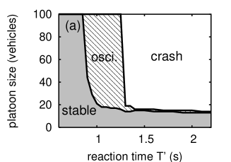
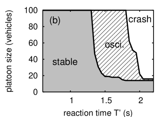
Figure 1: Stability of a platoon of identical vehicles as a function of the platoon size and the reaction time $T^{\prime}$ for the situation described in Section 3.1 (a) assuming conventional follow-the-leader behaviour ($n_{a}=1$) and (b) a reaction to $n_{a}=5$ vehicles. The simulation is for a time headway of $T=1.5\,\mathrm{s}$, a numerical update time interval of $\Delta t=0.1$ s, and a desired velocity $v_{0}=32\,\mathrm{m/s}$. The other parameters are given in Table 1. In the ‘stable’ phase, all perturbations are damped away. In the oscillatory regime, the perturbations increase, but do not lead to crashes.

3.2 Open system with a bottleneck

In this section we examine the opposite influences of the driver reaction time $T^{\prime}$ and the spatial anticipation $n_{a}$ on the stability of traffic and the occurring traffic states in a more complex and realistic situation.

We have simulated a single-lane road section of total length 20 km with a bottleneck and open boundaries assuming identical drivers and vehicles of length $l=5\>\mathrm{m}$, whose parameters are given in Table 1. The update time interval of the numerical integration was $\Delta t=0.1\>\mathrm{s}$. Each simulation run covered a time interval of $3\>\mathrm{h}$. We initialized the simulations with very light traffic of density 1 vehicle/km and set all initial velocities to 100 km/h.

We have simulated idealized rush-hour conditions by increasing the inflow $Q_{\rm in}(t)$ at the upstream boundary linearly from 100 veh/h at $t=0$ to 2100 veh/h at $t=1$ h, keeping the traffic demand constant afterwards. Since this demand exceeds the static road capacity $Q_{B}\approx 2000$ veh/h at the bottleneck (the maximum of the fundamental diagram), a traffic breakdown is always provoked, irrespective of the stability of traffic. We have implemented a flow-conserving bottleneck at 18 km $\leq x\leq$ 20 km by linearly increasing the IDM parameter $T$ from 1.1 s to 1.65 s in the region 18.0 km $\leq x\leq$ 18.5 km, setting $T=1.65$ s for 18.5 km $\leq x\leq$ 19.5 km, and linearly decreasing $T$ from 1.65 s to 1.1 s in the region 19.5 km $\leq x\leq$ 20.0 km (see Ref. [4] for a justification of this treatment of flow-conserving bottlenecks).

In order to determine the spatiotemporal dynamics, we plot, at any given spatiotemporal point $(x,t)$, the locally averaged velocity of the vehicle trajectories nearby. The averaging filter [38] had half-widths of 1 minute and 0.4 kilometers, respectively.

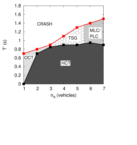
Figure 2: Phase diagram of congested traffic states in the phase space spanned by the number $n_{a}$ of anticipated vehicles and the reaction time $T^{\prime}$ in the open system with a bottleneck as described in the text. The dynamic phases HCT (homogeneous congested traffic), OCT (oscillatory congested traffic), TSG (triggered stop-and go), and MLC/PLC (moving and pinned localized clusters) are discussed in the main text.

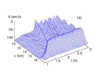
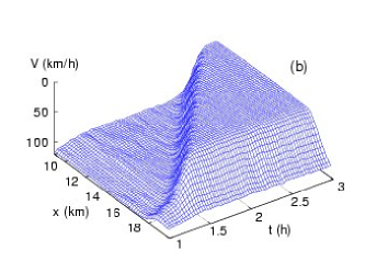
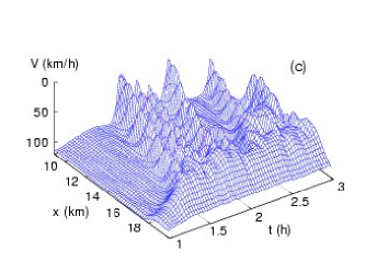
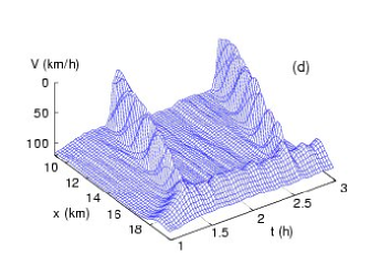
Figure 3: Spatiotemporal dynamics of typical traffic states of the phase diagram of Fig. 2. (a) The special case of the IDM ($n_{a}=1$, $T^{\prime}=0\>\mathrm{s}$) leads to oscillatory congested traffic (OCT); (b) $n_{a}=5$ anticipated vehicles and a reaction time $T^{\prime}=0.9\>\mathrm{s}$ leads to homogeneous congestion (HCT); even larger reaction times lead to (c) triggered stop-and-go traffic (TSG) ($n_{a}=5$, $T^{\prime}=1.1\>\mathrm{s}$) or (d) a combination of moving (MLC) and pinned localized clusters (PLC) ($n_{a}=6$, $T^{\prime}=1.2\>\mathrm{s}$). All data are smoothed with half-widths of 1 min and 0.4 km, respectively.

We have simulated the open system with $n_{a}=1$ to $n_{a}=7$. For each value of $n_{a}$, we have varied the reaction time in steps of 0.05 s. Figure 3 shows typical examples of the spatiotemporal patterns occuring in the simulations. By associating qualitatively different simulation results with different dynamical phases, we obtained a phase diagram in the space spanned by $n_{a}$ and $T^{\prime}$ (see Fig. 2). The different states were determined using smoothed velocity data, as shown in Fig. 3.

Specifically, a congested state may be either localized (localized cluster, LC) or extended (extended congested traffic, ECT). The criterion to discriminate between these two types of congested traffic is the width of the congested region which, for LCs, is constant (and typically less than 1 km), while the width of ECT is variable and depend in particular on the inflow. The transition between LC and ECT is slightly hysteretic. Furthermore, there are transitions from both LC and ECT to free traffic which are hysteretic as well.

Within ECT, there exist three dynamical phases separated by continuous phase transitions. As order parameter to distinguish between homogeneous congested traffic (HCT, cf. Fig. 3(b)) and oscillating congested traffic (OCT, cf. Fig. 3(a) and 4(c)) we have used the variance $\theta$ of the temporal velocity variations in the congested region sufficiently upstream of the bottleneck, where it is essentially constant with respect to space and time. While, in the case of HCT, $\theta$ depends mainly on the fluctuating forces and remains below 1 (m/s)², it jumps to more than 100 (m/s)² and essentially becomes independent of the fluctuation strength in the case of OCT. The third dynamical ECT phase are triggered stop-and go waves (TSG, cf. Fig. 3(c) and 4(b)). In contrast to OCT, TSG states reach the free branch of the fundamental diagram, i.e. there are uncongested areas between the congested ones. Nevertheless, the OCT and TSG states are hard to distinguish as they are not separated by a hysteretic phase transition.

Within localized clusters, we have observed a sharp transition between LCs moving upstream at a constant velocity of about $v_{g}=-15$ km/h (MLC), and clusters fixed at the bottleneck (PLC). In contrast to the IDM, we observed a coexistence of both localized dynamical phases (Fig. 3(d)), as required by observations [39].

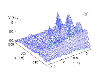
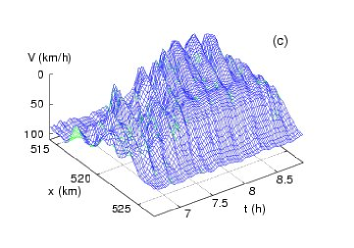
Figure 4: Spatiotemporal dynamics of congested traffic on the German freeway A9 South near Munich. (a) Sketch of the freeway. (b) Stop-and-go traffic (TSG) caused by the intersection I1 (cf. Fig. 3c). (c) Oscillatory congested traffic (OCT) caused by the intersection I2 (cf. Fig. 3a). The spatiotemporal data were obtained from one minute data at the detector positions indicated in (a), using the adaptive smoothing method [38] with smoothing half-widths of 1 min and 0.4 km, respectively.

Figure 5: Velocity time series by a virtual detector at $x=14$ km for (a) $n_{a}=1$, $T^{\prime}=0\>\mathrm{s}$, and (b) $n_{a}=5$, $T^{\prime}=1.1\>\mathrm{s}$. Notice the increase of the oscillation wavelength in the scenario (b) with anticipation.

Let us point out that our system is markedly different from the open system proposed by Kolomeisky et. al [40] where all phases are triggered by boundaries rather than by a bottleneck and which essentially contains only free traffic (FT) and the HCT state. Specifically, one can associate the ‘high-density’ state of [40] with HCT, while the ‘maximal-current’ state corresponds to the outflow region from HCT and finally the ‘low-density’ state corresponds to FT.

All of the above dynamic phases can be either reduced by varying the inflow and the bottleneck capacity [41, 42, 26], or by varying the model parameters, which we do in the following. The left lower corner of Fig. 2 corresponds to the special case of the IDM, i.e. to the case of zero reaction time ($T^{\prime}=0$) and consideration of the immediate front vehicle only ($n_{a}=1$). In this case, the simulation results in OCT for the boundary conditions specified before, see Figures 3(a), and 5(a).

Varying $n_{a}$ and $T^{\prime}$ leads to the following main results:

1. Traffic stability increases drastically, when the spatial anticipation is increased from $n_{a}=1$ to $6$, while the stability remains essentially unchanged for $n_{a}>6$.

2. For a sufficiently large number of anticipated vehicles, the congestion pattern becomes stable corresponding to homogeneous congested traffic (HCT) as shown in Fig. 3(b). Thus, different traffic states can be produced not only by varying the bottleneck strength as in the phase diagram proposed in Ref. [41], but also by varying model parameters that influence stability.

3. Increasing the reaction time $T^{\prime}$ destabilizes traffic and finally leads to crashes.

4. The other dynamic congested traffic states of the phase diagram presented in Ref. [41] are found as well, specifically, triggered stop-and-go waves (TSG), cf. Figures 3(c) and an interesting combination of moving localized clusters (MLC) and pinned localized clusters (PLC), see Fig. 3(d).

5. The results are robust against variations of the stochastic HDM parameters or when the correlated noise is replaced by white acceleration noise.

We have compared the spatiotemporal dynamics with traffic data from the German freeway A9 South near Munich. For this freeway, aggregated detector data (vehicle counts and average velocities for one-minute intervals) are available for each lane at the locations indicated in Fig. 4 (a). The plots (b) and (c) of Figure 4 show the spatiotemporal dynamics of the local velocity for triggered stop-and-go traffic (TSG) and oscillating congested traffic (OCT), respectively. In both cases, these states were caused by intersections acting as bottlenecks.

To obtain the spatiotemporal dynamics shown in these plots, we have applied the adaptive smoothing method (ASM) [38] to the lane-averages of the velocity data. The smoothing times and lengths of the ASM are set to the values used for the averaging filter in the simulation, i.e., to 1 min and 0.4 km, respectively. The other ASM parameters were set to $v_{c1}=30$ km/h, $v_{c2}=60$ km/h, $c_{\rm free}=80$ km/h, and $c_{\rm cong}=-15$ km/h [38]. We have checked that the result was essentially unchanged when changing any of the first three parameters by factors between 0.7 and 1.5. In contrast, changes of the last parameter $c_{\rm cong}$ representing the propagation velocity of collective structures in congested traffic influence the result. Artificial shifts of the congested structures are observed if $c_{\rm cong}$ is outside a range of about $[-17$ km/h, $-14$ km/h]. This means, besides making spatiotemporal plots, the ASM can be used to determine the propagation velocity $c_{\rm cong}$.

By comparing the simulation results 3(a) and (c) with the traffic data shown in 4(c) and (b), respectively, one sees a qualitative agreement of the spatiotemporal dynamics in many respects. Particularly,

1. the congestion pattern is triggered by a bottleneck,

2. the downstream front of the congestion pattern is stationary and located at the position of the bottleneck,

3. traffic is essentially non-oscillatory in a region of about 1 km width near the bottleneck (this is sometimes called the ‘pinch region’ [43]),

4. further upstream, the congested traffic consists of stop-and-go waves propagating upstream at a constant velocity $c_{\rm cong}$,

5. the period $\tau$ of the oscillations is variable.

Isolated and coexisting MLCs and PLCs as in Fig. 3(d) have been observed in traffic data as well [39]. Particularly, PLC and MLC states are shown in Fig. 6 and Fig. 10 of Ref. [39]. HCT states and even combined states of one or more PLCs with one or more isolated MLCs were also observed in [39].

In addition to these qualitative aspects, there exists a nearly quantitative agreement with respect to (i) the propagation velocity $c_{\rm cong}=-15$ km/h, and (ii) the range of the oscillation periods $\tau$ between 6 min and 40 min (notice that many car-following models yield too short periods). The latter point is illustrated by comparing Fig. 3(a) (no reaction time and no anticipation) and Fig. 3(c) (finite reaction time and anticipation) with the data, Fig. 4.

In summary, we have shown that the destabilizing effects of finite reaction times can be compensated to a large extent by spatial and temporal anticipation such that the resulting stability and dynamics are similar to the case of the IDM with zero anticipation and reaction time. However, besides stability issues, the HDM simulation results agree better with empirical traffic data in the following aspects: (i) Compared to the underlying IDM, the HDM simulation shows larger oscillation periods in the case of OCT and, generally, lower velocity gradients. (ii) Coexisting PLCs and MLCs are observed both in the HDM and in real traffic data [39], but not in the IDM. (iii) Near the bottleneck, the HDM regularly produces traffic of relatively high flow and density (’pinch region’).

4 Discussion

Finite reaction times and errors in estimating the input variables are clearly essential factors of driver behaviour affecting the performance and stability of vehicular traffic. However, these aspects are rarely considered in physics-oriented traffic modelling. Nevertheless, the simple models used by physicists such as the optimal-velocity model and its generalizations [14, 13], the velocity-difference model [25], or the IDM allow to describe many, particularly macroscopic, aspects of traffic dynamics such as the spatiotemporal dynamics of the various types of traffic congestion, the propagation of stop-and-go traffic, or even the scattering of flow-density data points of ‘synchronized traffic’ [4].

The question arises why, despite their obvious shortcomings, these models work so well. This question became more pressing after it turned out that all of the above models (including the IDM) produce unrealistic dynamics and crashes when simulating these models with realistic reaction times (of the order of 1 s).

In this work, we have shown that the destabilizing effects of reaction times and estimation errors can be compensated for by spatial and temporal anticipations: One obtains essentially the same longitudinal dynamics, which explains the good performance of the underlying simple models. In order to put this balance of stabilizing and destabilizing effects into a more general context, we have formulated the human-driver model (HDM) as a meta-model that can be used to extend a wide class of car-following models, where the acceleration depends only on the positions, velocities and accelerations of the own and the preceding vehicle. By applying the HDM extensions to the IDM, we have provided quantitative details of the balance conditions and the remaining differences in the dynamics. This involves validity criteria for the applicability of simpler physics-oriented car-following models.

Since the basic models have both the advantages and limitations of adaptive cruise control (ACC) systems, one can investigate the impact of ACC vehicles on the capacity and stability of the overall traffic simply by simulating a mixture of, e.g., IDM and HDM vehicles. Furthermore, one gets the nontrivial result that hypothetical future traffic consisting predominantly of automated vehicles will exhibit macroscopic dynamics similar to that of the actual traffic, although the driving strategy would be markedly different.

While finite reaction times have been investigated for more than 40 years [1] the HDM-IDM combination is, to our knowledge, the first car-following model allowing accident-free driving at realistic accelerations in all traffic situations for reaction times of the order of and even exceeding the time headway. A closer look at quantitative features of stop-and-go traffic or oscillations shows that, compared to simulations of the original IDM, the HDM extensions reduce the gradients of transitions between free and congested traffic and increase the wavelengths of stop-and-go waves, in agreement with empirical data. This suggests that multi-anticipation is an essential aspect of the driver behaviour.

A comparison of the stochastic HDM expressions for imperfect estimation capabilities with other stochastic micromodels is in order. While fluctuating terms were first introduced to traffic models more than 20 years ago [23], the most prominent example of stochastic traffic models are cellular automata (CA) of the Nagel-Schreckenberg type [34] and extensions thereof. There is, however, a qualitative difference compared with most continuous models: Fluctuation terms change the qualitative dynamics of many CA models. Therefore, they must be carefully chosen to yield plausible results. In contrast, the qualitative dynamics typically remains the same when fluctuations are added to car-following models via the HDM extensions. Having modelled the estimation errors by a stochastic Wiener process with a finite correlation time, we have included the persistence of estimation errors for a certain time interval.

The phase diagram shown in Fig. 2 contained qualitatively the same spatiotemporal congested states as found in Refs. [41, 26]. At first sight, this seems surprising. Besides using a different model, the control parameters making up the phase space were extrinsic in the previous work, while the phase space is spanned by intrinsic model parameters in the present work. A closer look at the analytic expressions for the phase boundaries [41] containing both extrinsic flow parameters and intrinsic stability limits indicates that variations of both kinds of control parameters can lead to phase transitions.

From a control-theoretical point of view, the HDM extensions implement a continuous response to delayed and noisy input stimuli. Alternatively, human driving behaviour can be modelled by so-called action-point models, where the response changes discontinuously whenever certain boundaries in the space spanned by the input stimuli are crossed [44, 24, 21], but these thresholds cannot easily confirmed by empirical data.

Finally, it should be mentioned that, in this work, we have considered only longitudinal aspects of human driving (acceleration and deceleration) and implemented only identical driver-vehicle units. Platooning effects due to different driving styles and the remarkable ability of human drivers to safely and smoothly change lanes even in congested conditions are the topic of a forthcoming paper.

Acknowledgments: The authors would like to thank for partial support by the DFG project He 2789/2-2 and the Volkswagen AG within the BMBF project INVENT.

References

- [1] D. Helbing, Traffic and related self-driven many-particle systems, Review of Modern Physics 73 (2001) 1067–1141.
- [2] M. Brackstone, M. McDonald, Car-following: a historical review, Transp. Res. F 2 (1999) 181–196.
- [3] E. Holland, A generalised stability criterion for motorway traffic, Transp. Res. B 32 (1998) 141–154.
- [4] D. Helbing, M. Treiber, Critical discussion of ”synchronized flow”, Cooper@tive Tr@nsport@tion Dyn@mics 1 (2002) 2.1–2.24, (Internet Journal, www.TrafficForum.org/journal).
- [5] K. Nagel, P. Wagner, R. Woesler, Still flowing: old and new approaches for traffic flow modeling, Operations Research 51 (2003) 681–710.
- [6] B. S. Kerner, The Physics of Traffic. Empirical Freeway Pattern Features, Engineering Applications, and Theory, Understanding Complex Systems, Springer, 2004.
- [7] D. Chowdhury, D. Santen, A. Schadschneider, Statistical physics of vehicular traffic and some related systems, Physics Reports 329 (2000) 199–329.
- [8] T. Nagatani, The physics of traffic jams, Reports of Progress in Physics 65 (2002) 1331–1386.
- [9] M. Treiber, D. Helbing, Microsimulations of freeway traffic including control measures, Automatisierungstechnik 49 (2001) 478–484.
- [10] G. Marsden, M. McDonald, M. Brackstone, Towards an understanding of adaptive cruise control, Transportation Research C 9 (2001) 33–51.
- [11] G. Newell, Nonlinear effects in the dynamics of car following, Operations Research 9 (1961) 209.
- [12] M. Bando, K. Hasebe, K. Nakanishi, A. Nakayama, Analysis of optimal velocity model with explicit delay, Phys. Rev. E 58 (1998) 5429.
- [13] L. Davis, Modifications of the optimal velocity traffic model to include delay due to driver reaction time, Physica A 319 (2002) 557.
- [14] M. Bando, K. Hasebe, A. Nakayama, A. Shibata, Y. Sugiyama, Dynamical model of traffic congestion and numerical simulation, Phys. Rev. E 51 (1995) 1035–1042.
- [15] L. Davis, Comment on ’analysis of optimal velocity model with explicit delay’, Phys. Rev. E 66 (2002) 038101.
- [16] W. Knospe, L. Santen, A. Schadschneider, M. Schreckenberg, Human behaviour as origin of traffic phases, Phys. Rev. E 65 (2001) 015101.
- [17] B. Tilch, D. Helbing, Evaluation of single vehicle data in dependence of the vehicle-type, lane, and site, in: D. Helbing, H. Herrmann, M. Schreckenberg, D. Wolf (Eds.), Traffic and Granular Flow ’99, Springer, Berlin, 2000, pp. 333–338.
- [18] W. Knospe, L. Santen, A. Schadschneider, M. Schreckenberg, Single-vehicle data of highway traffic: Microscopic description of traffic phases, Phys. Rev. E 65 (2002) 056133.
- [19] M. Green, ”How Long Does It Take to Stop?” Methodological analysis of driver perception-brake times, Transportation Human Factors 2 (2000) 195–216.
- [20] H. Lenz, C. Wagner, R. Sollacher, Multi-anticipative car-following model, European Physical Journal B7 (1998) 331–335.
- [21] N. Eissfeldt, P. Wagner, Effects of anticipatory driving in a traffic flow model, European Physical Journal B 33 (2003) 121–129.
- [22] H. K. Lee, R. Barlovic, M. Schreckenberg, D. Kim, Mechanical restriction versus human overreaction triggering congested traffic states, Physical Review Letters 92 (2004) 238702.
- [23] P. G. Gipps, A behavioural car-following model for computer simulation, Transp. Res. B 15 (1981) 105–111.
- [24] P. Wagner, I. Lubashevsky, Empirical basis for car-following theory development, cond-mat/0311192.
- [25] R. Jiang, Q. Wu, Z. Zhu, Full velocity difference model for a car-following theory, Phys. Rev. E 64 (2001) 017101.
- [26] M. Treiber, A. Hennecke, D. Helbing, Congested traffic states in empirical observations and microscopic simulations, Physical Review E 62 (2000) 1805–1824.
- [27] I. Lubashevsky, P. Wagner, R. Mahnke, Bounded rational driver models, European Physical Journal B 32 (2003) 243.
- [28] I. Lubashevsky, P. Wagner, R. Mahnke, Rational-driver approximation in car-following theory, Phys. Rev. E 68 (2003) 056109.
- [29] E. Brockfeld, R. Kühne, P. Wagner, Towards benchmarking microscopic traffic flow models, in: W. Möhlenbrink, M. Bargende, U. Hangleiter, U. Martin (Eds.), Networks for Mobility 2002, FOVUS: International Symposium, September 18-20, Stuttgart, Stuttgart, 2002, pp. 321–331.
- [30] M. Treiber, A. Hennecke, D. Helbing, Microscopic simulation of congested traffic, in: D. Helbing, H. Herrmann, M. Schreckenberg, D. Wolf (Eds.), Traffic and Granular Flow ’99, Springer, Berlin, 2000, pp. 365–376.
- [31] Inclusion of the acceleration of the preceding vehicle to the input variables is straightforward allowing for micromodels that model reactions to braking lights.
- [32] M. Treiber, D. Helbing, Memory effects in microscopic traffic models and wide scattering in flow-density data, Phys. Rev. E 68 (2003) 046119.
- [33] Generally, the estimation error concludes a systematic bias as well. We found that our model is very robust with respect to reasonable biases in distance and velocity-difference estimates.
- [34] K. Nagel, M. Schreckenberg, A cellular automaton modell for freeway traffic, J. Phys. I France 2 (1992) 2221–2229.
- [35] C. Gardiner, Handbook of Stochastic Methods, Springer, N.Y., 1990.
- [36] W. Knospe, L. Santen, A. Schandschneider, M. Schreckenberg, Disorder effects in cellular automata for two-lane traffic, Physica A 265 (1998) 614–633.
- [37] M. Treiber, D. Helbing, Realistische Mikrosimulation von Strassenverkehr mit einem einfachen Modell, in: D. Tavangarian, R. Grützner (Eds.), ASIM 2002, Tagungsband 16. Symposium Simulationstechnik, Rostock, 2002, pp. 514–520.
- [38] M. Treiber, D. Helbing, Reconstructing the spatio-temporal traffic dynamics from stationary detector data, Cooper@tive Tr@nsport@tion Dyn@mics 1 (2002) 3.1–3.24, (Internet Journal, www.TrafficForum.org/journal).
- [39] M. Schönhof, D. Helbing, Empirical Features of Congested Traffic States and their Implications for Traffic Modeling, cond-mat/0408138.
- [40] A. B. Kolomeisky, G. M. Schütz, E. B. K. J. P. Straley, Phase diagram of one-dimensional driven lattice gases with open boundaries, Journal of Physics A Mathematical General 31 (1998) 6911–6919.
- [41] D. Helbing, A. Hennecke, M. Treiber, Phase diagram of traffic states in the presence of inhomogeneities, Phys. Rev. Lett. 82 (1999) 4360–4363.
- [42] M. Treiber, A. Hennecke, D. Helbing, Derivation, properties, and simulation of a gas-kinetic-based, non-local traffic model, Phys. Rev. E 59 (1999) 239–253.
- [43] B. Kerner, Experimental features of self-organization in traffic flow, Phys. Rev. Lett. 81 (1998) 3797–3800.
- [44] R. Wiedemann, Simulation des Straßenverkehrsflusses, Schriftenreihe des IfV Vol. 8, Institut für Verkehrswesen, Universität Karlsruhe (1974).