The Vortex Kinetics of Conserved and Non-conserved O(n) Models

Abstract

We study the motion of vortices in the conserved and non-conserved phase-ordering models. We give an analytical method for computing the speed and position distribution functions for pairs of annihilating point vortices based on heuristic scaling arguments. In the non-conserved case this method produces a speed distribution function consistent with previous analytic results. As two special examples, we simulate the conserved and non-conserved $O(2)$ model in two dimensional space numerically. The numerical results for the non-conserved case are consistent with the theoretical predictions. The speed distribution of the vortices in the conserved case is measured for the first time. Our theory produces a distribution function with the correct large speed tail but does not accurately describe the numerical data at small speeds. The position distribution functions for both models are measured for the first time and we find good agreement with our analytic results. We are also able to extend this method to models with a scalar order parameter.

I Introduction

The phase ordering dynamics of certain physical systems after a rapid temperature quench below its critical temperature is dominated by the annihilation of topological defects of opposite charge [1]. In particular the $n$-vector model with non-conserved order parameter (NCOP) Langevin dynamics, where the defects are vortices, has been studied in some detail [2, 3, 4].

Mazenko [4, 5] carried out an investigation of the distribution of defect velocities for non-conserved phase ordering systems. By using an approximate “Gaussian closure” scheme, he was able to compute the velocity distribution for vortices in the non-conserved $n$-vector Langevin model for the case of point defects where $n=d$ dimensions. We [7] carried out numerical simulations for the $n=d=2$ non-conserved case and measured the vortices speed distribution. The results are consistent with Mazenko’s theoretical predictions. In particular the power-law tail of the distribution at large speeds which is robust is correctly predicted. The problem of the relative velocity as a function of separations for annihilating pairs was treated in Ref. [5], and the velocity distribution for strings for the non-conserved order parameter case was treated in Ref. [6].

Bray [8] developed a heuristic scaling treatment of the large speed tails based on the disappearance of small defects (annihilating pairs or contracting compact domains). This method treated only the power-law exponent of the distribution’s large speed tail. For the non-conserved $n$-vector case this simple argument gives a result consistent with Mazenko’s theory. However this method is also able to produce the large speed tail exponents for the conserved $n$-vector models, and conserved and non-conserved scalar (n=1) models.

We show here that Bray’s arguments can be extended to give results beyond the tail exponents. In models where point defects dominate the dynamics, one can compute the defect speed distribution functions based on Bray’s scaling assumption. The same idea can be easily generalized to the scalar order parameter case.

In a very recent work Mazenko [9] has suggested how the previous work in Ref. [4] can be extended to anisotropic systems and the conserved order parameter (COP) case. He finds that the average speed goes as $t^{-1}$ for the COP case with a scaling function of the same formal form as for the NCOP case given by Eq. (47) below. These results are not in agreement with the analytical or numerical work presented below in this paper. The Gaussian closure method developed in Ref. [9] does not appear adequate for treating the COP case.

In the next section we will generalize Bray’s argument for the point defect case. We find simple analytic expressions for the speed and separation distribution functions. We recover the large speed tail exponents obtained previously by Bray. For the non-conserved $n$-vector model we obtain precisely the same results as found in Ref. [4]. Then in Sec. III we present the numerical simulation results for non-conserved $n=d=2$ Langevin model. Next in Sec. IV, we present the simulations results for the conserved $n=d=2$ Langevin model. In Sec. V, we point out that the method developed in this paper can be used for those cases where one has a scalar order parameter.

II Theoretical Development

Let us suppose that we have $N$ pairs of oppositely charged vortices which are on their way to annihilation. We suppose that pair $i$ is separated by distance $r_{i}(t)$ with relative speed $v_{i}(t)=|\dot{r}_{i}(t)|$. Consider the associated phase-space distribution function:

$$f(r,v,t)=\langle\sum_{i=1}^{N}\delta(r-r_{i}(t))\delta(v-v_{i}(t))\rangle~{}~{}~{}.$$ (1)

This quantity satisfies the equation of motion

$$\frac{\partial}{\partial t}f(r,v,t)=-\frac{\partial}{\partial r}\langle\sum_{i=1}^{N}\dot{r}_{i}(t)\delta(r-r_{i}(t))\delta(v-v_{i}(t))\rangle-\frac{\partial}{\partial v}\langle\sum_{i=1}^{N}\dot{v}_{i}(t)\delta(r-r_{i}(t))\delta(v-v_{i}(t))\rangle~{}~{}~{}.$$ (2)

Our key kinematical assumption is that the relative velocity is a known function of the separation:

$$\dot{r}_{i}(t)=-v_{i}(t)=-u(r_{i}(t))$$ (3)

$$\dot{v}_{i}(t)=u^{\prime}(r_{i}(t))\dot{r}_{i}(t)=-u(r_{i}(t))u^{\prime}(r_{i}(t))~{}~{}~{}.$$ (4)

We check these assumptions as we proceed. Eq.(2) then takes the form

$$\frac{\partial}{\partial t}f(r,v,t)=\frac{\partial}{\partial r}\left(u(r)f(r,v,t)\right)+\frac{\partial}{\partial v}\left(u(r)u^{\prime}(r)f(r,v,t)\right)~{}~{}~{}.$$ (5)

where we have the normalization

$$\int_{0}^{\infty}dr\int_{0}^{\infty}dvf(r,v,t)=N(t)~{}~{}~{}.$$ (6)

Eq.(5) is one of our primary results.

Our assumptions are consistent with being in a regime where the annihilating pairs are independent and we can write

$$f(r,v,t)=N(t)P(r,v,t)$$ (7)

where $P(r,v,t)$ has the interpretation as the probability that at time $t$ we have a pair separated by a distance $r$ with relative speed $v$. Inserting Eq.(7) into Eq.(5) we find that $P(r,v,t)$ satisfies

$$\frac{\partial}{\partial t}P(r,v,t)=\frac{\partial}{\partial r}\left(u(r)P(r,v,t)\right)+\frac{\partial}{\partial v}\left(u(r)u^{\prime}(r)P(r,v,t)\right)+\gamma P(r,v,t)$$ (8)

where

$$\gamma=-\frac{1}{N(t)}\dot{N}(t)~{}~{}~{}.$$ (9)

We will see that $\gamma$ (and $N(t)$) are determined self-consistently by using scaling ideas.

We are interested in the reduced probability distributions

$$P_{r}(r,t)=\int_{0}^{\infty}dvP(r,v,t)~{}~{}~{},$$ (10)

and

$$P_{v}(v,t)=\int_{0}^{\infty}drP(r,v,t)$$ (11)

with the overall normalization

$$\int_{0}^{\infty}dr\int_{0}^{\infty}dvP(r,v,t)=1~{}~{}~{}.$$ (12)

Our goal is to solve Eq.(8). The first step is to show that

$$P(r,v,t)=P_{r}(r,t)\delta(v-u(r))~{}~{}~{}.$$ (13)

Inserting Eq.(13) into Eq.(8) we have

$$\delta(v-u(r))\frac{\partial}{\partial t}P_{r}(r,t)=\gamma\delta(v-u(r))P_{r}(r,t)+\frac{\partial}{\partial r}\left(u(r)\delta(v-u(r))P_{r}(r,t)\right)$$ (14)

$$+\frac{\partial}{\partial v}\left(u(r)u^{\prime}(r)\delta(v-u(r))P_{r}(r,t)\right)$$ (15)

$$=\delta(v-u(r))\left(\gamma P_{r}(r,t)+\frac{\partial}{\partial r}\left(u(r)P_{r}(r,t)\right)\right)$$ (16)

$$+u(r)P_{r}(r,t)\left(\frac{\partial}{\partial r}\delta(v-u(r))+\frac{\partial}{\partial v}u^{\prime}(r)\delta(v-u(r))\right)~{}~{}~{}.$$ (17)

Using the following identity

$$\frac{\partial}{\partial r}\delta(v-u(r))=\frac{\partial}{\partial r}\int\frac{d\lambda}{2\pi}e^{i\lambda(v-u(r))}$$ (18)

$$=\int\frac{d\lambda}{2\pi}(-i\lambda u^{\prime}(r)e^{i\lambda(v-u(r))}$$ (19)

$$=-u^{\prime}(r)\frac{\partial}{\partial v}\delta(v-u(r))$$ (20)

we find that Eq.(13) holds with $P_{r}(r,t)$ determined by

$$\frac{\partial}{\partial t}P_{r}(r,t)=\gamma P_{r}(r,t)+\frac{\partial}{\partial r}\left(u(r)P_{r}(r,t)\right)~{}~{}~{}.$$ (21)

Imposing the normalization,

$$\int_{0}^{\infty}drP_{r}(r,t)=1~{}~{}~{},$$ (22)

we find on integrating Eq. (21) over $r$ that

$$\gamma=\lim_{r\rightarrow 0}u(r)P_{r}(r,t)~{}~{}~{}.$$ (23)

Thus $\gamma$ and $N(t)$ are determined self-consistently in terms of the solution to Eq. (21).

So far this has been for general $u(r)$, let us restrict our subsequent work to the class of models where the relative velocity is a power law in the separation distance:

$$u=Ar^{-b}$$ (24)

where $A$ and $b$ are positive. Next we assume that we can find a scaling solution [11] to Eq. (21) of the form

$$P_{r}(r,t)=\frac{1}{L(t)}F(r/L(t))$$ (25)

where the growth law $L(t)$ is to be determined. Inserting this ansatz into Eq.(21) we obtain:

$$-L^{b}\dot{L}\left(xF^{\prime}+F\right)=Ax^{-b}F^{\prime}-Abx^{-b-1}F+L^{b+1}\gamma F$$ (26)

where $x=r/L(t)$. To achieve a scaling solution we require

$$L^{b}\dot{L}=AC$$ (27)

and

$$L^{b+1}\gamma(t)=AD$$ (28)

where $C$ and $D$ are time independent positive constants, the factors of $A$ are included for convenience. Eq. (26) then takes the form

$$-C\left[xF^{\prime}+F\right]=DF+x^{-b}F^{\prime}-bx^{-b-1}F~{}~{}~{}.$$ (29)

This has a solution

$$F(x)=\frac{Bx^{b}}{(1+Cx^{1+b})^{\sigma}}$$ (30)

where $B$ is an over all positive constant and the exponent in the denominator is given by

$$\sigma=1+\alpha/z$$ (31)

where $z=1+b$ and $\alpha=D/C$. If we enforce the normalization Eq. (22), we find that $D=B$. This reduces the spatial probability distribution to a function of two unknown parameters $B$ and $C$ assuming that $b$ is known.

We are at the stage where we can determine the number of annihilating vortex pairs as a function of time. From Eqs.(23), (9) and (30) we have that

$$\gamma(t)=\frac{AB}{L^{1+b}}=\frac{AD}{L^{1+b}}$$ (32)

and we again have that $D=B$. However from Eq.(27) we have

$$\frac{1}{1+b}\frac{d}{dt}L^{1+b}=AC$$ (33)

and for long times

$$L^{1+b}=ACzt~{}~{}~{}.$$ (34)

Putting this result back into Eq.(32) we find

$$\gamma(t)=\frac{AB}{ACzt}=\frac{\alpha}{zt}~{}~{}~{}.$$ (35)

We have then, from Eq. (9), that the number of pairs of vortices as a function of time is given by

$$N(t)/N(t_{0})=\left(t_{0}/t\right)^{\alpha/z}~{}~{}~{}.$$ (36)

However from simple scaling ideas we have rather generally that for a set of point defects in $d$ dimensions

$$N(t)\approx L^{-d}~{}~{}~{}.$$ (37)

Comparing this with Eq.(36) we identify $\alpha=d$. This gives our final form for $F(x)$

$$F(x)=\frac{Bx^{b}}{(1+Cx^{1+b})^{1+d/z}}~{}~{}~{}.$$ (38)

We check the validity of this result in sections III and IV.

The speed probability distribution is given by

$$P_{v}(v,t)=\int_{0}^{\infty}dr~{}P(r,v,t)$$ (39)

$$=\int_{0}^{\infty}dr~{}\delta(v-Ar^{-b})P_{r}(r,t)$$ (40)

$$=\frac{B}{AbL^{1+b}}\frac{1}{\tilde{v}^{2+1/b}}\left(1+\frac{C}{L^{1+b}\tilde{v}^{(1+b)/b}}\right)^{-\sigma}$$ (41)

where $\tilde{v}=v/A$. We can define the characteristic speed $\bar{v}$ via

$$\left(\frac{\bar{v}}{\tilde{v}}\right)^{(1+b)/b}=\frac{C}{L^{1+b}\tilde{v}^{(1+b)/b}}$$ (42)

or

$$\bar{v}(t)=\frac{C^{(1+b)/b}}{L^{b}}\propto t^{-(1-1/z)}$$ (43)

and

$$P_{v}(v,t)=\frac{B}{ACb\bar{v}}\frac{1}{V^{2+1/b}}\left(1+V^{-(1+b)/b}\right)^{-\sigma}=\frac{1}{\bar{v}}\,p_{v}(v/\bar{v})$$ (44)

where $V=\tilde{v}/\bar{v}$ and the distribution function has a scaling form. Clearly the large speed tail goes as $V^{-p}$ where $p=2+1/b$ in agreement with Bray’s result. After rearrangement we find

$$P_{v}(v,t)=\frac{1}{\bar{v}}\,p_{v}(v/\bar{v})=\frac{d}{Ab\bar{v}}\frac{V^{s}}{(1+V^{(1+b)/b})^{\sigma}}$$ (45)

where

$$s=\frac{B}{Cb}-1=\frac{d}{b}-1~{}~{}~{}.$$ (46)

We numerically test this result for various models below.

III Non-conserved n-vector model

We now want to test our theoretical results for $P_{r}(r,t)$ and $P_{v}(v,t)$ for the non-conserved time-dependent Ginzburg-Landau (TDGL) $O(n)$ model where $b=z-1=1$. If we work in terms of dimensionless variables ${\widetilde{v}}=v/\bar{v}$ and ${\widetilde{r}}=r/\bar{r}$ where $\bar{v}(t)$ and $\bar{r}(t)$ are the average speed and separation as function of time, then Eq. (45) gives the vortex speed distribution function

$$p_{v}({\widetilde{v}})=n\beta^{n/2}\frac{{\widetilde{v}}^{n-1}}{\left(1+\beta\,{\widetilde{v}}^{2}\right)^{(n+2)/2}}\ ,$$ (47)

with $\beta=\pi[\Gamma(\frac{1+n}{2})/\Gamma(\frac{n}{2})]^{2}$. This is exactly the familiar result found in Ref. [4] for $n=d$. The average speed is $\bar{v}\propto t^{-1/2}$ and $z=b+1=2$.

As a special case, when $n=2$, we have

$$p_{v}({\widetilde{v}})=\frac{2\beta{\widetilde{v}}}{\left(1+\beta\,{\widetilde{v}}^{2}\right)^{2}}\ ,$$ (48)

with $\beta=(\pi/2)^{2}=2.4674$. Both $p_{v}({\widetilde{v}})$ and $\bar{v}(t)$ have been verified in Ref. [7]. The energy and defect number are proportional to $(t/\ln t)^{-1}$, where there is a logarithmic correction. But we did not see such a correction for the average speed $\bar{v}(t)\propto t^{-1/2}$.

Let us turn next to the distance distribution function. From Eq. (38) we have, for $n=d=2$,

$$F({\widetilde{r}})=\frac{2C{\widetilde{r}}}{(1+C{\widetilde{r}}^{2})^{2}}\ ,$$ (49)

where $C=2.4674$.

We check this numerically using the same data as in Ref. [7]. The model is described by a Langevin equation defined in a two-dimensional space

$$\frac{\partial\vec{\psi}}{\partial t}=\epsilon\vec{\psi}+\nabla^{2}\vec{\psi}-(\vec{\psi})^{2}\vec{\psi}\ ,$$ (50)

where $\epsilon$ is set to be $0.1$, and the quench is to zero temperature, so we need not include noise. We worked on $1024\times 1024$ system with lattice spacing $\Delta r=\pi/4$. Periodic boundary conditions are used. Starting from a completely disordered state, we used the Euler method to drive the system to evolve in time with time step $\Delta t=0.02$.

The position of a vortex is given by the center of its core region, which is the set of points $(x_{i},y_{i})$ that satisfy $|\vec{\psi}(x_{i},y_{i})|<\langle|\vec{\psi}|\rangle/4$. By fitting $|\vec{\psi}(x_{i},y_{i})|$, where $(x_{i},y_{i})$ are the points belonging to a vortex’s core region, to the function $M(x,y)=A+B[(x-x_{0})^{2}+(y-y_{0})^{2}]$ we can find the center $(x_{0},y_{0})$. The positions of each vortex at different times are recorded, and the speed is calculated using $v=\Delta d/\Delta\tau$. Here $\Delta d$ is the distance that the vortex travels in time $\Delta\tau=5$.

To measure $\bar{r}(t)$ and $F({\widetilde{r}})$ we must first accumulate the following data. In a given run we keep track of the trajectories of all the vortex centers. We label each pair of oppositely charged vortices which annihilate. Then move backwards in time to determine for each such pair the separation as a function of time $r_{i}(t)$. Then $\bar{r}(t)$ is the average separation between annihilating pair of vortices at time $t$. The average distance $\bar{r}(t)$ is shown in Fig. 1. From the discussion in Sec. II we expect

$$\bar{r}(t)=L(t)=a\left[t+(\bar{r}_{0}/a)^{z}\right]^{1/z}\ ,$$ (51)

where $\bar{r}_{0}=\bar{r}(t=0)$ and $a$ is a constant. The average distance between annihilating pairs increases with time and a fit to the data gives $a=2.71$, $\bar{r}_{0}\approx 50$ and $z\sim 2.22$.

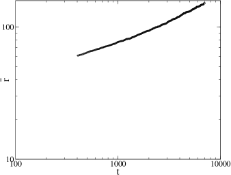
FIG. 1.: The average distance $\bar{r}$ between annihilating pairs versus time after quench. The data is averaged over 68 runs. The fit to the data is given by Eq. (51).

To measure the probability distribution function $F({\widetilde{r}})$, we distribute the various pairs into bins of width $\Delta=0.01$ centered about the scaled separation $r_{i}(t)/\bar{r}(t)$. We then plot the number of pairs in each bin versus $r(t)/\bar{r}(t)$ and properly normalize to obtain the scaling result shown in Fig. 2. In the following, when we measure the other distribution functions with scaling properties we employ the same method. The curve representing $F(x)$ given by Eq. (49) is also shown in Fig. 2. There is no free parameter in the fit other than $b$ and $\alpha$. The fit is fairly good. At large distances we can see the function approximately obeys a power law. The exponent is about $6$, which is different from the value 3 indicated by Eq. (49). We do not know why it is so.

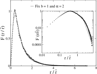
FIG. 2.: Separation probability distribution $F({\widetilde{r}})$ versus the scaled separation for the NCOP case with $n=d=2$. The data is averaged over 68 runs with a bin size of 0.01. The solid line is Eq. (49) with $b=1$ and $\alpha=2$. In the insert we show the same data on a logarithmic scale. At large $r$ the distribution is approximately a power law with an exponent about $6$. The dashed line in the insert is proportional to ${\widetilde{r}}^{-6}$.

We next measure $\bar{u}(r)$, the average speed for annihilating defects separating by a distance $r$. We track the motion of each annihilating pair, and determine for each pair the speed $u_{i}=(r_{i}(t+\Delta\tau)-r_{i}(t))/\Delta\tau$ as a function of $r_{i}$. Then we average $u_{i}(r)$ over all the pairs that have a fixed $r_{i}=r$. The result is shown in Fig. 3. For small enough separations we have $\bar{u}(r)\propto r^{-b}$ where $b\approx 1$ as expected.

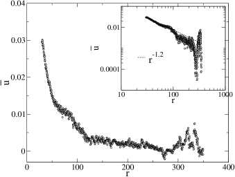
FIG. 3.: Test of Eq. (24). See text for a discussion. The data is averaged over 68 runs. There is a scaling regime at small distances $r$ with an exponent near to $-1$. At large distances, while the statistics are not as good, there is still an approximately power-law dependence on $r$.

IV Conserved n-vector model

Let us turn to the case of a conserved order parameter where for a TDGL model we expect $b=z-1=3$. In this case the vortex speed distribution, Eq. (45), is given by

$$p_{v}({\widetilde{v}})=\frac{n\beta^{n/4}}{3}\frac{{\widetilde{v}}^{(n-3)/3}}{\left(1+\beta\,{\widetilde{v}}^{4/3}\right)^{(n+4)/4}}$$ (52)

with $\beta=\left(n\Gamma(\frac{5}{4})\Gamma(\frac{3+n}{4})/\Gamma(1+\frac{n}{4})\right)^{4/3}$and the average speed is $\bar{v}\sim t^{-3/4}$. As a special case, consider $n=2$, where

$$p_{v}({\widetilde{v}})=\frac{2\sqrt{\beta}}{3}\,\frac{{\widetilde{v}}^{-1/3}}{\left(1+\beta\,{\widetilde{v}}^{4/3}\right)^{3/2}}\ ,$$ (53)

with $\beta=2.27773...$. Notice, unlike the NCOP case, $p_{v}({\widetilde{v}})$ blows up for small ${\widetilde{v}}$. This appears to be an unphysical feature.

The distribution function for the distance between annihilating pairs, Eq. (38) with $b=3$ and $n=d=2$, gives

$$F({\widetilde{r}})=\frac{2C{\widetilde{r}}^{3}}{(1+C{\widetilde{r}}^{4})^{3/2}}\ ,$$ (54)

where $C=11.817...$.

We simulated the conserved $O(2)$ model in two dimensions to test these predictions. The model is described by a Langevin equation defined on a two-dimensional space

$$\frac{\partial\vec{\psi}}{\partial t} = -\nabla^{2}\vec{\psi}-\nabla^{4}\vec{\psi}+\nabla^{2}\left[(\vec{\psi})^{2}\vec{\psi}\right]$$ (55)

$$= \nabla^{2}\frac{\delta{\mathcal{H}}_{E}[\vec{\psi}]}{\delta\vec{\psi}}\ ,$$ (56)

where the effective Hamiltonian is given by $\displaystyle{\mathcal{H}}_{E}[\vec{\psi}]=\int\left[-\frac{1}{2}\vec{\psi}^{2}+\frac{1}{2}(\nabla\vec{\psi})^{2}+\frac{1}{4}(\vec{\psi}^{2})^{2}\right]d^{2}r$. All the quantities are dimensionless. We work on $256\times 256$ system with lattice spacing $\Delta r=\pi/4$ and again periodic boundary conditions are used. We employ the method invented by Vollmayr-Lee and Rutenberg [10] to numerically integrate Eq. (55). This method is stable for any value of integration time step $\Delta t$. As the time $t$ increases, the evolution of the system becomes progressively slower. With the new time step technique we can increase the time step to accelerate the evolution. We let $\Delta t=0.01\,t^{0.36}$ after $t>120$.

In addition to the vortex statistics discussed in the NCOP case, we also measure the average energy $E=\langle{\mathcal{H}}_{E}\rangle$ above the ground state energy $E_{0}=-S/4$ with $S$ being the area of the system. The energy and number of vortices are shown in Fig. 4. The power-law exponent for the defect number is $-0.51$, which is consistent with $d/z=1/2$. The decay power law for the energy is $t^{-0.41}$, which is slower than that for the defect number. This may be due to the relaxation of spin waves.

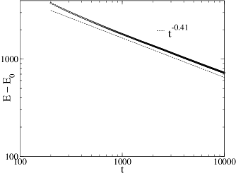
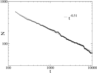
FIG. 4.: The energy $E(t)-E_{0}$ and the vortex number $N(t)$ are plotted versus time after quench. The data is averaged over 61 runs. The dashed lines, which are guides to the eye, are proportional to $t^{-0.41}$ for the energy plot and $t^{-0.51}$ for the vortex number plot respectively.

We use the same method as in the non-conserved case to find the center for each vortex. The speed of each vortex is computed by using $v=\Delta d/\Delta\tau$ with $\tau=10$. We measure the speed for each vortex at the same time $t$ and average over different vortices. The average speed of the defects is shown in Fig. 5. The prediction for the exponent is $-(1-1/z)=-0.75$, while the measurement finds $-0.77$.

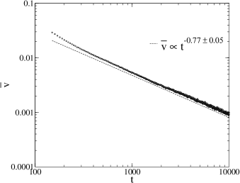
FIG. 5.: The averaged speed of vortices at time $t$ for the COP case. The data is averaged over 61 runs.

Next we determine the speed distribution as a function of time. Again we plot the scaled data from different times to test the scaling property of this distribution function. The resultant $p_{v}({\widetilde{v}})$ is shown in Fig. 6. Clearly scaling works and the large speed tail exponent is $2.24$. This is close to the prediction $2+1/b=2.33$. However the theory fails at small scaled speeds where the simulations go to zero while the theory blows up. Clearly the exponent $s$ in Eq. (38) is poorly determined in the theory for $b=2$ and $d=2$. If we allow $b$ and $\alpha$ float then we obtain an excellent fit shown in Fig. 6.

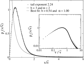
FIG. 6.: The probability distribution for vortex speed for the COP case. The data are from 61 different runs. The bin size is 0.01. The solid line is Eq. (53). The dashed line is the best fit to $p_{v}({\widetilde{v}})$ by changing $b$ and $\alpha$. In the insert we show the same data on a logarithmic scale. The dashed line in the insert is used to guide the eye and proportional to ${\widetilde{v}}^{-2.24}$.

The average separation of annihilating pairs of vortices $\bar{r}(t)$ for the COP case is shown in Fig. 7. Again fitting this to the form given by Eq. (51) we find $a=2.285$, $\bar{r}_{0}=17$ and $z=4.0$.

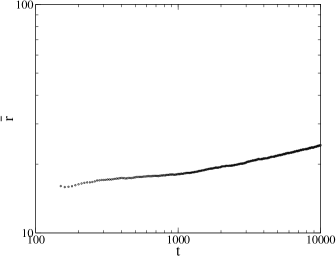
FIG. 7.: The average distance $\bar{r}$ between annihilating pair of vortices versus time after quench for the COP case. The data is from 61 runs. The fit to Eq. (51) is given in the text.

As in the NCOP case we can measure the separation distribution function $F({\widetilde{r}})$. This is shown in Fig. 8. With no free parameters, $b$ and $\alpha$ being fixed, the fit is pretty good. At large distances, the statistics are poor. But we can see the function approximately obeys a power law. The exponent is about $4$, which is different from the value 3 indicated by Eq. (54).

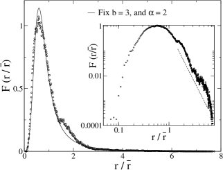
FIG. 8.: The probability distribution for the separation between two annihilating vortices for the COP case. The data is averaged over 61 runs. Bin size is 0.01. The solid line is Eq. (54) with $b=3$ and $\alpha=2$. In the insert we show the same data with a logarithmic scale. The behavior of this function at large distances is approximately a power law with an exponent about $4$. The dashed line is proportional to ${\widetilde{r}}^{-4}$.

We also measure $\bar{u}(r)$, as in the NCOP case. Our results are shown in Fig. 9. The assumption $u\sim r^{-b}$ is well satisfied with $b\approx 3$ at small enough distances.

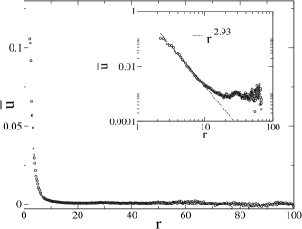
FIG. 9.: The average speed as a function of pair separation $r$ for the COP case. There is a scaling regime at small $r$ with the exponent near to $b=3$. The data is collected over 61 runs.

V Scalar models

We follow the argument given by Bray [8] to extend our discussion to include models with a scalar order parameter ($n=1$). First we calculate the probability function $P_{r}(r,t)$ for the domains with radius $r$. This calculation is the same with that in Sec. II. We obtain Eq. (33) for $F(x)$. Next, we compute the area-weighted probability for interfacial radius of curvature $r$ by multiplying $F(x)$ with $x^{d-1}$ and then normalize the resulting quantity. The resulting probability function $F_{s}(x)$ is

$$F_{s}(x)=\frac{d\Gamma(d/z)C^{(1+d+z)/z}}{\Gamma(1/2)\Gamma((d+z-1)/z)}\frac{x^{d+z-2}}{(1+Cx^{z})^{1+d/z}}\ .$$ (57)

Following Bray we use $v=Ar^{b}$ to get the distribution function for the interface speed

$$P_{v}({\widetilde{v}})=\frac{d\Gamma(d/z)\beta^{1/z}}{(z-1)\Gamma(1/z)\Gamma((d+z-1)/z)}\frac{{\widetilde{v}}^{-1+1/(z-1)}}{(1+\beta{\widetilde{v}}^{1+1/(z-1)})^{1+d/z}}\ .$$ (58)

For the non-conserved case, this result is the same with the one obtained by Bray using the Gaussian calculation. The large speed tail exponent is $p=2+d/(z-1)$, which is valid for both conserved and non-conserved models.

VI Conclusion

We show how a simple generalization of Bray’s scaling argument can lead to quantitative results for certain distribution functions. In particular we find that the distribution function for the distance between annihilating pairs of vortices is well described by the scaling theory for both NCOP and COP dynamics for $n=d=2$. We are also able to compute the speed distribution function using these ideas. For non-conserved models, we reproduce the accurate result obtained previously. For conserved models, the speed distribution function only gives us the correct tail exponent.

Our method can also be extended to scalar cases, and generate a full expression for the interfacial speed distribution. The power-law tail exponent $p=2+d/(z-1)$ is obtained. The result is the same as the result obtained by Bray [8].

The simple scaling method presented here leads to a reasonable description of the statistics of defect dynamics. Clearly it does a better job for the NCOP case since the speed distribution function for COP case does not show the proper small speed behavior. Similarly the more microscopic method of Ref. [9] leads to an adequate treatment of the small speed regime for the COP case but does not give the correct large speed tail.

The approach developed here is highly heuristic. Can it be systematized? Clearly to improve this approach one would need to include the interactions between different pairs. It is not clear how one does this.

Acknowledgement: This work was supported by the National Science Foundation under contract No. DMR-0099324 and by the Materials Research Science and Engineering Center through Grant No. NSF DMR-9808595.

REFERENCES

- [1] A. J. Bray, Adv. Phys. 43, 357 (1994).
- [2] F. Liu and G. F. Mazenko, Phys. Rev. B 46, 5963 (1992).
- [3] M. Mondello and N. Goldenfeld, Phys. Rev. A 42, 5865 (1990).
- [4] G. F. Mazenko, Phys. Rev. Lett. 78, 401 (1997).
- [5] G. F. Mazenko, Phys. Rev. E 56, 2757 (1997).
- [6] G. F. Mazenko, Phys. Rev. E 59, 1574 (1999). In this paper the speed distribution tail is given by where for non-conserved models ().
- [7] H. Qian and G. F. Mazenko, Phys. Rev. E 68, 021109 (2003).
- [8] A. J. Bray, Phys. Rev. E 55, 5297 (1997).
- [9] G. F. Mazenko, to be published, Phys. Rev. E (cond-mat/0308599).
- [10] B. P. Vollmayr-Lee and A. D. Rutenberg, Phys. Rev. E 68, 066703 (2003).
-
[11]
More generally Eq. (21) has the solution:
where and is an arbitrary function, and are two constants.(59)