Dynamics and phonon-induced decoherence of Andreev level qubit

Abstract

We present detailed theory for Andreev level qubit, the system consisting of a highly transmissive quantum point contact embedded in a superconducting loop. The two-level Hamiltonian for Andreev levels interacting with quantum phase fluctuations is derived by using the path integral method. We also derive kinetic equation describing qubit decoherence due to interaction of the Andreev levels with acoustic phonons. The collision terms are non-linear due to fermionic nature of the Andreev states, leading to slow non-exponential relaxation and dephasing of the qubit at temperature smaller than the qubit level spacing.

I Introduction

The possibility to employ Andreev bound levels in superconducting contacts for quantum computation has been suggested in Refs. [1, 2]. The proposed Andreev level qubit (ALQ) consists of a highly transmissive, with reflectivity $R\ll 1$, quantum point contact (QPC) embedded in a low inductance superconducting loop. In the ALQ, quantum information is stored in the microscopic two-level system of Andreev bound states in the contact. Hybridization of the clockwise and counterclockwise persistent current states in the ALQ loop is produced by the microscopic processes of electronic back scattering in the QPC. This is different from the macroscopic superconducting flux qubits[3, 4, 5] and charge-phase qubit[6], where the hybridization is provided by charge fluctuations on the tunnel junction capacitors. Thus requirement of the large charging energy or large loop inductance is not critical for the ALQ. A single ALQ consists of a pair of the Andreev bound levels belonging to the same normal conducting mode in the QPC; a multimode QPC will form a qubit cluster. The way of the ALQ operation is similar to the one of the experimentally tested flux qubits[3, 4, 5] - the Andreev levels can be excited by driving biasing magnetic flux through the qubit loop.[7, 8, 1] The read out method is also similar to the flux and charge-phase qubits: the quantum state of the Andreev levels determines the magnitude and direction of the persistent current circulating in the loop, and also the magnitude of the induced flux. Since the quantum information is stored in the microscopic system, Andreev levels, while the access for manipulation and readout is provided by macroscopic persistent currents, ALQ occupies an intermediate place between the microscopic solid state qubits (like localized spins on impurities[9] or quantum dots[10]) and macroscopic superconducting qubits.

During 90-s, the Josephson transport in superconducting QPCs has been intensively investigated, and a number of remarkable experiments has been performed on atomic size metallic QPCs using controllable break junction technique[11, 12], as well as on gated quantum constrictions in 2D electron gas confined between superconductors.[13] The critical Josephson current and current-voltage characteristics have been thoroughly examined in these experiments by applying current or voltage bias.[13, 14, 15, 16] There was, however, one experiment, particularly important in the qubit context, where the flux bias has been implemented: Koops et al.[17] have inserted metallic QPC in a SQUID, and evaluated the Josephson current-phase dependence by measuring the induced flux with an inductively coupled SQUID magnetometer. The measurements have been only reported for the equilibrium state. Unfortunately, no experimental attempts to drive the QPC out of equilibrium to some coherent or incoherent excited state have been performed so far.

The purpose of this paper is to present a theory for the Andreev level qubit in more detail than that was possible in short communication.[2] We will also consider the electron-phonon interaction as a potential ”intrinsic” source of the qubit decoherence, and derive a kinetic equation for the qubit density matrix. The ALQ Hamiltonian and the kinetic equation are derived by using a path integral method. [18, 19, 20] The central technical difficulty here is to extend the method to contacts with large transparency. This difficulty is overcome by incorporating exact boundary condition in the QPC action. Another important point discussed in the paper is the role of the charge electro-neutrality in the junction electrodes, which affects the qubit Hamiltonian.

The fermionic nature of the Andreev levels does not affect the qubit operation and qubit-qubit coupling but it plays important role for the qubit decoherence. We find that the electron-phonon collision terms in the kinetic equation for the ALQ differ qualitatively from the Bloch-Redfield master equation[21] commonly applied to study decoherence of the macroscopic superconducting qubits.[22] This results in long phonon-induced decoherence time for the ALQ, namely, at the temperature smaller than the qubit level spacing, both the relaxation and dephasing processes are governed by a power rather than exponential law.

The structure of the paper is the following. We discuss the model description of the QPC in Section II, and then explain in detail, in Section III, the path integral approach for transmissive QPC: we consider the action for the contact and derive the effective Hamiltonian for Andreev levels interacting with the quantum phase fluctuations; the single-particle density matrix, and effective current operator are also discussed in this section. In Section IV we discuss averaging over fast phase fluctuations and derive an effective Hamiltonian for the qubit, this procedure is extended in Section V to the two inductively coupled qubits to derive direct qubit-qubit interaction. Section VI is devoted to the electron-phonon interaction: we derive effective action for the Andreev level-phonon interaction and derive corresponding collision terms in the equation for the qubit density matrix; then we present solution of the kinetic equation, and evaluate the decoherence rate.

II Contact Hamiltonian

Let us consider a superconducting quantum point contact with bulk 3D electrodes. We model the contact with a smooth on the atomic scale (adiabatic) constriction and assume a local scatterer situated in the neck of constriction (see Fig. 1) producing weak electronic back scattering with the reflectivity $R\ll 1$. We further assume that the constriction supports a single conducting mode.

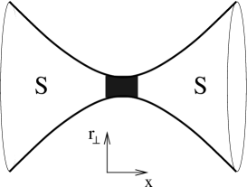
FIG. 1.: Adiabatic superconducting constriction with a local scatterer (dark region) in the neck. The length of the constriction is small on the scale of the superconducting coherence length but large on the atomic scale.

We adopt the mean field approximation for the electrons in the contact, which are described with the Hamiltonian,

$$H_{e}=\int d{\bf r}\;\Psi^{\dagger}({\bf r},t)h({\bf r},t)\Psi({\bf r},t)+{1\over 2}\,CV^{2}(t),$$ (1)

where the first term is the BCS Hamiltonian for the bulk superconducting electrons, $\Psi({\bf r},t)$ being the two-component Nambu field operator, and the second term describes the charging energy of the contact capacitor $C$ [18, 19, 20]. The single-particle Hamiltonian $h$ in Eq. (1) has the form,

$$h=\left[\,\frac{(-i\hbar{\bf\nabla}-(e/c){\bf A}({\bf r},t)\,\sigma_{z})^{2}}{2m}-\mu+U({\bf r})+e\varphi({\bf r},t)\,\right]\sigma_{z}+\Delta({\bf r},t)\,e^{i\sigma_{z}\chi({\bf r},t)}\sigma_{x}\,,$$ (2)

where $\Delta({\bf r},t)$ and $\chi({\bf r},t)$ are, respectively, the modulus and phase of the superconducting order parameter, the potential $U({\bf r})$ accounts for the confinement of electrons within the contact as well as the electron scattering, while $\varphi({\bf r},t)$ and ${\bf A}({\bf r},t)$ are electromagnetic potentials. The voltage drop at the contact, $V(t)$, in Eq. (1) is related to the discontinuity of the electric potential at the contact, $V(t)=\varphi(-0,t)-\varphi(+0,t)$. To investigate the decoherence effects, we allow the electrons in the electrodes to interact with acoustic phonons, and include corresponding electron-phonon interaction and phonon terms in the total Hamiltonian of the contact,

$$H_{c}=H_{e}+H_{e-ph}+H_{ph}\,.$$ (3)

It is convenient to introduce quasiclassical (Andreev) approximation for the superconducting electrons. Following standard procedure, we eliminate rapidly varying in space potential, $U({\bf r})$, by introducing quasiclassical wave functions of the single conducting mode in the left and right electrodes,

$$\Psi({\bf r},t)=\sum_{\sigma=\pm}\psi_{\perp}({\bf r}_{\perp},x)\,e^{i\sigma\int dx\,k(x)}\,\psi^{(\sigma)}(x,t)\,,$$ (4)

and couple these wave functions by means of a normal electron scattering matrix. In Eq. (4), $\psi^{(\sigma)}(x)$ are slowly varying 1D envelopes for the longitudinal electron motion ($\sigma=\pm$ indicates the direction of the motion), $\psi_{\perp}({\bf r}_{\perp},x)$ is a normalized wave function of the transverse motion with energy $E_{\perp}(x)$, $p(x)=\hbar k(x)=\sqrt{2m\left(\mu-E_{\perp}(x)\right)}=mv(x)$ is the quasiclassical longitudinal electronic momentum. The coupling of the quasiclassical envelopes in the left ($L$) and right ($R$) electrodes, $\psi_{L,R}$, is conveniently described by the transfer matrix, [7, 23]

$$\left(\begin{array}[]{c}\psi^{(+)}_{L}\\ \psi^{(-)}_{L}\end{array}\right)(0,t)=\hat{T}\left(\begin{array}[]{c}\psi^{(+)}_{R}\\ \psi^{(-)}_{R}\end{array}\right)(0,t)\;,$$ (5)

$$\hat{T}=\left(\begin{array}[]{cc}1/d&r^{\ast}/d^{\ast}\\ r/d&1/d^{\ast}\end{array}\right)\,.$$ (6)

Here $d$ and $r$ are the energy independent transmission and reflection amplitudes, respectively. Since any observable quantity is expressed through a bilinear combination of the envelopes with the same $\sigma$, the energy independent scattering phases can be eliminated from the boundary condition (5), hence, without loss of generality, the scattering amplitudes will be further assumed to be real, $d=\sqrt{D}$, $r=\sqrt{R}$, where $D$ and $R$ are the transmission and reflection coefficients of the contact, respectively.

The electromagnetic potentials, $\varphi({\bf r},t)$, ${\bf A}({\bf r},t)$, and the complex order parameter in Eq. (2) are to be found from the Maxwell equations and the self-consistency equation. It is convenient to present the Hamiltonian in a gauge invariant form by extracting the phase of the order parameter using a local gauge transformation, $\Psi({\bf r},t)\rightarrow e^{i\sigma_{z}\chi({\bf r},t)/2}\,\Psi({\bf r},t)\,.$ Then the superfluid momentum ${\bf p}_{s}=\hbar{\nabla}\chi/2-(e/c){\bf A}$, and the gauge-invariant electric potential $\tilde{\varphi}=\hbar\dot{\chi}/2+e\varphi$, appear in the quasiclassical Hamiltonian of the electrode,

$$h^{(\sigma)}=\sigma v(-i\hbar\partial_{x})\,\sigma_{z}+\sigma vp_{s}+\tilde{\varphi}\,\sigma_{z}+\Delta\,\sigma_{x},$$ (7)

while the phase difference $\phi(t)=\chi_{R}(0,t)-\chi_{L}(0,t)$, appears in the boundary condition,

$$\hat{T}\rightarrow e^{i\sigma_{z}\phi(t)/2}\;\hat{T}\,.$$ (8)

In the bulk metallic electrodes with good screening, and at small frequencies relevant for the problem, the gauge-invariant fields, $\tilde{\varphi}({\bf r},t)$, ${\bf p}_{s}({\bf r},t)$, are to be found from the electro-neutrality condition, and the current conservation,[24, 25, 26]

$$\delta n({\bf r},t)=0,\;\;\;\nabla{\bf j}({\bf r},t)=0,$$ (9)

where $n({\bf r},t)$ is the electronic density. In the electrodes, the charge imbalance relaxation yields the equilibrium relation, $\tilde{\varphi}=(\partial n/\partial\mu)^{-1}\delta n$, on the distance exceeding the electric field penetration length. Furthermore, in the absence of normal dissipative current, ${\bf p}_{s}$ is proportional to the total current density, ${\bf j}=(en/m){\bf p}_{s}$, which is negligibly small far from the contact due to rapid spreading out of the current in the point contact geometry. Thus the conditions (9) yield complete cancellation of the electromagnetic potentials in the electrodes,

$$\tilde{\varphi}(x,t)=0,\;\;\;p_{s}(x,t)=0\,.$$ (10)

Taking into account that the modulus of the order parameter far from the contact is equal to the equilibrium value,[27] $\Delta={\rm const}$, we conclude that the Hamiltonian (7) approaches the equilibrium form.

Potential $\tilde{\varphi}$ can be expressed through the electric field $E$, $\tilde{\varphi}=\hbar\dot{\bar{\chi}}/2+e\int dx\,E$, by introducing the gauge invariant phase $\bar{\chi}=\chi-(2e/c\hbar)\int dx\,A=(2/\hbar)\int dx\,p_{s}$. The spatial distribution of these quantities is illustrated on Fig. 2. Since $\tilde{\varphi}$ vanishes far from the contact, and $\bar{\chi}$ is constant according to Eq. (10), then the gauge-invariant phase difference across the contact $\dot{\bar{\phi}}=\dot{\bar{\chi}}_{R}(0,t)-\dot{\bar{\chi}}_{L}(0,t)$ is related to the voltage drop, $V=\int_{-\infty}^{\infty}dx\,E$ ,

$$\dot{\bar{\phi}}(t)={2eV\over\hbar}$$ (11)

(Josephson relation). In the SQUID, this relation is equivalent to the phase versus flux relation, $\bar{\phi}=2e\Phi/\hbar c$, since the voltage drop across the contact is generated by time variation of the magnetic flux $\Phi$ threading the SQUID. Finally, we notice that the gauge-invariant phase difference, $\bar{\phi}$, rather than $\phi$ enters the boundary condition (8), which can be explicitly seen by extracting the Aharonov-Bohm phase from the transfer matrix. Thus the gauge-invariant phase difference remains the only free collective variable whose dynamics is determined by the electrodynamic environment of the contact. Below we will not distinguish between $\bar{\phi}$ and $\phi$, because the difference is negligibly small in the QPC.

FIG. 2.: Spatial distribution of the electric potential, $\varphi$ (thin line), gauge invariant potential, $\tilde{\varphi}$ (bold line), and the time derivative of the gauge invariant phase, $\dot{\bar{\chi}}$ (dashed line), in the vicinity of the contact.

Proceeding with discussion of the interaction of electrons with phonons, we consider only longitudinal acoustic phonons and describe the interaction within the deformation potential approximation,

$$H_{e-ph}=\gamma\int d{\bf r}\,\nabla{\bf u}({\bf r},t)\,\Psi^{\dagger}({\bf r},t)\sigma_{z}\Psi({\bf r},t),$$ (12)

where $\gamma$ is the deformation potential constant, ${\bf u}({\bf r},t)$ is the phonon field operator,

$${\bf u}({\bf r})=\sum_{\bf q}\sqrt{{\hbar\over 2\rho V\Omega_{q}}}\,{{\bf q}\over q}\,\left(b_{\bf q}\,e^{i{\bf qr}}+b^{\dagger}_{\bf q}\,e^{-i{\bf qr}}\right)\;,\;\;\;\Omega_{q}=sq\,,$$ (13)

$s$ is the sound velocity, and $\rho$ is the crystal mass density. The Hamiltonian of free phonons has a standard form,

$$H_{ph}=\sum_{\bf q}\hbar\Omega_{q}\left(b^{\dagger}_{\bf q}b_{\bf q}+1/2\right).$$ (14)

Our strategy now will be to derive effective Hamiltonian for the Andreev levels including interaction with phonons. If the phase difference would be a classical variable, this derivation can be in principle done by direct truncation of the Hamiltonian (3). However, in the presence of quantum phase fluctuations it is convenient to apply the path integral technique.

III Contact effective action

Let us consider the whole system, the QPC and superconducting loop (see Fig. 3), and introduce the path integral representation for the propagator,

$${\cal U}=\int{\cal D}^{2}\psi_{L}{\cal D}^{2}\psi_{R}\,{\cal D}\{X_{\bf q}\}\,{\cal D}\phi\,e^{i\int dtL_{tot}/\hbar}\;,\;\;\;X_{\bf q}=b_{\bf q}+b_{\bf q}^{\ast}\,.$$ (15)

The Lagrangian of the system $L_{tot}$ consists of the contact part $L_{c}$, and the part describing the circulating current in the loop. The latter is conveniently combined with the charge term from the electronic Hamiltonian (1) giving the Lagrangian of the loop oscillator $L_{osc}$,

$$L_{tot}=L_{c}+L_{osc},\;\;L_{osc}=\left({\hbar\over 2e}\right)^{2}\left({C\over 2}\,(\partial_{t}\phi)^{2}-{c^{2}\over 2L}\,(\phi-\phi_{e})^{2}\right)\,,$$ (16)

where $\phi_{e}$ corresponds to the bias magnetic flux, and $L$ is the loop inductance. The remaining part of the contact Lagrangian consists, similar to Eq. (3), of the electronic part, phonon part, and electron-phonon interaction,

$$L_{c}=L_{e}+L_{ph}+L_{e-ph}\,.$$ (17)

In the quasiclassical approximation, the electronic Lagrangian splits into two parts, $L_{\alpha}$, $\alpha=L,R$, corresponding to the left and right electrodes,

$$L_{\alpha}=\sum_{\sigma=\pm}\int dx\,\bar{\psi}_{\alpha}^{(\sigma)}(x,t)\,{\cal L}^{(\sigma)}(x,t)\,\psi_{\alpha}^{(\sigma)}(x,t)\,,\;\;{\cal L}^{(\sigma)}(x,t)=i\hbar\partial_{t}+\sigma vi\hbar\partial_{x}\sigma_{z}-\Delta\sigma_{x}\,,$$ (18)

and the third part $L_{BC}$ discussed in detailed in the next section, which accounts for the boundary condition. Noting that relaxation processes are caused by phonons with small wave vectors compared to the Fermi wave vector, $q\ll k$, transitions between the states $\psi^{(+)}$ and $\psi^{(-)}$ are forbidden, and the electron-phonon Lagrangian can be written on the form,

$$L_{e-ph}=-\gamma\sum_{\alpha=L,R}\sum_{\sigma=\pm}\int d{\bf r}\;|\psi_{\perp}|^{2}\,\bar{\psi}_{\alpha}^{(\sigma)}(x,t)\,\sigma_{z}\,\psi_{\alpha}^{(\sigma)}(x,t)\nabla{\bf u}({\bf r},t)\,.$$ (19)

The phonon Lagrangian is given by equation,

$$L_{ph}={1\over 2}\sum_{\bf q}\,(\hbar/2\Omega_{q})\,X_{\bf q}\left[(i\partial_{t})^{2}-\Omega_{q}^{2}\right]X_{\bf q}\,.$$ (20)

FIG. 3.: Sketch of the Andreev level qubit: a low inductance superconducting loop with a quantum point contact (QPC). $\Phi$ is the magnetic flux; the arrows indicate fluctuating persistent currents.

A Boundary condition

The boundary condition (5) is valid for any contact transparency. To include this boundary condition in the path integral formulation, we introduce an additional term in the Lagrangian[2],

$$L_{BC}=\bar{\eta}(t)\sum_{\sigma}\left[\sqrt{D}\,e^{-i\sigma_{z}\phi(t)/4}\psi_{L}^{(\sigma)}(0,t)-(1+\sqrt{R})e^{i\sigma_{z}\phi(t)/4}\psi_{R}^{(\sigma)}(0,t)\right]+h.c.\,,$$ (21)

where $\eta$ is an auxiliary fermionic Nambu field playing the role of a Lagrange multiplier. Correspondingly, the integration over $\eta$ is to be included in the propagator in Eq. (15), giving the following form for the electronic part of the propagator,

$${\cal U}_{e}=\int{\cal D}^{2}\eta\,{\cal D}^{2}\psi_{L}{\cal D}^{2}\psi_{R}\,e^{i\int dt(L_{L}+L_{R}+L_{BC})/\hbar}\,.$$ (22)

Let us prove that such a Lagrangian indeed generates the boundary condition (5), (8). To this end, it is convenient to make a step back and restore a non-quasiclassical form for the fermionic field,

$$\psi(x,t)=\sum_{\sigma}e^{i\sigma\int kdx}\,\psi^{(\sigma)}(x,t)\,,$$ (23)

in the bulk part of the Lagrangian,

$$L_{L}\,+\,L_{R}=\int_{-\infty}^{\infty}dx\,\bar{\psi}(x,t){\cal L}(x,t)\psi(x,t),\;\;\;{\cal L}(x,t)=i\hbar\partial_{t}-[(-\hbar^{2}/2m)\partial_{x}^{2}+E_{\perp}-\mu]\,\sigma_{z}-\Delta\,\sigma_{x}\,.$$ (24)

The dynamic equations and the boundary condition result from the zero variation of the action $S_{e}=\int dt\,(L_{L}+L_{R}+L_{BC})$ with respect to $\bar{\psi}_{L,R}$ and $\bar{\eta}$,

$${\delta S_{e}\over\delta\bar{\psi}_{L,R}(x,t)}=0\;,\;\;\;{\delta S_{e}\over\delta\bar{\eta}(t)}=0\,,$$ (25)

or in the explicit form,

$${{\cal L}}(x,t)\,\psi_{L}(x,t) = -\sqrt{D}\,\delta(x)\,e^{i\sigma_{z}\phi(t)/4}\,\eta(t)\;,$$ (26)

$${{\cal L}}(x,t)\,\psi_{R}(x,t) = (1+\sqrt{R})\,\delta(x)\,e^{-i\sigma_{z}\phi(t)/4}\,\eta(t)\,,$$ (27)

and

$$\sqrt{D}\,e^{-i\sigma_{z}\phi(t)/4}\,\psi_{L}(0,t)=(1+\sqrt{R})\,e^{i\sigma_{z}\phi(t)/4}\,\psi_{R}(0,t)\,.$$ (28)

Integrating Eqs. (27) over $x$ in a small vicinity of $x=0$ yields the relations,

$$(\hbar^{2}/2m)\,\sigma_{z}\partial_{x}\psi_{L}(0,t) = \sqrt{D}\,e^{i\sigma_{z}\phi(t)/4}\eta(t)\;,$$ (29)

$$(\hbar^{2}/2m)\,\sigma_{z}\partial_{x}\psi_{R}(0,t) = (1+\sqrt{R})\,e^{-i\sigma_{z}\phi(t)/4}\,\eta(t)\,.$$ (30)

Then introducing again the quasiclassical envelopes and combining Eqs. (28), (30) with the quasiclassical relation,

$$\partial_{x}\psi_{L,R}(0,t)=ik\sum_{\sigma=\pm}\sigma\,\psi_{L,R}^{(\sigma)}(0,t)\,,$$ (31)

we get the boundary condition equivalent to Eqs. (5), (8).

B Effective action for Andreev levels

Now we are prepared to derive an effective action for the Andreev levels. Following the procedure of Ref. [18], we integrate out fast electronic fields $\psi_{\alpha}$ in Eq. (22),

$$e^{iS_{\eta}^{0}/\hbar}=\int\prod_{\alpha=L,R}\prod_{\sigma=\pm}{\cal D}\bar{\psi}_{\alpha}^{(\sigma)}\,{\cal D}\psi_{\alpha}^{(\sigma)}\,\exp\left\{\frac{i}{\hbar}\int dt\,L_{e}\right\}\,.$$ (32)

Then we are left with the effective action $S_{\eta}^{0}$, which contains only variables, $\eta(t)$ and $\phi(t)$,

$$S_{\eta}^{0}=-\int dt_{1}dt_{2}\,\bar{\eta}(t_{1})\left[De^{-i\sigma_{z}\phi(t_{1})/4}g(t_{1}-t_{2})\,e^{i\sigma_{z}\phi(t_{2})/4}+(1+\sqrt{R})^{2}\,e^{i\sigma_{z}\phi(t_{1})/4}\,g(t_{1}-t_{2})\,e^{-i\sigma_{z}\phi(t_{2})/4}\right]\eta(t_{2})\,,$$ (33)

where $g(t)$ is given by the Fourier component,

$$g_{\omega}=-{\hbar\omega+\Delta\,\sigma_{x}\over\hbar v\sqrt{\Delta^{2}-(\hbar\omega)^{2}}}\,.$$ (34)

Connection between the effective action (33) and the Andreev levels can be established by considering the case of time independent phase, $\phi=const$. Indeed, by writing the effective action in the Fourier representation,

$$S_{\eta}^{0}=\frac{2(1+\sqrt{R})}{\hbar v}\int\frac{d\omega}{\sqrt{\Delta^{2}-(\hbar\omega)^{2}}}\,\bar{\eta}_{\omega}\left[\hbar\omega+\Delta\left(\cos\frac{\phi}{2}\,\sigma_{x}-\sqrt{R}\,\sin\frac{\phi}{2}\,\sigma_{y}\right)\right]\eta_{\omega}\,.$$ (35)

we identify the spectrum of the system, $\hbar\omega=\pm E_{a}(\phi)$, by calculating eigenvalues of the matrix in the brackets,

$$E_{a}(\phi)=\Delta\sqrt{\cos^{2}(\phi/2)+R\sin^{2}(\phi/2)}\,;$$ (36)

this equation coincides with well known Andreev level spectrum[28, 29] (see Fig. 4). Thus we conclude that the fermionic field $\eta$ represents the Andreev levels.

Proceeding to a time-dependent $\phi(t)$, we restrict its time variation speed to small values, $\hbar\partial_{t}\phi/4\ll\Delta$. Furthermore, the dynamics of the Andreev levels is also to be slow, $E(\phi)\ll\Delta$, which implies that the contact reflectivity must be small, $R\ll 1$, ALQ must be biased at $\phi_{e}\approx\pi$, and the amplitude of the quantum phase fluctuations $\tilde{\phi}(t)=\phi(t)-\phi_{e}$, must be sufficiently small, $\tilde{\phi}\ll\phi_{e}$. We emphasize that the constraint on the amplitude of the phase fluctuations is actually provided in our case due to the loop geometry of the electrodes having sufficiently small inductance; the constraint is important to suppress the Landau-Zener transitions to the continuum states. Under the imposed conditions, the non-local in time kernel $g(\omega)$, Eq. (34), can be replaced by a constant value (adiabatic approximation), $\sqrt{\Delta^{2}-(\hbar\omega)^{2}}\rightarrow\sqrt{\Delta^{2}-E_{a}^{2}}=\zeta_{e}$ with $E_{a}=E(\phi_{e})$, leading to the equation,

$$S_{\eta}^{0}=\frac{2(1+\sqrt{R})}{\hbar v\zeta_{e}}\int dt\,\bar{\eta}(t)\left[i\hbar\partial_{t}+\frac{\sqrt{R}}{4}\,\hbar\dot{\phi}\,\sigma_{z}+\Delta\left(\cos\frac{\phi}{2}\,\sigma_{x}-\sqrt{R}\,\sin\frac{\phi}{2}\,\sigma_{y}\right)\right]\eta(t)\,.$$ (37)

We eliminate the term with the phase time derivative in Eq. (37) by transforming $\eta$,

$$\eta\rightarrow\left(\frac{\hbar v\,\zeta_{e}}{2(1+\sqrt{R})}\right)^{1/2}e^{i\sigma_{z}\sqrt{R}\phi/4}\,e^{i\sigma_{y}\pi/4}\,\eta\,.$$ (38)

Then we finally arrive at the effective action,

$$S_{\eta}^{0}=\int dt\,\bar{\eta}(t)\left[\,i\hbar\partial_{t}-h_{a}\right]\eta(t)\,,$$ (39)

where

$$h_{a}=\Delta\,e^{-i\sigma_{x}\sqrt{R}\,\phi/2}\left(\cos\frac{\phi}{2}\,\sigma_{z}+\sqrt{R}\,\sin\frac{\phi}{2}\,\sigma_{y}\right)$$ (40)

presents the effective single-particle Hamiltonian for the two-level Andreev system.[2] The Hamiltonian in Eq. (40) differs by the exponential pre-factor from the two-level Hamiltonian derived in Refs.[30, 31] and further employed in Refs.[32, 33]. This factor appears in the present derivation after the electric potential has been included into consideration in Eq. (1) to provide the electro-neutrality in the electrodes [see text after Eq. (8)]. Both Hamiltonians are equivalent under stationary conditions, $\partial_{t}\phi=0$, and the difference is not important for the adiabatic dynamics. However, in general, the pre-factor is important, e.g. for derivation of correct equation for the current operator in Eq. (52).

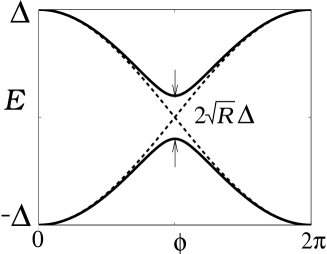
FIG. 4.: Spectrum of the Andreev levels in a QPC with finite reflectivity ($R=0.04$) (solid line), the level anticrossing is produced by electronic back scattering; at $R=0$ the Andreev levels (dashed line) coincide with the current eigen states.

It is instructive to compare the case of the transparent contact considered here with the case of a tunnel contact extensively studied in the MQC theory.[18, 19, 20] Physical difference between the two cases is that the Andreev level system in transparent contacts is a slow one, while in tunnel contacts it is a fast one because the Andreev level energy in tunnel contacts is close to $\Delta$. Within the present formalism, the integration over $\psi$ fields is similar in both cases. However, the next step, the adiabatic approximation in Eqs. (33), (34) is not allowed in the tunnel limit; instead one should perform also the integration over $\eta$ in Eq. (22), and make an expansion over small $D$. The result of this calculation, presented in Appendix A, coincides with the results of Refs. [18, 19, 34].

C Andreev levels density matrix

The Hamiltonian (40) governs the free evolution of the Andreev variable $\eta$,

$${\delta S_{\eta}^{0}\over\delta\bar{\eta}(t)}=0\,,\;\;\;i\hbar\partial_{t}\eta=h_{a}\eta.$$ (41)

The same Hamiltonian governs the free evolution of the single-particle density matrix of the Andreev levels $\rho_{a}(t)$ defined via statistical average,

$$\rho_{a}(t)=\langle\hat{\eta}(t)\hat{\eta}^{\dagger}(t)\rangle,$$ (42)

where $\hat{\eta}$ denotes the fermionic operator corresponding to the Grassmann field $\eta$, and the average is taken over all electronic states. The density matrix $\rho_{a}$ is a $2\times 2$ matrix in the Nambu space, which satisfies the normalization condition Tr$\,\rho_{a}=1$. The statistical average in Eq. (42) is represented, after the averaging over $\psi_{L,R}$, by a path integral,

$$\rho_{a}(t)=\int{\cal D}^{2}\eta\,\eta(t)\bar{\eta}(t)\,e^{iS^{0}_{\eta}/\hbar}\,.$$ (43)

Then calculating the time derivative, using Eq. (41) and the conjugated equation, we get,

$$i\hbar\partial_{t}\rho_{a}=[h_{a}\,,\rho_{a}].$$ (44)

Thus the Andreev level dynamics is described by a Liouville equation similar to ordinary quantum mechanical two-level systems.

D Andreev level current

We conclude this section with derivation of an effective current operator for the Andreev levels. A common quantum mechanical expression for the current applied to the fields $\psi_{L,R}$ at $x=\mp 0$ gives,

$$I_{L,R}(t)={e\over 2m}\left[\bar{\psi}_{L,R}(0,t)\left(-i\hbar\partial_{x}\right)\psi_{L,R}(0,t)+h.\,c.\right]\,,$$ (45)

or using Eq. (30),

$$I(t)=I_{L,R}(t)=(ie/\hbar)\sqrt{D}\,\bar{\eta}(t)\,\sigma_{z}e^{-i\sigma_{z}\phi(t)/4}\psi_{L}(0,t)\,+h.\,c.$$ (46)

[the current is continuous, $I_{L}(t)=I_{R}(t)$, by virtue of Eq. (28)]. The same equation can be obtained by varying the electronic part of the action, $S_{e}$, with respect to the phase difference,

$$I(t)={-2e\over\hbar}\frac{\delta S_{e}}{\delta\phi(t)}\,.$$ (47)

Using this relation the statistically averaged current,

$$\langle I(t)\rangle=\int{\cal D}^{2}\eta{\cal D}^{2}\psi_{L,R}\;I(t)e^{iS_{e}/\hbar}\,,$$ (48)

can be written as

$$\langle I(t)\rangle=2ei\frac{\delta}{\delta\phi(t)}\int{\cal D}^{2}\eta{\cal D}^{2}\psi_{L,R}\;e^{iS_{e}/\hbar}\,,$$ (49)

or, after tracing out the fields, $\psi_{L,R}$,

$$\langle I(t)\rangle=2ei\frac{\delta}{\delta\phi(t)}\int{\cal D}^{2}\eta\;e^{iS_{\eta}^{0}/\hbar}\,.$$ (50)

This leads to the following equation for the current in terms of the Andreev variable,

$$I(t)={-2e\over\hbar}\frac{\delta S^{0}_{\eta}}{\delta\phi(t)}=\bar{\eta}(t)\,I\,\eta(t)\,,$$ (51)

in which the kernel $I$ corresponds to the effective single particle current operator of Andreev levels,

$$I=\frac{2e}{\hbar}\frac{dh_{a}}{d\phi}=-\frac{e}{\hbar}{\cal I}(\phi)\,e^{-i\sigma_{x}\sqrt{R}\phi/2}\,\sigma_{z}\,,\;\;\;{\cal I}(\phi)=\Delta D\sin\frac{\phi}{2}.$$ (52)

Apparently the current operator does not commute with the Andreev level Hamiltonian, $[h_{a}\,,\,I]\neq 0$, which is the consequence of a normal electron reflection at the QPC. Hence the Andreev level eigen states consist of superpositions of the current eigen states, unless $R=0$ (see Fig. 4). Correspondingly, the Andreev level current, defined as an expectation value of the current operator over the Andreev state,

$$I_{a}=\langle I\rangle_{a}=\pm{2e\over\hbar}{dE_{a}(\phi)\over d\phi}=\mp{eD\Delta^{2}\over 2\hbar E_{a}}\sin\phi,$$ (53)

differs from the current eigenvalues, $\mp e{\cal I}/\hbar$ [$\langle...\rangle_{a}$ denotes averaging over the Andreev level eigenstate]. Thus the Andreev level current undergoes strong quantum fluctuations. The spectral density of current-current correlation function can be directly calculated by using Eqs. (40) and (52), [cf. Ref.[35]],

$$S(\omega)=\langle I\rangle_{a}^{2}R\tan^{2}(\phi/2)\,\delta(\omega-2E_{a}/\hbar).$$ (54)

IV Averaging over phase fluctuations

Equation (44) describes dynamics of the Andreev levels for a given realization of the time dependent phase across the QPC. However, the phase dynamics is strongly coupled to the Andreev levels. Intrinsic dynamics of the phase is governed by the quantum Hamiltonian of the loop oscillator [cf. Eq. (16)],

$$H_{osc}={p^{2}\over 2M}+{M\omega_{p}^{2}\tilde{\phi}^{2}\over 2}\;,\;\;[\,p,\phi\,]=-i\hbar\;,\;\;M={\hbar^{2}\over 8E_{C}},$$ (55)

where $\omega_{p}=\sqrt{8E_{L}E_{C}/\hbar^{2}}$ is a plasma frequency of the oscillator determined by the contact charging energy, $E_{C}=e^{2}/2C$, and the loop inductive energy, $E_{L}=(\hbar c/2e)^{2}(1/L)$. Thus the whole system is generally a multilevel one. On the other hand, the phase dynamics and the coupling between the loop oscillator and the Andreev levels is a vital part of the ALQ operation: The Andreev levels cannot be manipulated if the phase dynamics was frozen because any manipulation requires variation of the current, and second, the read out of the Andreev levels can be only performed via measuring the quantum state of the loop oscillator. An obvious way to solve this problem and preserve the qubit property of the coupled system is to ”enslave” the loop oscillator by choosing the oscillator level spacing $\hbar\omega_{p}$ much larger than the Andreev level spacing, $\hbar\omega_{p}\gg 2E_{a}$. Then the Andreev state evolution will not excite the oscillator, which will remain in the ground state and adiabatically follow the evolution of the Andreev levels. This implies that the phase is a fast variable which should be averaged out, leading to an effective qubit Hamiltonian.

FIG. 5.: Potential energy diagram for two displaced oscillator states corresponding to the different current states in the point contact (shown as arrowed circles) . The plasma frequency, $\omega_{p}$, is large compared to the Andreev level spacing; the oscillator remains in the ground state during the qubit evolution (dashed arrow).

To facilitate the averaging procedure we take advantage of the small amplitude of the phase fluctuations, $\tilde{\phi}=\phi-\phi_{e}\ll\phi_{e}$, which was already assumed when proceeding from Eq. (35) to Eq. (37). This assumption is justified by the large inductive energy, $E_{L}\gg E_{J}\approx\Delta$, and it allows us to expand the Andreev level Hamiltonian (40) over small $\tilde{\phi}$; then proceeding to the current eigen basis, $\eta\rightarrow e^{-i\sigma_{x}\sqrt{R}\phi_{e}/4}\eta$, we get,

$$h_{a}=\Delta\,\left(\cos\frac{\phi_{e}}{2}\,\sigma_{z}+\sqrt{R}\sin\frac{\phi_{e}}{2}\,\sigma_{y}\right)-\frac{{\cal I}(\phi_{e})}{2}\,\tilde{\phi}\,\sigma_{z}\,=\,h^{0}_{a}+h_{int}\,.$$ (56)

Averaging over fast phase fluctuations can be done directly in Eq. (15) by performing explicit integration over phase. However, there is a simpler way to get the same result. Equation (44) holds for a fluctuating phase provided the oscillator is not excited. It can be viewed as the diagonal with respect to $\phi$ part of a more general equation for a full density matrix, $\rho(\sigma\phi,\sigma^{\prime}\phi^{\prime})$, for the Andreev levels plus oscillator system,

$$i\hbar\partial_{t}\rho=[h_{a}^{0}+h_{int}+H_{osc}\,,\,\rho].$$ (57)

The interaction between the Andreev levels and the oscillator given by the second term in Eq. (56) displaces the oscillator steady state from the origin by $\pm{\cal I}/2M\omega_{p}^{2}$ depending on the direction of the current in the junction or, equivalently, the state of the Andreev levels (see Fig. 5). We eliminate this term in (56) by applying the transformation,

$$h_{a}\rightarrow e^{iAp}h_{a}\,e^{-iAp}\;,\;\;A={{\cal I}(\phi_{e})\sigma_{z}\over 2M\hbar\omega_{p}^{2}}\,,$$ (58)

and then average the resulting Hamiltonian over the oscillator ground state, taking into account the relation, ${\langle e^{iA\,p}\rangle}_{0}=\exp\left(-A^{2}\,{\langle p^{2}\rangle}_{0}/2\right)$ [${\langle...\rangle}_{0}$ indicates averaging over the oscillator ground state]. As the result we get an effective Hamiltonian,

$${\langle h_{a}\rangle}_{0}=\Delta\left(\cos\frac{\phi_{e}}{2}\,\sigma_{z}+\sqrt{R^{\ast}}\sin\frac{\phi_{e}}{2}\,\sigma_{y}\right)=h_{q}(\phi_{e}),$$ (59)

where the bare contact reflectivity, $R$, is renormalized by the phase fluctuations,

$$R^{\ast}=e^{-2\lambda}R,\;\;\;\lambda={{\cal I}^{2}(\phi_{e})/4M\hbar\omega_{p}^{3}}.$$ (60)

This renormalization effect can be understood as the effect of inertia of the loop oscillator, which hinders the current variations, i.e. it works against the effect of the electronic back scattering at the contact responsible for the hybridization of the current states [see discussion in the end of the Section IIID]. The renormalization effect becomes increasingly strong in the limit of a classical oscillator with large ”mass”. Because of renormalization of the contact reflectivity, the Andreev level spectrum is modified,

$$E_{a}(\phi_{e})\rightarrow E_{a}^{\ast}(\phi_{e})=\Delta\sqrt{\cos^{2}(\phi_{e}/2)+R^{\ast}\sin^{2}(\phi_{e}/2)}\,,$$ (61)

and the qubit frequency reduces. This might be important for practical applications, because it would allow one to reduce the qubit frequency by choosing the circuit parameters rather than by tuning the contact reflectivity.

Eq. (59) gives effective Hamiltonian $h_{q}$ for the ALQ in the absence of interaction with phonons. Similarly, averaged over phase fluctuation density matrix $\langle\rho\rangle_{0}$ gives density matrix for the ALQ. Keeping the same notation, $\rho$, for the qubit density matrix, we finally arrive at the equation for the free evolution of the ALQ,

$$i\hbar\partial_{t}\rho=[h_{q}(\phi_{e})\,,\,\rho].\;\;\;$$ (62)

This equation is sufficient to describe the ALQ manipulation (by driving the biasing flux) and read out (by measuring the induced current)[1, 2], and also the qubit-qubit interaction, which is discussed in the next section.

V Inductive qubit-qubit coupling

Our treatment of the interaction of the Andreev levels with phase fluctuations can be easily extended on the case of several inductively coupled SQUIDs to describe direct qubit-qubit coupling. Let us consider as an example two SQUIDs with different QPC reflectivities, $R_{1}\neq R_{2}$, and identical circuit parameters, $C$ and $L$, mutual inductance is $\cal M$. Then the inductance terms in the Lagrangian (16) written for the two qubits will take the form,

$${1\over 2}\left({\hbar c\over 2e}\right)^{2}\,\tilde{\phi}^{T}\,\hat{L}^{-1}\tilde{\phi}\;,\;\;\;\phi=\left(\begin{array}[]{c}\tilde{\phi}_{1}\\ \tilde{\phi}_{2}\end{array}\right)\;,\;\;\;\hat{L}=\left(\begin{array}[]{cc}L&{\cal M}\\ {\cal M}&L\end{array}\right)\,,$$ (63)

where $\tilde{\phi}_{1,2}$ are fluctuating phases in the first and second qubits. By introducing the normal modes for the LC-oscillators, $\phi\rightarrow e^{-i\tau_{y}\pi/4}\phi$, we present the two-qubit Hamiltonian on the form similar to Eqs. (56), (58),

$$H=\sum_{i=1,2}\left[\Delta\,\left(\cos\frac{\phi_{e,i}}{2}\,\sigma_{zi}+\sqrt{R_{i}}\sin\frac{\phi_{e,i}}{2}\,\sigma_{yi}\right)-\frac{\tilde{\phi}_{i}}{2\sqrt{2}}\,\left(\,(-1)^{i+1}{\cal I}_{1}\,\sigma_{z1}+{\cal I}_{2}\,\sigma_{z2}\,\right)\,+\,H_{osc,i}\right]\,,$$ (64)

where $H_{osc,i}$ describes the normal oscillator with frequency $\omega_{pi}=c/\sqrt{C\,(L\pm{\cal M})}$, and the index $i=1,2$ refers to the first and second qubit. Then we apply the similar transformations as in the previous section to Eq. (64), namely, we eliminate the linear in $\tilde{\phi}_{i}$ terms by means of a canonical transformation, $H\rightarrow\exp\left(i\sum_{i}A_{i}p_{i}\right)H\exp\left(-i\sum_{i}A_{i}p_{i}\right)$, with $A_{i}=\left((-1)^{i+1}{\cal I}_{1}\sigma_{z1}+{\cal I}_{2}\sigma_{z2}\right)/(2\sqrt{2}M\hbar\omega_{i}^{2})$, and then average the transformed Hamiltonian over the ground state of the normal oscillators. As the result, we obtain an effective two-qubit Hamiltonian including direct qubit-qubit coupling,

$$H=h_{q1}+h_{q2}+(e/\hbar c)^{2}\,{\cal M}\,{\cal I}_{1}{\cal I}_{2}\sigma_{z1}\sigma_{z2}.$$ (65)

The renormalized contact reflectivities are now given by equation, $R_{i}^{\ast}=R_{i}\exp[-\left({\cal I}_{i}^{2}/4\hbar M\right)\left(\omega_{1}^{-3}+\omega_{2}^{-3}\right)]$.

It is worth mentioning that the two-qubit configuration may be also realized with a single SQUID containing QPC with two conducting modes. In this case, we have the two Andreev level Hamiltonians coupled to the same loop oscillator,

$$H=\sum_{i=1,2}\left(h_{a,i}^{0}-\frac{{\cal I}_{i}(\phi_{e})}{2}\tilde{\phi}\,\sigma_{zi}\,+\,H_{osc}\right)\,.$$ (66)

Averaging over the phase fluctuations, we arrive at the same interaction Hamiltonian as in Eq. (65) but with the loop inductance $L$ substituting for $-{\cal M}$. Thus we come to an interesting conclusion that the effect of the phase fluctuations not only reduces the bare contact reflectivity but also introduces effective coupling of the Andreev levels of different conducting modes in multimode QPC.

VI Andreev level - phonon interaction

A Effective action

In this Section we include electron-phonon interaction in the consideration. We start with the derivation of an effective action for the Andreev level-phonon interaction. To this end we repeat the calculation of the previous section adding the Lagrangian $L_{e-ph}$, Eq. (19), to Eq. (32). By keeping in the electrode Green functions only the first-order correction in small interaction constant $\gamma$, we arrive at the following action,

$$S_{\eta}=-\int dt_{1}dt_{2}\,\bar{\eta}(t_{1})\left[De^{-i\sigma_{z}\phi(t_{1})/4}G_{L}(t_{1},t_{2})\,e^{i\sigma_{z}\phi(t_{2})/4}+(1+\sqrt{R})^{2}\,e^{i\sigma_{z}\phi(t_{1})/4}G_{R}(t_{1},t_{2})e^{-i\sigma_{z}\phi(t_{2})/4}\right]\eta(t_{2})\,,$$ (67)

where the Green functions $G_{L,R}$ read,

$$G_{\alpha}(t_{1},t_{2})=\sum_{\sigma=\pm}\left[\,g_{\alpha}^{(\sigma)}(0,0;t_{1}-t_{2})+\gamma\int d{\bf r}\,|\psi_{\perp}|^{2}\int dt\,g_{\alpha}^{(\sigma)}(0,x;t_{1}-t)\,\nabla{\bf u}({\bf r},t)\,\sigma_{z}g_{\alpha}^{(\sigma)}(x,0;t-t_{2})\,\right]\,.$$ (68)

In this equation, the quantities $g_{L,R}^{(\sigma)}$ refer to the different parts, $g^{(\sigma)}(x<0,x^{\prime}<0;t)$ and $g^{(\sigma)}(x>0,x^{\prime}>0;t)$, respectively, of the translation-invariant free electron Green function, $g^{(\sigma)}(x-x^{\prime},t)$, which obeys the equation

$$\left[i\hbar\partial_{t}+\sigma\sigma_{z}vi\hbar\partial_{x}-\Delta\,\sigma_{x}\right]\,g^{(\sigma)}(x-x^{\prime},t)=\delta(x-x^{\prime})\,\delta(t)\,.$$ (69)

The Green functions $g_{\alpha}^{(\sigma)}$ in Eq. (68) are explicitly given by

$$g_{L,R}^{(\sigma)}(x,0;t)=-\Theta(\mp x)\,\frac{e^{-|x|\zeta_{t}/\hbar v}}{2\hbar v\,\zeta_{t}}\,\left[\,i\hbar\partial_{t}+\Delta\,\sigma_{x}\mp\sigma\,i\,\zeta_{t}\,\sigma_{z}\right]\,\delta(t)\,,$$ (70)

where $\zeta_{t}$ is given by the Fourier component, $\zeta_{\omega}=\sqrt{\Delta^{2}-(\hbar\omega)^{2}}$.

Proceeding to the adiabatic approximation discussed in the previous section ($\zeta_{\omega}\rightarrow\zeta_{e}$), and performing the transformation (38), we arrive at the following effective action for the Andreev level-phonon interaction,

$$S_{\eta-ph}=-\gamma\int dt\int d{\bf r}\,|\psi_{\perp}|^{2}\,n(x,t)\,\nabla{\bf u}({\bf r},t)\,,$$ (71)

where

$$n(x,t)=\frac{e^{-2|x|\zeta_{e}/\hbar v}}{4\hbar v\,\zeta_{e}}\,(1+{\rm sgn}x\,\sqrt{R})\,\Lambda(x,t)\,,$$ (72)

and

$$\Lambda(x,t)=\hbar^{2}\left(\partial_{t}\,\bar{\eta}\right)\sigma_{x}\left(\partial_{t}\eta\right)+\hbar\Delta\left(\partial_{t}\bar{\eta}\,e^{-i\sigma_{x}(\sqrt{R}-{\rm sgn}x)\phi_{e}/2}\sigma_{y}\eta+h.c.\,\right)-E_{a}^{2}\,\bar{\eta}\,\sigma_{x}\eta.$$ (73)

Taking into account the zero-order dynamic equation with respect to $\gamma$, Eq. (41), and putting $\phi=\phi_{e}$,

$$i\hbar\partial_{t}\eta=\Delta\,e^{-i\sigma_{x}\sqrt{R}\,\phi_{e}/2}\left(\cos\frac{\phi_{e}}{2}\,\sigma_{z}+\sqrt{R}\,\sin\frac{\phi_{e}}{2}\,\sigma_{y}\right)\eta\,,$$ (74)

we obtain for the quantity $n(x,t)$, Eq. (72), the following expression,

$$n(x,t)=(\sqrt{R}/2)\,\kappa\,{\rm sgn}x\,e^{-2\kappa|x|}\,\bar{\eta}\,\sigma_{x}\eta\,,$$ (75)

where $\kappa=\zeta_{e}/\hbar v$. Finally, integrating over ${\bf r}$ in the action (71), we present the effective interaction on the form,

$$S_{\eta-ph}=-\int dt\,\sum_{\bf q}\,\gamma_{\bf q}X_{\bf q}\bar{\eta}\,\sigma_{x}\eta\,,$$ (76)

where $\gamma_{\bf q}$ is the effective constant of the Andreev level-phonon coupling,

$$\gamma_{\bf q}=\gamma\kappa\,\sqrt{{\hbar\Omega_{q}R\over 2\rho Vs^{2}}}\int_{0}^{+\infty}dx\,F({\bf q}_{\perp},x)\,e^{-2\kappa x}\sin(q_{x}x)\,,\;\;\;F({\bf q}_{\perp},x)=\int d{\bf r}_{\perp}\,|\psi_{\perp}(\bf r)|^{2}\,e^{i{\bf q}_{\perp}{\bf r}_{\perp}}\,.$$ (77)

We notice that the Andreev level-phonon interaction in Eq. (76) has purely transverse origin, i.e. while inducing interlevel transitions and hence the relaxation it does not produce any additional dephasing to the one associated with the relaxation.

It is important to mention that the effective coupling constant is proportional to $\sqrt{R}$, and it turns to zero in the case of perfectly transparent constriction. This results from the already mentioned fact that the relevant phonons have small wave vectors and are not able to provide large momentum transfer ($\sim 2\hbar k$) during scattering with electrons.

The effective action in Eqs. (76) and (77) was derived for a given realization of the time dependent phase. To take into account the effect of phase fluctuation, we have to apply the transformation, Eq. (58), to the action (76); the Lagrange form of the transformation reads,

$$\eta\rightarrow\exp\left(i\,{{\cal I}(\phi_{e})\sigma_{z}\over 2\hbar}\int^{t}d\tau\tilde{\phi}(\tau)\right)\eta\,.$$ (78)

Then the integration over the phase adds the factor $e^{-\lambda}$ to the action, cf. Eq. (60), which simply implies a renormalization of the coupling constant,

$$\gamma_{\bf q}\rightarrow\gamma_{\bf q}^{\ast}=e^{-\lambda}\gamma_{\bf q}\,.$$ (79)

This result can be expected: since the Andreev level-phonon coupling is transverse in the current basis and depends on the contact reflectivity, the renormalized reflectivity $R^{\ast}$ rather than the bare one has to enter the coupling constant, $\gamma_{q}^{\ast}=\gamma_{q}(R^{\ast})$; this is consistent with Eqs. (79), (77).

B Kinetic equation

Qubit decoherence is usually described with collision terms in the Liouville equation for the qubit density matrix, which take into account interaction with an environment. Our goal now will be to derive the phonon-induced collision terms in the equation (62) for ALQ density matrix, and to evaluate the decoherence of the ALQ.

While the description of free qubit evolution was possible in the terms of the single-particle density matrix, evaluation of the collision terms goes beyond the single-particle approximation and requires the knowledge of electronic two-particle correlation functions. This is because the Andreev levels are not a rigorously isolated system but rather belong to a large fermionic system of the superconducting electrons in the contact electrodes. Thus to derive the collision terms, we apply the many-body Keldysh-Green function technique[36] combined with the path integral approach. The method described below automatically takes into account the many-body effects, namely the Pauli exclusion principle, leading to a non-linear form of the collision terms and eventually to suppression of the decoherence.

The starting point of the derivation is Eqs. (15), (22) for the propagator, in which the integration over the fast fermionic fields, $\psi_{L,R}$, and phase, $\phi$, has been performed while integration over the phonons and Andreev states remains,

$${\cal U}=\int{\cal D}\{X_{\bf q}\}\,{\cal D}^{2}\eta\,e^{iS/\hbar}\,.$$ (80)

The time evolution in the action follows now along the Keldysh contour[37] $C_{K}$, $S=\int_{C_{K}}dt\,L$, which goes from $-\infty$ to $+\infty$, and then backwards.[20, 38, 39] The interaction is supposed to be switched on and off adiabatically at the remote past, $t=-\infty$, and the phonon bath is supposed to be in the thermal equilibrium. The Lagrangian $L$ has the form,

$$L=\bar{\eta}\left(i\hbar\partial_{t}-E_{a}^{\ast}\sigma_{z}\right)\eta-\sum_{\bf q}\gamma_{\bf q}^{*}\,X_{\bf q}\,\bar{\eta}\,\sigma_{x}\eta+L_{ph}\,,$$ (81)

where $L_{ph}$ is given by Eq. (20). To reduce the time integration along the Keldysh contour to an ordinary time integral, we distinguish forward and backward branches of the contour by labeling them with index $s=1,2$, and introduce the two-component fields $\eta^{s}$ and $X_{\bf q}^{s}$. Since the action is local in time, it can be rewritten as $S=\int_{-\infty}^{+\infty}dt\,\left(L^{1}-L^{2}\right)$, where $L^{s}=L[\,\bar{\eta}^{s},\eta^{s},X_{\bf q}^{s}]$.

The first step of the derivation is to integrate out the phonon fields, which will give rise to an effective self-interaction for the field $\eta$,

$$S_{int}[\bar{\eta},\eta]=-{1\over 2}\int dtdt^{\prime}\,\left[\bar{\eta}(t)\sigma_{x}\eta(t)\right]^{s}\left[\tau_{z}\check{D}(t-t^{\prime})\tau_{z}\,\right]^{ss^{\prime}}\left[\bar{\eta}(t^{\prime})\sigma_{x}\eta(t^{\prime})\right]^{s^{\prime}}\,,$$ (82)

with the kernel $\check{D}(t-t^{\prime})$ given by

$$\check{D}(t-t^{\prime})=\sum_{\bf q}\,|\gamma_{\bf q}^{*}|^{2}\,\check{D}_{\bf q}(t-t^{\prime})\,,\;\;D_{\bf q}^{ss^{\prime}}(t-t^{\prime})=-(i/\hbar)\langle T_{C}\left(X^{s}_{\bf q}(t)\,X^{s^{\prime}}_{\bf q}(t^{\prime})\right)\rangle\,,$$ (83)

where $\check{D}_{\bf q}(t-t^{\prime})$ is the equilibrium Keldysh Green function of the phonons represented with the $2\times 2$ matrix in the Keldysh space. In these equations, $T_{C}$ is the time-ordering operator on the Keldysh contour, and $\tau_{z}$ is the Pauli matrix operating in the Keldysh space; summation over repeated indices is implied.

The next step is to take advantage of the weak electron-phonon interaction, and to decouple the four-fermionic interaction term in Eq. (82) by introducing the Hubbard-Stratonovich field ${\cal G}^{ss^{\prime}}_{\alpha\beta}(t,t^{\prime})$, which is a matrix in the Keldysh-Nambu-time space. Before doing this, it is convenient to explicitly extract the small parameter $\lambda_{ph}$, which determines the electron-phonon coupling strength, from the kernel $\check{D}$ in Eq. (82) by redefining the kernel, $\check{D}\rightarrow\lambda_{ph}\check{D}$ ($\lambda_{ph}\sim(v/s)(\omega/\omega_{D})^{2}\ll 1$, $\omega_{D}$ is the Debye frequency). As the result, we get,

$${\cal U}=\int{\cal D}\,\check{{\cal G}}\,\,{\cal D}^{2}\eta\,\exp\left[(i/\hbar)\int dtdt^{\prime}\,\bar{\eta}^{s}(t)\left[{\cal L}(t,t^{\prime})\tau_{z}-\tau_{z}\check{\Sigma}(t,t^{\prime})\tau_{z}\right]^{ss^{\prime}}\eta^{s^{\prime}}(t^{\prime})+iW[\,\check{{\cal G}}\,]\,\right]\,,$$ (84)

where ${\cal L}(t,t^{\prime})=\left(i\hbar\partial_{t}-E_{a}^{\ast}\sigma_{z}\right)\delta(t-t^{\prime})$ is diagonal in the Keldysh space, and

$$W[\,\check{{\cal G}}\,]={\hbar\over 2\lambda_{ph}}\int dtdt^{\prime}\,{\cal G}^{ss^{\prime}}_{\alpha\beta}(t,t^{\prime})\,\left[\tau_{z}\check{D}(t-t^{\prime})\tau_{z}\right]^{ss^{\prime}}\left[\sigma_{x}\,\check{{\cal G}}(t^{\prime},t)\,\sigma_{x}\right]^{s^{\prime}s}_{\beta\alpha}\,,$$ (85)

$$\Sigma^{ss^{\prime}}_{\alpha\beta}(t,t^{\prime})=i\hbar D^{ss^{\prime}}(t-t^{\prime})\left[\sigma_{x}\,\check{{\cal G}}(t,t^{\prime})\,\sigma_{x}\right]^{ss^{\prime}}_{\alpha\beta}\,.$$ (86)

Equation (84) describes dynamics of the field $\eta$ interacting with the effective field $\check{{\cal G}}$. In terms of the Keldysh-Green function for the field $\eta$,

$$G^{ss^{\prime}}_{\alpha\beta}(t,t^{\prime})=-{(i/\hbar)\langle T_{C}\left(\eta^{s}_{\alpha}(t)\,\eta^{\dagger s^{\prime}}_{\beta}(t^{\prime})\right)\rangle}\,,$$ (87)

this evolution is described by the Dyson equation,

$$\left({\cal L}\tau_{z}-\tau_{z}\check{\Sigma}[{\check{\cal G}}]\tau_{z}\right)\check{G}=\check{1}\,,$$ (88)

where the self-energy $\check{\Sigma}$ depends on the effective field $\check{{\cal G}}$. A closed equation for $\check{{\cal G}}$ can be derived by integrating out the field $\eta$ in Eq. (84). This procedure leads to the equation,

$${\cal U}=\int{\cal D}\check{{\cal G}}\,e^{iS[\,\check{{\cal G}}\,]/\hbar}\;,\;\;\;S[\check{{\cal G}}]/\hbar=-i{\rm Tr}\ln\left({\cal L}\,\tau_{z}-\tau_{z}\check{\Sigma}[\check{\cal G}]\tau_{z}\right)+W[\,\check{{\cal G}}\,]\,,$$ (89)

where ${\rm Tr}$ denotes both the matrix trace in the Keldysh-Nambu space and the integration over the time variables. Noticing that the action is large, $S[\,\check{{\cal G}}\,]\sim\lambda^{-1}_{ph}$, we evaluate the integral in Eq. (89) within the saddle-point approximation (cf. Ref. [38]). The corresponding saddle-point equation is derived by varying the action with respect to $\check{{\cal G}}$, which yields,

$$\left({\cal L}\tau_{z}-\tau_{z}\check{\Sigma}[\check{{\cal G}}]\tau_{z}\right)\check{{\cal G}}=\lambda_{ph}\check{1}.$$ (90)

Comparing Eqs. (90) and (88), we obtain the relation, $\check{\cal G}=\lambda_{ph}\check{G}$. Written in the terms of $\check{G}$,

$$\left({\cal L}\tau_{z}-\tau_{z}\check{\Sigma}[\lambda_{ph}\check{G}]\,\tau_{z}\right)\check{G}=\check{1}\,,$$ (91)

the saddle-point equation is the Dyson equation for the qubit Keldysh-Green function, Eq. (87), in which the self-energy contains only an undressed vertex part and a free phonon Green function. Including the parameter $\lambda_{ph}$ back into the kernel, $\check{D}$, $\lambda_{ph}\check{D}\rightarrow\check{D}$, we arrive at the expression for the self-energy, Eq. (86), with $\check{\cal G}$ being replaced by $\check{G}$, while $\check{D}$ is given by Eq. (83).

To proceed with the derivation of kinetic equation, it is convenient to introduce a triangular form for the Keldysh-Green function by performing transformation in the Keldysh space,

$$\check{G}\rightarrow\check{L}\tau_{z}\check{G}\check{L}^{-1}=\left(\begin{array}[]{cc}G^{R}&G^{K}\\ 0&G^{A}\end{array}\right)\;,\;\;\;\check{L}={1\over\sqrt{2}}\left(\begin{array}[]{rr}1&-1\\ 1&1\end{array}\right)\,,$$ (92)

where $G^{R(A)}=G^{11}-G^{12(21)}$ is the retarded (advanced) Green function, and $G^{K}=G^{11}+G^{22}=G^{12}+G^{21}$ is the Keldysh component. Similar relations also hold for the self-energy. Then Eq. (91) takes the form,

$$\check{{\cal L}}\,\check{G}=\check{1}+\check{\Sigma}\,\check{G}\,.$$ (93)

Kinetic equation is obtained by considering the difference between Eq. (93) and its Hermitian conjugate for the Keldysh component,[36]

$$i\hbar\left(\partial_{t}+\partial_{t^{\prime}}\right)G^{K}(t,t^{\prime})-E_{a}^{\ast}\left[\,\sigma_{z},G^{K}(t,t^{\prime})\,\right]=\left(\Sigma^{R}G^{K}-G^{K}\Sigma^{A}+\Sigma^{K}G^{A}-G^{R}\Sigma^{K}\right)(t,t^{\prime})\,.$$ (94)

The right hand side of Eq. (94) describes the qubit decoherence as well as dynamic corrections due to the phonons.[40] In the absence of the coupling to phonons, the solution of Eq. (94) has the form,

$$G^{K}_{0}(t,t^{\prime})=(-i/\hbar)\,e^{-iE_{a}^{\ast}\sigma_{z}t/\hbar}\,F\,e^{iE_{a}^{\ast}\sigma_{z}t^{\prime}/\hbar}\,,$$ (95)

where $F$ is a time-independent matrix determined by the initial state of the qubit. When a weak interaction with the phonons is switched on, an asymptotical solution to the equation (94) can be written on the form,

$$G^{K}(t,t^{\prime})=(-i/\hbar)e^{-iE_{a}^{\ast}\sigma_{z}t/\hbar}\left[\,F((t+t^{\prime})/2)+\tilde{F}(t,t^{\prime})\,\right]e^{iE_{a}^{\ast}\sigma_{z}t^{\prime}/\hbar}\,,$$ (96)

where the matrix $F$ is a slowly evolving on the time scale, $\hbar/E_{a}^{\ast}$, function of the global time $(t+t^{\prime})/2$, and $\tilde{F}$ is a rapidly oscillating small-amplitude correction (see Appendix B). Equations for the matrix elements of $F$ are derived in Appendix B, Eqs. (B14), (B15), and for the diagonal matrix elements they read,

$$\partial_{t}F_{1}=-\partial_{t}F_{2}=-{\nu\over 2}\left[\,(2N+1)\left(F_{1}-F_{2}\right)+F_{1}F_{2}-1\,\right]\,,$$ (97)

while for the off-diagonal matrix element, $F_{12}=F_{21}^{\ast}$, the equation has the form,

$$\partial_{t}F_{12}=-\left[\,{\nu\over 2}\,\left(2N+1-F_{z}\right)+2i(\delta+\delta_{0}F_{z})\,\right]F_{12}\;,\;\;\;F_{z}(t)=\left(F_{1}-F_{2}\right)/2\,,$$ (98)

where $\nu$ is the phonon-induced transition rate between the qubit levels,

$$\nu=(2\pi/\hbar)\int\frac{d^{3}q}{(2\pi)^{3}}\,V\,|\gamma_{\bf q}^{*}|^{2}\,\delta(2E_{a}^{\ast}-\hbar\Omega_{q})\,.$$ (99)

$N=\left(e^{2\beta E_{a}^{\ast}}-1\right)^{-1}$ is the phonon distribution function at the frequency equal to the qubit level spacing, $\beta=1/kT$, and $\delta$ and $\delta_{0}$ are small dynamic corrections defined in Eq. (B16).

For equal times, $t=t^{\prime}$, $G^{K}(t,t)$ is related to the qubit density matrix, Eq. (42), as follows: $G^{K}_{\sigma\sigma^{\prime}}(t,t)=(-i/\hbar)\left[\,2\rho_{\sigma\sigma^{\prime}}(t)-\delta_{\sigma\sigma^{\prime}}\right]$, and therefore Eqs. (97), (98) in fact give kinetic equation for the qubit density matrix in the interaction picture, $\tilde{\rho}=e^{i\sigma_{z}E_{a}^{\ast}t/\hbar}\rho\,e^{-i\sigma_{z}E_{a}^{\ast}t/\hbar}$, $F_{\sigma}=2\rho_{\sigma\sigma}-1$, $F_{12}=2\tilde{\rho}_{12}$. It is instructive to write Eq. (97) in terms of the qubit occupation numbers $n_{\sigma}=1-\rho_{\sigma\sigma}$,

$$\partial_{t}n_{1}=-\partial_{t}n_{2}=-\nu\left[\,(N+1)\,n_{1}(1-n_{2})\,-\,Nn_{2}\,(1-n_{1})\,\right]\,.$$ (100)

The right hand side of this equation has the standard form of the electron-phonon collision term, yielding the Fermi distribution for the equilibrium occupation numbers,

$$n_{1,2}^{0}={1\over e^{\pm\beta E_{a}^{\ast}}+1}.$$ (101)

This conclusion is consistent with the well known fact that the Fermi distribution of the Andreev levels gives correct magnitude for the equilibrium Josephson current[28, 29]. Furthermore, it follows from Eqs. (100) and (101) that ${\rm Tr}\,\rho(t)=1$. Then equations for the two independent components of the density matrix, $\rho_{z}=(\rho_{11}-\rho_{22})/2$, and $\tilde{\rho}_{12}$, omitting the dynamic corrections, read,

$$\partial_{t}\rho_{z}=-\nu\left[\,\left(2N+1\right)\rho_{z}-\rho_{z}^{2}-1/4\,\right]\,,$$ (102)

$$\partial_{t}\tilde{\rho}_{12}=-\nu\left(N+1/2-\rho_{z}\right)\tilde{\rho}_{12}\,.$$ (103)

These nonlinear equations are drastically different from the linear Bloch-Redfield equation describing decoherence of the macroscopic superconducting qubits,[22] and they have qualitatively different solutions, as illustrated in Fig. 6. Exact solutions for Eqs. (102), (103) read,

$$\delta\rho_{z}(t)=\frac{\delta\rho_{z}(0)\,e^{-\Gamma t}}{1+\delta\rho_{z}(0)\sinh(\beta E_{a}^{\ast})\left(1-e^{-\Gamma t}\right)}\,,\;\;\;\Gamma={\nu\over\sinh(\beta E_{a}^{\ast})}\,,$$ (104)

$$\tilde{\rho}_{12}(t)={\rho_{12}(0)\,e^{-\Gamma t/2}\over 1+\delta\rho_{z}(0)\sinh(\beta E_{a}^{\ast})\left(1-e^{-\Gamma t}\right)}\,,$$ (105)

where $\delta\rho_{z}(t)=\rho_{z}^{0}-\rho_{z}(t)$ is the deviation from the equilibrium, $\rho_{z}^{0}=(1/2)\tanh(\beta E_{a}^{\ast}/2)$. The evolutions of the diagonal (relaxation) and off-diagonal (dephasing) parts of the density matrix are qualitatively similar. One may distinguish the linear regime, $\delta\rho_{z}(0)\sinh(\beta E_{a}^{\ast})\ll 1$, when the decoherence is determined by the exponential law,

$$\delta\rho_{z}(t)=\delta\rho_{z}(0)\,e^{-\Gamma t},\;\;\tilde{\rho}_{12}(t)=\rho_{12}(0)\,e^{-\Gamma t/2}.$$ (106)

However, the decoherence rate, $\Gamma$, becomes exponentially small at temperature smaller than the qubit level spacing, $\beta E_{a}^{\ast}\gg 1$. At this temperature, the most interesting is the opposite, nonlinear regime, $\delta\rho_{z}(0)\sinh(\beta E_{a}^{\ast})\gg 1$. In this case, there is a wide time interval, $t\ll\sinh(\beta E_{a}^{\ast})/\nu$, where both the relaxation and dephasing follow the power law (see Fig. 6),

$$\delta\rho_{z}(t)={1\over\nu t},\;\;\;\tilde{\rho}_{12}(t)={\rho_{12}(0)\over\delta\rho_{z}(0)}{1\over\nu t},$$ (107)

and only at very large times, $t\gg\sinh(\beta E_{a}^{\ast})/\nu$, the decoherence undergoes a crossover to an exponential regime similar to Eq. (106). We note that the exponentially small relaxation rate in the linear regime is well known for the quasiparticle recombination in bulk superconductors.[41]

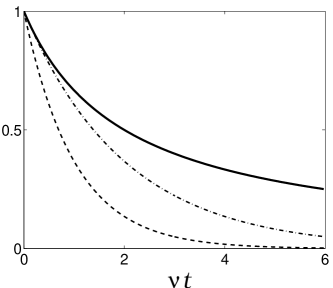
FIG. 6.: Decay with time of a ”cat” state ($\delta\rho_{z}(0)=\rho_{12}(0)=1/2$). Bold line indicates evolution of both (normalized) density matrix elements for ALQ for $1/\beta=0.2E_{a}^{\ast}$; for comparison, exponential relaxation and dephasing of a macroscopic superconducting qubit is illustrated with the dashed and dashed-dotted lines, respectively.

C Evaluation of transition rate

We conclude our study with the evaluation of the phonon-induced transition rate, $\nu$ in Eq. (99). To evaluate the transition rate, one needs to specify geometry of the junction in more detail. Let us suppose that our adiabatic constriction, Eq. (4), is formed by a hard-wall potential and has an axial symmetry. Under these assumptions, the Fourier component of transverse wave function in Eq. (77) has the form,

$$F({\bf q}_{\perp},x)=2\,{J_{1}(r_{\perp}(x)q_{\perp})\over r_{\perp}(x)q_{\perp}},$$ (108)

where $r_{\perp}(x)$ is the radius of the constriction cross section. The magnitude of the relaxation rate essentially depends on the parameter $r_{\perp}(0)Q$, where $r_{\perp}(0)$ is the radius in the neck of the constriction, and $Q=2E_{a}^{\ast}/\hbar s$ is the wave vector of phonons responsible for the interlevel transitions; for atomic-size constrictions, this parameter is small, $r_{\perp}(0)Q\ll 1$. Let us assume that the qubit level spacing is not too small, $E^{\ast}_{a}/\Delta\,\gg\,s/v$, then the phonon wave vector $Q$ is large compared to the inverse penetration length of the Andreev level wave function, $Q\gg\kappa$.

Let us for a moment assume that the Andreev level wave function does not spread out in the electrodes, but remains confined in the transverse direction, $r_{\perp}(x)=const=r_{\perp}(0)$ (see Fig. 7); then the Fourier component in Eq. (108) is close to unity, and the interaction region in Eq. (77) is limited by the penetration length of the Andreev state, $x\sim 1/\kappa$, restricting relevant phonon longitudinal wave vectors to small values, $q_{x}\sim\kappa\ll Q$. The transition rate in this case reads,

$$\nu_{0}=\frac{\gamma^{2}R^{\ast}}{16\hbar\rho s^{2}}\,\kappa Q^{2}\sim R^{\ast}(\zeta_{e}/E_{a}^{\ast})\,\tau_{ph}^{-1}(E_{a}^{\ast})\,,$$ (109)

where $\tau_{ph}^{-1}(E_{a}^{\ast})\,\sim\,E_{a}^{*3}/\hbar\Theta^{2}_{D}$ is a bulk electron-phonon relaxation rate at the Andreev level energy ($\Theta_{D}$ is the Debye temperature). This result has been derived in Ref. [32] (although neglecting the renormalization effect), and it can be qualitatively applied to long constrictions, whose length exceeds the coherence length. For short constrictions considered here, $L\ll 1/\kappa$, the effect of spreading out of the Andreev level wave function is essential, and the approximation, $r_{\perp}=const$, is not appropriate.

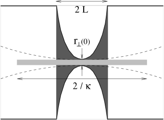
FIG. 7.: Interaction region of the Andreev levels with phonons in short QPC (dark shadow) and in long QPC (light shadow); in long QPC, increase of the constriction radius (dashed line) can be neglected.

Let us adopt the following model for the constriction shape, $r_{\perp}(x)=r_{\perp}(0)\left(1-|x|/L\right)^{-a}$, $a>1$. It is easy to see then that the integral in Eq. (77) will have a cut off at $|x|=\,L\,\ll\,1/\kappa$. Function $J_{1}(z^{a})/z^{a}$ in Eq. (108) can with good accuracy be approximated with the function, $(1/2)\,\theta(z_{0}-z)$, where $z_{0}\approx 1$, and the integral in Eq. (77) is easily evaluated, giving,

$$\nu=\kappa L\nu_{0}\,,$$ (110)

i.e., the transition rate in short constrictions significantly reduces. This is the effect due to small spatial region available for the Andreev level-phonon interaction in short QPC.

VII Conclusion

Let us summarize the outlined theory for the Andreev level qubit (ALQ). ALQ belongs to the family of superconducting flux qubits, but it differs from the macroscopic flux qubits[3, 4, 5, 6] in several important respects. First, the quantum hybridization of the flux (and persistent current) states in the ALQ loop is produced by electronic back scattering in the quantum point contact (QPC) rather than by charge fluctuations on the junction capacitors in the case of the macroscopic qubits. Thus, in principle, neither small junction capacitance nor large loop inductance is critical for the ALQ operation. Second, the ALQ is based on a QPC with large, almost full, transparency, in contrast to classical tunnel junctions employed in the macroscopic superconducting qubits. Large contact transparency is required for placing Andreev levels deep within the superconducting energy gap to achieve good decoupling from the continuum electronic states. To guarantee good separation of the qubit levels from the continuum, the amplitude of the phase fluctuations around the biasing point, $\phi\approx\pi$, must be restricted to the small values, which implies small inductance of the qubit loop.

In the tunnel junctions of the macroscopic qubits, Andreev levels are fast variables whose effect, after averaging, reduces to the Josephson potential energy added to the Hamiltonian of the loop oscillator. In the transparent junction of the ALQ, Andreev levels are slow variables which cannot be averaged out, and the full description includes the Andreev two-level Hamiltonian strongly coupled to the quantum loop oscillator. Derivation of the effective two-level Hamiltonian goes beyond the tunnel model approximation, which is done by incorporating exact boundary condition into the action of the contact.

The qubit read out is achieved via measuring fluctuating persistent current or induced flux in the qubit loop. To simplify the read out, the loop plasma frequency is chosen to be large compared to the qubit frequency so that the loop oscillator is ”enslaved” by the Andreev levels. Other regimes, e.g. resonance between the Andreev levels and loop oscillator, could be also considered, however they remained outside the scope of the paper. Typical circuit parameters for the ALQ could be chosen as follows: $E_{J}\approx\Delta$ for the single open mode, $R\leq 0.01$ with $I_{c}\sim$ 400nA for Nb; $L\sim$0.1nH, and $C\sim$ 0.1pF, giving $\omega_{p}\sim 10^{11}$sec^-1, and $E_{L}/\hbar\sim 10^{13}$sec${}^{-1}\sim 10\Delta_{Nb}/\hbar$, while $E_{a}^{\ast}/\hbar\sim 10^{10}$sec^-1.

Full description of the ALQ dynamics and qubit-qubit coupling, including qubit manipulation and read out is given by the single-particle density matrix.

Even if a good decoupling of the qubit states from the continuum electronic states is provided, there are still soft microscopic modes in the junction, which could couple to the Andreev levels. These modes present potential source of ”intrinsic” decoherence, in addition to the commonly considered external decoherence, e.g., due to fluctuating biasing and read out circuits. We considered such an intrinsic decoherence of the ALQ related to acoustic phonons. It turns out that the collision terms in the kinetic equation are nonlinear, in contrast to the linear master equation for the macroscopic superconducting qubits.[22] This reflects the fermionic nature of the Andreev states and leads to considerable enhancement of the decoherence time at small temperature. One can understand this effect in the following way. Andreev levels belong to a many-body system of superconducting electrons. Although the macroscopic behaviour of the ALQ can be expressed in terms of the single-particle density matrix, the microscopic interaction with phonons involves two-particle correlation functions, which are sensitive to the fermionic nature of the Andreev states and obey the Pauli exclusion principle. This leads to the reduced probability of the phonon-induced interlevel transitions and hence to a slower decoherence.

Furthermore, the rate of the phonon-induced transitions between the Andreev levels is significantly reduced compared to the bulk transition rate. The reason is that both the Andreev levels belong to the same normal electronic mode; this together with a rapid spreading out of the Andreev level wave function in the contact electrode strongly reduces the relevant phonon phase space.

In the paper, only the case of a single-mode QPC was considered for clarity. However, the approach might be also relevant for macroscopic Josephson qubits with tunnel junctions. In junctions with disordered tunnel barriers, the open conducting modes with large transmissivity are present.[42, 43] This introduces low-energy Andreev levels, which implies that quantum phase fluctuations become coupled to these Andreev levels, and the system must be described with the effective ALQ-type Hamiltonian. Another kind of qubits where the effective ALQ Hamiltonian might be appropriate are d-wave qubits: for the most interesting junction geometries, low-energy Andreev levels, midgap states, build up in the junction, which also makes the effective ALQ Hamiltonian to be relevant.

VIII Acknowledgement

We acknowledge useful discussions on various stages of our work with D. Khmelnitsky, Yu. Galperin, G. Johansson, A. Zaikin, L. Gorelik, R. Shekhter, I. Krive, and E. Bezuglyi. Support from EU-SQUBIT consortium, Swedish Science Foundation, SSF-OXIDE consortium, and KVA is gratefully acknowledged.

A Tunnel limit for QPC

In this Appendix, we consider a low transparency QPC, $D\ll 1$, and connect our method to the results of Refs. [18, 19] for tunnel Josephson junctions. In this limit, the Andreev levels lie very close to the edge of the superconducting gap, $E_{a}\approx\Delta$, and therefore the field $\eta$ is a fast variable, which has to be integrated out along with all the other electronic degrees of freedom. This will result in the effective action for the phase difference alone. After the integration over electronic fields, the propagator in Eq. (22) will take the form,

$${\cal U}_{e}[\phi]=\int{\cal D}^{2}\eta\,{\cal D}^{2}\psi_{L,R}\,e^{iS_{e}/\hbar}=\exp\left\{iS[\phi]/\hbar\right\}\,,$$ (A1)

$$S[\phi]/\hbar=-i{\rm Tr}\,\ln\left(1+\frac{D}{(1+\sqrt{R})^{2}}\,g^{-1}\,e^{-i\sigma_{z}\phi/2}\,g\,e^{i\sigma_{z}\phi/2}\right)\,.$$ (A2)

Here $g$ is the Green function defined in Eq. (34),

$$g(t)=-(1/\hbar v)\int_{-\infty}^{+\infty}\frac{d\omega}{2\pi}\,e^{-i\omega t}\,\frac{\hbar\omega+\Delta\,\sigma_{x}}{\sqrt{\Delta^{2}-\hbar^{2}(\omega+i\,{\rm sgn}\omega\,0)^{2}}}\,,$$ (A3)

and the matrix product in Eq. (A2) includes also the time convolutions. Taking advantage of the small $D$, and expanding the action (A2), the lowest order term reads:

$$S[\phi]/\hbar=-i(D/4)\,{\rm tr}\int_{-\infty}^{+\infty}dt_{1}dt_{2}\,g^{-1}(t_{1}-t_{2})\,e^{-i\sigma_{z}\phi(t_{2})/2}g(t_{2}-t_{1})\,e^{i\sigma_{z}\phi(t_{1})/2}\,,$$ (A4)

where the trace refers to the Nambu space. After taking the trace, the action can be written on the following form,

$$S[\phi]/\hbar=\int_{-\infty}^{+\infty}dt_{1}dt_{2}\,\left[\alpha(t_{1}-t_{2})\cos\frac{\phi(t_{1})-\phi(t_{2})}{2}+\beta(t_{1}-t_{2})\cos\frac{\phi(t_{1})+\phi(t_{2})}{2}\right]\,,$$ (A5)

with the kernels $\alpha$ and $\beta$ given by

$$\alpha(t)=i(D/2)\left(\Delta/2\hbar\right)^{2}\,\left[H_{1}^{(1)}(t\Delta/\hbar)\right]^{2}\,,$$ (A6)

$$\beta(t)=-i(D/2)\left(\Delta/2\hbar\right)^{2}\,\left[H_{0}^{(1)}(t\Delta/\hbar)\right]^{2}\,,$$ (A7)

where $H^{(1)}_{0,1}$ are the Hankel functions of the first kind. Analytical continuation to the imaginary time in Eqs. (A6) and (A7) using relation, $K_{\nu}(t)=(\pi/2)i^{1+\nu}H_{\nu}^{(1)}(it)$, leads to the same expressions for the kernels, $\alpha$ and $\beta$, as derived in Refs. [18, 19, 34], for tunnel Josephson junctions [with normal resistance of the tunnel junction being replaced with the normal resistance of the single-channel QPC: $R_{N}=(De^{2}/\pi\hbar)^{-1}$].

For a slow varying phase, $\phi$, on the time scale of the kernel variations, $\hbar/\Delta$, the both cosine terms in Eq. (A5) can be expanded over the relative time coordinate, $\tau=t_{1}-t_{2}$, up to the second order, and the effective action takes a simpler form,

$$S[\phi]=\int dt\,\left[\frac{\delta C}{2}\left(\frac{\hbar\dot{\phi}}{2e}\right)^{2}+{\hbar\over 2e}I_{c}\cos\phi\right]\,,$$ (A8)

where $I_{c}=2e\int_{-\infty}^{+\infty}d\tau\,\beta(\tau)=eD\Delta/2\hbar$ is the critical Josephson current of the single-channel tunnel point contact, and

$$\delta C(\phi)=-\frac{e^{2}}{\hbar}\int_{-\infty}^{+\infty}d\tau\,\tau^{2}\left[\,\alpha(\tau)-\beta(\tau)\cos\phi\,\right]=\frac{3}{32}\frac{De^{2}}{\Delta}\left[\,1-(1/3)\cos\phi\,\right]$$ (A9)

is the correction to the contact capacitance due to the quasiparticle tunneling.[34, 19]

B Derivation of kinetic equation

In this Appendix we derive Eqs. (97), (98) from the equation for the Keldysh function, Eq. (94). It is convenient to write the equation in the mixed representation,

$$i\hbar\partial_{t}G^{K}_{\omega}(t)-E_{a}^{\ast}\left[\,\sigma_{z},G^{K}_{\omega}(t)\,\right]=\left(\,\Sigma^{R}\,G^{K}-G^{K}\,\Sigma^{A}+\Sigma^{K}\,G^{A}-G^{R}\,\Sigma^{K}\,\right)_{\omega}(t)\,,$$ (B1)

where

$$\check{G}_{\omega}(t)=\int d\tau\,e^{i\omega\tau}\,\check{G}(t+\tau/2,t-\tau/2)\,,$$ (B2)

and the products include the convolutions defined by the equation,

$$\left(\,A\,B\,\right)_{\omega}(t)=\int\frac{d\omega_{1}d\omega_{2}}{(2\pi)^{2}}\int d\tau_{1}d\tau_{2}\,e^{i\left[(\omega-\omega_{1})\tau_{2}+(\omega-\omega_{2})\tau_{1}\right]}\,A_{\omega_{1}}(t+\tau_{1}/2)\,B_{\omega_{2}}(t-\tau_{2}/2)\,.$$ (B3)

Neglecting effect of the phonons on the retarded and advanced Green functions of the qubit, $G^{R,A}$, we replace them in the right hand side of Eq. (B1) by the free Green functions, $G^{R,A}_{\omega}=\left(\hbar\omega-E_{a}^{\ast}\sigma_{z}\pm i0\right)^{-1}$, which are time-independent in the mixed representation. Thus, the time-dependence in the self-energy comes only from the Keldysh component, $G^{K}$. The self-energy components take the form,

$$\Sigma^{R(A)}_{\omega}(t)=(i\hbar/2)\,\sigma_{x}\int\frac{d\Omega}{2\pi}\,\left[\,D^{K}_{\Omega}\,G^{R(A)}_{\omega-\Omega}+D^{R(A)}_{\Omega}\,G^{K}_{\omega-\Omega}(t)\,\right]\sigma_{x}\,,$$ (B4)

$$\Sigma^{K}_{\omega}(t)=(i\hbar/2)\,\sigma_{x}\int\frac{d\Omega}{2\pi}\,\left(\,D_{\Omega}^{R}-D_{\Omega}^{A}\,\right)\left[\,(2N_{\Omega}+1)\,G^{K}_{\omega-\Omega}(t)+G^{R}_{\omega-\Omega}-G^{A}_{\omega-\Omega}\,\right]\sigma_{x}\,,$$ (B5)

where

$$D_{\Omega}^{R,A}=\int\frac{d\Omega^{\prime}}{2\pi\hbar}\,\frac{{\cal D}_{\Omega^{\prime}}}{\Omega-\Omega^{\prime}\pm i0}\;,\;\;\;D_{\Omega}^{K}=-(i/\hbar)(2N_{\Omega}+1)\,{\cal D}_{\Omega}\,,$$ (B6)

$N_{\Omega}=\left(e^{\beta\hbar\Omega}-1\right)^{-1}$ is the equilibrium phonon distribution function, and ${\cal D}_{\Omega}$ is the spectral weight function of the phonon bath,

$${\cal D}_{\Omega}=2\pi\,{\rm sgn}(\Omega)\sum_{\bf q}\,|\gamma_{\bf q}^{*}|^{2}\,\delta(|\Omega|-\Omega_{q})\,.$$ (B7)

After integrating Eq. (B1) over $\omega$, we obtain equation for the Keldysh function at coinciding times,

$$G^{K}(t)=\int{d\omega\over 2\pi}\,G_{\omega}^{K}(t),$$ (B8)

$$i\hbar\partial_{t}G^{K}(t)-E_{a}^{\ast}\left[\,\sigma_{z},G^{K}(t)\,\right]=I_{0}+I_{1}(t)+I_{2}(t)\,,$$ (B9)

where $I_{0}=(1/2\hbar^{2})\,{\cal D}_{2E_{a}^{\ast}/\hbar}\sigma_{z}$, and

$$I_{1}(t)={-i\over 2\hbar}\int\frac{d\Omega d\omega}{(2\pi)^{2}}\int_{0}^{+\infty}d\tau\,(2N_{\Omega}+1){\cal D}_{\Omega}\left[e^{i(\omega-\Omega+E_{a}^{\ast}\sigma_{z}/\hbar)\tau}\,G^{K}_{\omega}(t-\tau/2)-e^{i(\omega+\Omega-E_{a}^{\ast}\sigma_{z}/\hbar)\tau}\,\sigma_{x}G^{K}_{\omega}(t-\tau/2)\sigma_{x}-h.c.\,\right],$$ (B10)

$$I_{2}(t)=\int\frac{d\Omega d\omega_{1}d\omega_{2}}{2(2\pi)^{3}}\int_{0}^{+\infty}d\tau\,{\cal D}_{\Omega}\left[e^{i(\omega_{2}-\omega_{1}-\Omega)\tau}\,\sigma_{x}G^{K}_{\omega_{1}}(t-\tau/2)\sigma_{x}\,G^{K}_{\omega_{2}}(t-\tau/2)+h.c.\,\right]\,.$$ (B11)

For a weak electron-phonon interaction, the right hand side of Eq. (B9) is a small perturbation, which allows one to construct an asymptotic solution by using an improved perturbation expansion,

$$G^{K}_{\omega}(t)=-(2\pi i/\hbar)\,e^{-iE_{a}^{\ast}\sigma_{z}t/\hbar}\left(F_{\omega}(\lambda t)+\sum_{n=1}^{\infty}\lambda^{n}\tilde{F}^{(n)}_{\omega}(t)\right)\,e^{iE_{a}^{\ast}\sigma_{z}t/\hbar}\,,$$ (B12)

$$F_{\omega}(t)=\delta(\omega-E_{a}^{\ast}\sigma_{z}/\hbar)\left(\begin{array}[]{cc}F_{1}(t)&0\\ 0&F_{2}(t)\end{array}\right)+\delta(\omega)\left(\begin{array}[]{cc}0&F_{12}(t)\\ F_{12}^{\ast}(t)&0\end{array}\right)\,.$$ (B13)

In Eq. (B12), $\lambda$ is a formal perturbation parameter, which reflects weak electron-phonon interaction, $\sim{\cal D}_{\Omega}$, and allows one to develop a systematic perturbative expansion. In the zero-order approximation with respect to $\lambda$, the (time-independent) matrix $F$ in Eq. (B13) is the solution of Eq. (B9) without the right hand side. The first-order equation determines the time dependence in this matrix (which absorbs formally diverging with time terms in a straightforward perturbative expansion),

$$\partial_{t}F_{1}=-\partial_{t}F_{2}=-{\nu\over 2}\left[\,(2N+1)\left(F_{1}-F_{2}\right)+F_{1}F_{2}-1\,\right]\,,$$ (B14)

$$\partial_{t}F_{12}=-\left[\,{\nu\over 2}\,\left(2N+1-F_{z}\right)+2i(\delta+\delta_{0}F_{z})\,\right]F_{12}\;,\;\;\;F_{z}(t)=\left(F_{1}-F_{2}\right)/2\,,$$ (B15)

where $\nu={\cal D}_{2E_{a}^{\ast}/\hbar}\,/\hbar^{2}$ is the phonon-induced transition rate between the qubit levels, $N=N_{2E_{a}^{\ast}/\hbar}$, and quantities

$$\delta=(1/2\hbar^{2}){\int\;\!\!\!\!\!\!\!\!-\;}\frac{d\Omega}{2\pi}\,(2N_{\Omega}+1)\frac{{\cal D}_{\Omega}}{\Omega+2E_{a}^{\ast}/\hbar}\;,\;\;\;\delta_{0}=(1/2\hbar^{2}){\int\;\!\!\!\!\!\!\!\!-\;}\frac{d\Omega}{2\pi}\,\frac{{\cal D}_{\Omega}}{\Omega+2E_{a}^{\ast}/\hbar}\,,$$ (B16)

determine the phonon-induced shift of the qubit frequency. The higher order equations determine the rapidly oscillating terms, $\tilde{F}^{(n)}_{\omega}$, in Eq. (B12); e.g., equation for $\tilde{F}^{(1)}_{\omega}$ reads,

$$\partial_{t}\tilde{F}^{(1)}={\cal I}_{z}\sigma_{z}+{\cal I}_{+}\sigma_{+}+{\cal I}_{-}\sigma_{-}\,,$$ (B17)

where $\sigma_{\pm}=(1/2)\left(\sigma_{x}\pm i\sigma_{y}\right)$,

$${\cal I}_{z}=e^{-4iE_{a}^{\ast}t/\hbar}\left(\nu/4-i\,\delta_{0}\right)F_{12}^{2}(t)+c.c.\,,$$ (B18)

$${\cal I}_{-}={\cal I}_{+}^{\ast}=e^{-4iE_{a}^{\ast}t/\hbar}\left[\,\nu\,(N+1/2)+2i\left(\delta+\tilde{\delta}_{0}\,F_{z}\right)\,\right]F_{12}(t)\;,\;\;\;\tilde{\delta}_{0}=(1/2\hbar^{2}){\int\;\!\!\!\!\!\!\!\!-\;}\frac{d\Omega}{2\pi}\,\frac{{\cal D}_{\Omega}}{\Omega}\,.$$ (B19)

It follows from these equations that $\tilde{F}^{(1)}$ indeed rapidly oscillates, with the frequency, $4E_{a}^{\ast}/\hbar$, and has relatively small amplitude, proportional to $\hbar\nu/E_{a}^{\ast}$.

REFERENCES

- [1] J. Lantz, V. S. Shumeiko, E. N. Bratus, and G. Wendin, Physica C 368, 315 (2002).
- [2] A. Zazunov, V. S. Shumeiko, E. N. Bratus’, J. Lantz, and G. Wendin, Phys. Rev. Lett 90, 087003 (2003).
- [3] C.H. van der Wal, A.C.J. ter Haar, F.K. Wilhelm, R.N. Schouten, C.J.P.M. Harmans, T.P. Orlando, Seth Lloyd, and J.E. Mooij, Science 290, 773 (2000).
- [4] J. R. Friedman, V. P. W. Chen, S. K. Tolpygo, and J. E. Lukens, Nature 406, 43 (2000).
- [5] I. Chiorescu, Y. Nakamura, C.J.P.M. Harmans, and J.E. Mooij, Science 299, 1869 (2003).
- [6] D. Vion, A. Aassime, A. Cottet, P. Joyez, H. Pothier, C. Urbina, D. Esteve, and M. H. Devoret, Science 296, 886 (2002).
- [7] V. S. Shumeiko, G. Wendin, and E. N. Bratus’, Phys. Rev. B 48, 13129 (1993).
- [8] V. S. Shumeiko, E. N. Bratus’, and G. Wendin, in Proceedings of the XXXVI Moriond Conference, Les Arcs, 2001, edited by T. Martin, G. Montambaux, and J. Tran Thanh Van (EDP Sciences, Les Ulis, France, 2001), p. 521.
- [9] B. E. Kane, Nature 393, 133 (1998).
- [10] D. Loss and D. P. DiVincenzo, Phys. Rev. A 57, 120 (1998).
- [11] N. van der Post, E. T. Peters, I. K. Yanson, and J. M. van Ruitenbeek, Phys. Rev. Lett. 73, 2611 (1994).
- [12] B. J. Vleeming, C. J. Muller, M. C. Koops, and R. de Bruyn Ouboter, Phys. Rev. B 50, 16741 (1994).
- [13] H. Takayanagi, T. Akazaki, and J. Nitta, Phys. Rev. Lett. 75, 3533 (1995).
- [14] E. Scheer, P. Joyez, D. Esteve, C. Urbina, and M. H. Devoret, Phys. Rev. Lett. 78, 3535 (1997).
- [15] B. Ludoph, N. van der Post, E. N. Bratus’, E. V. Bezuglyi, V. S. Shumeiko, G. Wendin, and J. M. van Ruitenbeek, Phys. Rev. B 61, 8561 (2000).
- [16] M. F. Goffman, R. Cron, A. Levy Yeyati, P. Joyez, M. H. Devoret, D. Esteve, and C. Urbina, Phys. Rev. Lett. 85, 170 (2000).
- [17] M. C. Koops, G. V. van Duyneveldt, and R. de Bruyn Ouboter, Phys. Rev. Lett. 77, 2542 (1996).
- [18] V. Ambegaokar, U. Eckern, and G. Schön, Phys. Rev. Lett. 48, 1745 (1982).
- [19] U. Eckern, G. Schön, and V. Ambegaokar, Phys. Rev. B 30, 6419 (1984).
- [20] G. Schön and A. D. Zaikin, Phys. Rep. 198, 237 (1990).
- [21] C. P. Slichter, Principles of Magnetic Resonance (Springer-Verlag, New York, 1990).
- [22] Yu. Makhlin, G. Schön, and A. Shnirman, Rev. Mod. Phys. 73, 357 (2001).
- [23] V. S. Shumeiko, E. N. Bratus’, and G. Wendin, Low Temp. Phys. 23, 249 (1997).
- [24] V. P. Galaiko, J. Low Temp. Phys. 26, 483 (1977).
- [25] S. A. Artemenko and A. F. Volkov, Sov. Uspekhi 22, 295 (1979).
- [26] A. G. Aronov, Yu. M. Galperin, V. L. Gurevich, and V. I. Kozub, in Nonequilibrium Superconductivity, edited by D. N. Langenberg and A. I. Larkin (North-Holland, Amsterdam, 1986), p. 325.
- [27] I. O. Kulik and A. N. Omel’yanchuk, Sov. J. Low Temp. Phys. 3, 459 (1977); 4, 142 (1978).
- [28] A. Furusaki and M. Tsukada, Physica (Amsterdam) 165B-166B, 967 (1990).
- [29] C. W. J. Beenakker and H. van Houten, Phys. Rev. Lett. 66, 3056 (1991).
- [30] D. A. Ivanov and M. V. Feigelman, Phys. Rev. B 59, 8444 (1999).
- [31] D. V. Averin, Phys. Rev. Lett. 82, 3685 (1999).
- [32] D. A. Ivanov and M. V. Feigelman, JETP Lett. 68, 890 (1998).
- [33] M. A. Desposito and A. L. Yeyati, Phys. Rev. B 64, 140511 (2001).
- [34] A. I. Larkin and Yu. N. Ovchinnikov, Phys. Rev. B 28, 6281 (1983).
- [35] A. Martin-Rodero, A. Levy Yeyati, and F. J. Garcia-Vidal, Phys. Rev. B 53, R8891 (1996).
- [36] E. M. Lifshits and L. P. Pitaevsky, Physical Kinetics (Pergamon, Oxford, 1981).
- [37] L. V. Keldysh, Sov. Phys. JETP 20, 1018 (1965).
- [38] A. Kamenev and A. Andreev, Phys. Rev. B 60, 2218 (1999).
- [39] Y. Avishai, A. Golub, and A. D. Zaikin, Phys. Rev. B 63, 134515 (2001).
- [40] J. Rammer and H. Smith, Rev. Mod. Phys. 58, 323 (1986).
- [41] S. B. Kaplan, C. C. Chi, D. N. Langenberg, J. J. Chang, S. Jafarey, and D. J. Scalapino, Phys. Rev. B 14, 4854 (1976).
- [42] K. M. Schep and G. E. W. Bauer, Phys. Rev. Lett. 78, 3015 (1997).
- [43] Y. Naveh, V. Patel, D. V. Averin, K. K. Likharev, and J. E. Lukens, Phys. Rev. Lett. 85, 5404 (2000).