High Field ESR Study of the $\pi$-d Correlated Organic Conductor
$\lambda$-(BETS)₂Fe_0.6Ga_0.4Cl₄

Abstract

Submillimeter and millimeter wave electron spin resonance (ESR) measurements of the $\pi$-d correlated organic conductor $\lambda$-(BETS)₂Fe_0.6Ga_0.4Cl₄ have been performed. Antiferromagnetic resonance (AFMR) has been observed in the insulating antiferromagnetic phase, and its frequency-field dependence can be reproduced by the biaxial anisotropic AFMR theory. We find that in this alloy system, the easy-axis is near the b-axis, unlike previous results for the pure $\lambda$-(BETS)₂FeCl₄ salts where it is closer to the c^∗-axis. We have also observed electron paramagnetic resonance (EPR) in the metallic phase at higher fields where the g-value is shown to be temperature and frequency dependent for field applied along the c^∗-axis. This behavior indicates the existence of strong $\pi$-d interaction. Our measurements further show the magnetic anisotropy associated with the anions (the D term in the spin Hamiltonian) is $|D|\sim$0.11 cm^-1.

I Introduction

The discovery of the field-induced superconductivity in $\lambda$-(BETS)₂FeCl₄, where BETS is bis(ethylenedithio)tetraselenafulvalene, by Uji et al. has attracted considerable interest since the application of a sufficiently strong magnetic field usually destroys the superconducting state.ujinature The field-induced superconducting (FISC) phase of the FeCl₄ salt appears above 17 T at a temperature of 0.1 K when the magnetic field is applied parallel to the c^∗-axis. This FISC phase can be explained by the Jaccarino-Peter compensation effect where the internal magnetic field created by the Fe³⁺ moments through the exchange interaction is compensated by the external magnetic field, and the Zeeman effect that normally destroys the superconductivity is suppressed under this condition. j-peffect ; alloy-uji ; luisprl In addition, the FeCl₄ salt shows a metal-insulator transition at $T_{MI}$=8.3 K for zero magnetic field that is associated with the antiferromagnetic ordering of the Fe³⁺ moments.brossard Therefore, the magnetic interaction between the $\pi$- and d-electrons plays an important role in these phenomena, and several electron spin resonance (ESR) measurements have been performed to probe its nature.brossard ; toyota ; isaak Electron paramagnetic resonance (EPR) and antiferromagnetic resonance (AFMR) are observed in the paramagnetic metal (PM) and antiferromagnetic insulating (AFI) phase, respectively.brossard ; toyota ; isaak Resonant features, which are related to the depolarization regime, are also observed in the canted AFI phase.isaak However, no ESR measurements (i.e. resonance experiments) have been performed in the high magnetic field region to investigate the electronic ground state in the high field metallic and FISC phases. Therefore, the purpose of the present work is to explore the electronic state of the system by covering all aspects of the phase diagram. Recent studies have shown that the FISC phase of organic alloys $\lambda$-(BETS)₂Fe_xGa_1-xCl₄ shifts to lower field as x decreases.alloy-uji Thus, we have focussed on $\lambda$-(BETS)₂Fe_0.6Ga_0.4Cl₄ where the antiferromagnetic insulating (AFI) phase exists below  6 K and  8 T, and the FISC exists above  10 T (Fig. 1), within the limits of our ESR instrumentation.

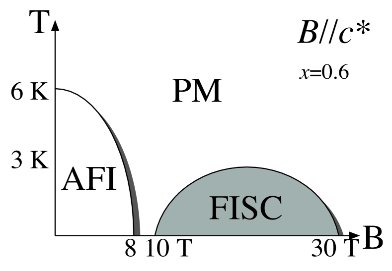
Figure 1: The phase diagram of $\lambda$-(BETS)₂Fe_xGa_1-xCl₄ (x=0.6) for B//c^∗-axis.alloy-uji PM, AFI and FISC denote paramagnetic metal, antiferromagnetic insulator and field-induced superconductor, respectively.

II Experimental

The crystal structure of the series of $\lambda$-(BETS)₂Fe_xGa_1-xCl₄ alloys has triclinic symmetry.crystal The planar BETS molecules are stacked along the a-axis and have also intermolecular interactions along the c-axis, which form a 2D electronic structure. The insulating Fe_xGa_1-xCl₄ layer is intercalated between these BETS layers. A finite exchange interaction between the $\pi$-electrons of BETS molecules and the Fe³⁺ 3d electrons (S=5/2) is expected due to the short inter-atomic distance between them. The samples are needle-shaped where the needle axis corresponds to the c^∗-axis.

ESR measurements were performed by using two different kinds of techniques. The cavity perturbation technique and the single-pass transmission technique have been used for the investigation of the low-field region (i.e. PM and AFI phase) and the high-field region (i.e. PM and FISC phase), respectively. The combination of an 8 T superconducting magnet and millimeter-wave vector network analyzer (MVNA) has been used for cavity perturbation technique.mvna The MVNA includes a tunable microwave source that covers the frequency range of 8-350 GHz, and a highly sensitive detector. The sample was set on the end-plate of the cavity so that the oscillatory magnetic field is always applied to the sample. We note that this is the usual configuration for ESR measurements. For work at higher fields and frequencies, the 25T resistive magnet and the backward wave oscillator (BWO) light source have been used with the transmission technique. The BWO can cover the frequency range from 200 to 700 GHz by using several vacuum tubes. The sample was placed in the Voigt configuration (i.e. the dc magnetic field is perpendicular to the propagation of the light) and a metallic foil was placed around the sample to mask the background radiation. The details of this high-field millimeter and submillimeter wave facility can be found elsewhere.sergei

III Results

III.1 AFI and PM phase below 8 T

Figure 2 (a) shows the temperature dependence of a typical spectra where the magnetic field is applied parallel to the c^∗-axis. The cavity perturbation technique was employed for the investigation of this low-field region. A single absorption line appears below the antiferromagnetic transition temperature $T_{AFI}$=6 K, and the resonance field shifts to lower field as the temperature is decreased. This shift indicates the evolution of the internal field below the antiferromagnetic transition. In contrast, Fig. 2 (b) shows the temperature dependence of a typical spectra where the magnetic field is applied parallel to the b-axis. Unlike the c^∗-axis results, the resonance shifts to higher field with decreasing temperature below $T_{AFI}$ which is the typical behavior of AFMR in systems with a biaxial anisotropy. The EPR above 6 K is clearly seen up to 50 K for the b-axis orientation (partially shown in Fig. 2 (b)). Although the resonance field is almost independent of the temperature, the amplitude of this absorption line decreases with the increased temperature. The EPR for B//c^∗ was not observed due to the weak intensity (expected for this orientation).

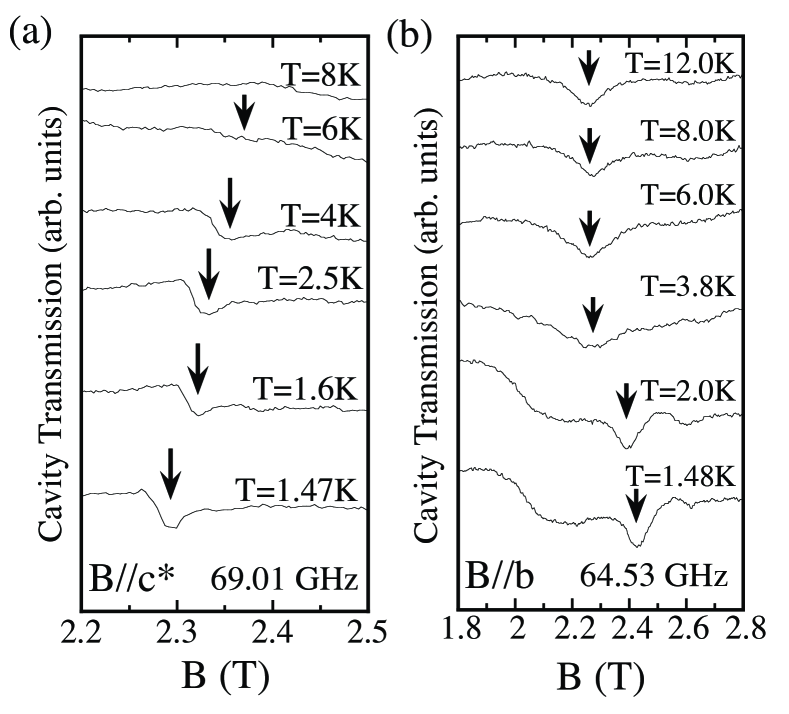
Figure 2: The temperature dependence of the ESR spectra of $\lambda$-(BETS)₂Fe_0.6Ga_0.4Cl₄ for (a) B//c^∗-axis at 69.01 GHz, and (b) B//b-axis at 64.53 GHz.

Figure 3 shows the frequency-field diagram fit with conventional AFMR theory.afmr The frequency is renormalized by the angular frequency $\omega$ divided by the gyromagnetic ratio $\gamma$ using g=2. The resonance plots are represented by triangles, circles and diamonds for B//a, b and c^∗-axes, respectively. The dotted, broken and solid lines are the theoretical curve for the easy, 2^nd easy and hard axes, respectively, where the resonance conditions are as follows:

$$\left(\frac{\omega}{\gamma}\right)^{2}_{\mathit{easy}}=B^{2}-C_{1},$$ (1)

$$\left(\frac{\omega}{\gamma}\right)^{2}_{\mathit{2^{nd}}\mathit{easy}}=B^{2}+C_{1},$$ (2)

$$\left(\frac{\omega}{\gamma}\right)^{2}_{\mathit{hard}}=B^{2}+C_{2}.$$ (3)

Here, $C_{1}$ and $C_{2}$ are the parameters $\sqrt{C_{i}}=\sqrt{2H_{E}H^{i}_{A}}$ (i=1,2), and $H_{E}$, $H^{1}_{A}$, and $H^{2}_{A}$ represent the exchange field, and the anisotropy fields for the intermediate and hard axis, respectively. The spin-flop field $B_{sf}$, equal to $\sqrt{C_{1}}$, can be obtained from the fitted parameters. The resonance plots are best fit with $\sqrt{C_{1}}$= $B_{sf}$ =0.9 T and $\sqrt{C_{2}}$=1.1 T for 1.5 K, where the difference between these two values indicates that the spin system takes a biaxial anisotropy which is consistent with similar findings for the pure FeCl₄ salt.toyota However, our results show that the easy axis is close to the b-axis, contrary to the pure FeCl₄ salt results where the easy axis is near the c^∗-axis.brossard ; toyota ; isaak We note that we could not observe AFMR near the spin-flop field $B_{sf}$ with X-band ESR measurements.

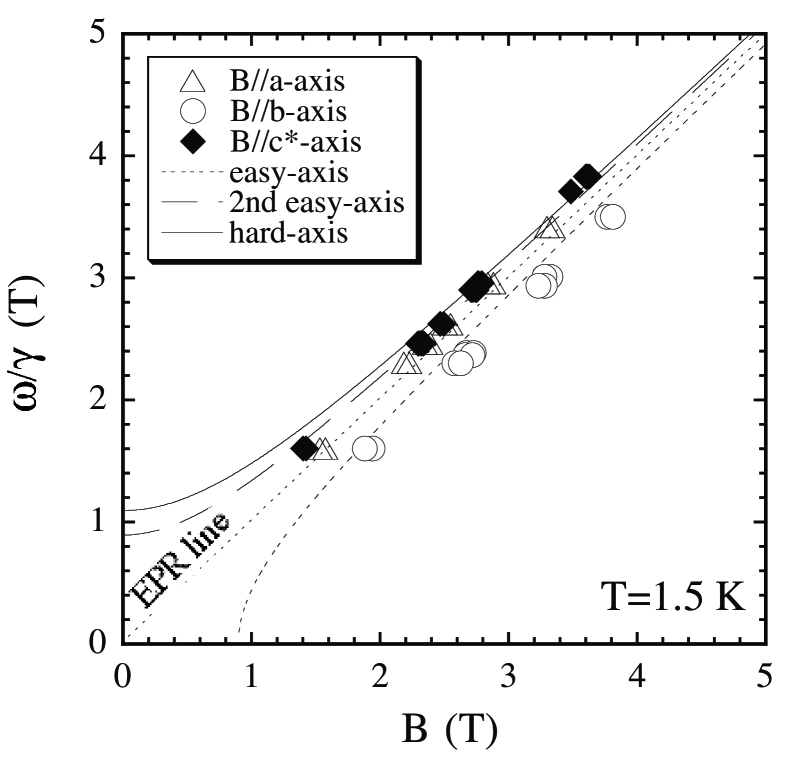
Figure 3: The frequency-field diagram of the observed AFMR at 1.5 K fitted with the theoretical AFMR curves. (See text for details.)

III.2 FISC and PM phase above 8 T

To explore the high field ground states, we employed the single-pass transmission spectroscopy technique in combination with the 25 T resistive magnet, which covers the PM phase and the FISC phase. Typical spectra at $\sim$2 K with the magnetic field applied parallel to the c^∗-axis are shown in Fig. 4. Each spectrum is renormalized since the power of the light source depends on the observing frequency. Two absorption lines are observed, one with a broad linewidth and the other with a sharp linewidth, represented by triangles and open circles in Fig. 4, respectively. We note that the frequency 298.0 GHz corresponds to $\sim$10 T when g=2 which corresponds to the boundary of the FISC phase (see Fig. 1). Therefore, for higher frequencies, the ESR at low temperatures is measured in the FISC phase. As shown in Fig. 4, although the sharp absorption line intensity and linewidth become weaker and broader, the broad absorption lines do not change as the observing frequency increases. Moreover, the effective g-value of the sharp absorption depends on frequency, while the broad one does not (see the inset of Fig. 4). The details of these absorption lines will be discussed in the next section.

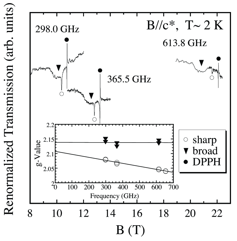
Figure 4: ESR spectra of $\lambda$-(BETS)₂Fe_0.6Ga_0.4Cl₄ at high magnetic fields. The inset shows the frequency dependence of the effective g-value for the sharp (open circle) and broad (triangle) absorption lines. The sharp absorption represented by the solid circle is DPPH, used as a field marker.

Figure 5 shows the temperature dependence of ESR spectra for 298.0 GHz for B//c^∗-axis. Although the broad absorption line is almost independent of temperature, the sharp absorption line appears around 30 K and shifts gradually as the temperature decreases. The same behavior is also observed in the higher frequency data. The sharp absorption intensity increases as the temperature is decreased, which means the sharp absorption is EPR.

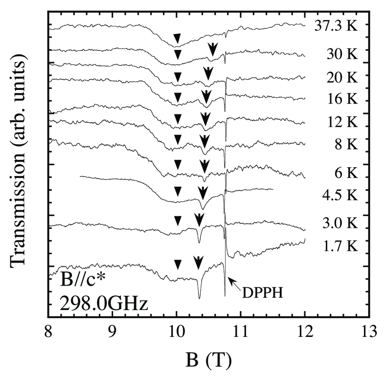
Figure 5: The temperature dependence of the typical spectra for $\lambda$-(BETS)₂Fe_0.6Ga_0.4Cl₄ at high magnetic field. The sharp and broad absorption lines are represented by the arrow and triangle, respectively.

IV Discussion

In this section, we discuss the nature of the ground state of $\lambda$-(BETS)₂Fe_0.6Ga_0.4Cl₄ and the specific details of its phase diagram, as probed by the ESR study.

IV.1 AFI phase

In the AFI phase, we have observed AFMR which can be described by the biaxial AFMR theory and we have obtained two parameters, $\sqrt{C_{1}}$= $B_{sf}$ =0.9 T and $\sqrt{C_{2}}$=1.1 T. The spin-flop field $B_{sf}$ is consistent with the magnetic susceptibility results of $\lambda$-(BETS)₂Fe_xGa_1-xCl₄ where $B_{sf}$ is 0.7 T and 0.75 T for x=0.55 and x=0.7, respectively.alloy-akane The exchange field $H_{E}$ can be given by $H_{E}=AM_{0}$ where A is the molecular field coefficient and $M_{0}$ is the magnitude of the sublattice moment in the antiferromagnetic state. These values can be obtained from the following relationships,

$$A\sim 1/\chi_{\mathit{peak}},$$ (4)

$$M_{0}=\frac{N}{2}g\mu{{}_{B}}S,$$ (5)

where $\chi_{\mathit{peak}}$ is the magnitude of the magnetic susceptibility peak and N is number of spins. The susceptibility of $\lambda$-(BETS)₂Fe_xGa_1-xCl₄ at $T_{N}$ is around 0.22 emu/mol, which is relatively high for organic conductors.alloy-akane ; alloy-akutu This is due to the contribution of the magnetic Fe³⁺ moments. If we assume that g and S are 2 and 5/2, respectively, the obtained exchange field is $H_{E}\sim$6.3 T which is similar value to the pure FeCl₄ salts.brossard The relation between the exchange field $H_{E}$ and the exchange interaction J can be expressed by

$$H_{E}=\frac{2zJS}{g\mu{{}_{B}}},$$ (6)

where z is the number of the nearest-neighbor spins. If we assume that the nearest-neighbor for Fe³⁺ moments is 2 along the a-axis,brossard ; crystal then the value of J is obtained to be 0.8 K, which is in a good agreement with the exchange interaction $J_{d}$ calculated from mean-field theory.mori If we use $H_{E}\sim$6.3 T, the anisotropy field $H^{1}_{A}$ and $H^{2}_{A}$ can be obtained from $C_{1}$ and $C_{2}$ , respectively, as mentioned in Sec. 3. Then we obtain $H^{1}_{A}$=38 mT, $H^{2}_{A}$ =64 mT. The exchange field is found to be much larger than the anisotropy fields, $H^{i}_{A}$ (i=1,2) $\ll H_{E}$, which is consistent with the appearance of the spin-flop transition.alloy-akane The anisotropy field ratio of $H^{2}_{A}/H^{1}_{A}$ is about 2. We note that the values of $H_{E}$, $H^{1}_{A}$, and $H^{2}_{A}$ for pure FeCl₄ salts obtained by Suzuki et al. are 1-2 orders different from our results.toyota This difference arises from the assumption that the AFMR comes from the spin wave excited in the $\pi$ spin system or d spin system. Although the strong interaction between $\pi$-$\pi$ and $\pi$-d electrons can not be ignored, it is difficult to explain the high magnetic susceptibility of this material at $T_{N}$ if the exchange field is 2 orders higher than our result.

In principle, the intensity of EPR just above $T_{N}$ is comparable to the intensity of AFMR as observed in Fig. 2 (b). Since the EPR is likely to originate from Fe³⁺ due to the large magnetic moment, the AFMR should also involve the d-electrons. It is also important to note that usually the resonances from $\pi$- and d-electrons merge into one resonance due to the exchange interaction between them. The resonances can be split when the Zeeman energy exceeds the exchange interaction, $2J\sim\Delta g\mu{}_{B}H$ where $\Delta g$ is the difference of the g-values between the two spins.exchangenarrow The exchange interaction J_π-d is estimated to be $\sim$15 K for FeCl₄ salts.mori Then the Zeeman energy is around 625 GHz which is much higher than the observing frequency. Therefore, the resonances should combine as one resonance which is predominantly from the S=5/2 d-electrons, especially at low temperature.

We have found that the easy-axis is near the b-axis, based on our fit to the AFMR theory as shown in Fig. 3. This is distinct from the results for the pure FeCl₄ salt where the easy-axis is found to be in a direction tilted by 30^∘ from c- to b^∗-axes.toyota ; torque1 ; torque2 The Fe³⁺ content of the alloy we have investigated is 40 % less than the pure FeCl₄ salt. This implies that the distances between d-electrons are, on average, larger, and this may be the reason for the easy-axis difference. In fact, from studies of the spin-Peierls compound CuGeO₃,cugeo3 it is well-known that doping can significantly affect the magnetic anisotropy (Ref. 18 and Refs. therein). The easy-axis is probably not exactly along the b-axis since there is some uncertainty in the theoretical fits in Fig. 3, particularly at low frequencies. Angular dependent torque measurements would be useful to determine the exact direction of the easy-axis, and to follow the change of easy-axis direction systematically with the Fe³⁺ concentration.

IV.2 PM and FISC phases

We now discuss the EPR observed in the high field region. Two absorption lines have been observed where the broad signal is independent of temperature, and the sharp signal is temperature and frequency dependent. Here the magnetic field is aligned along the c^∗-axis. Surprisingly, the two EPR absorption lines are still observed at 2 K in the FISC state, as shown in Figs. 1 and 4. Normally, the ESR measurement in a superconductor becomes difficult due to the limitation of the penetration depth $\lambda$. Although the penetration depth for this system is unknown, there should be some penetration of the magnetic flux if we consider that the Jaccarino-Peter compensation effect takes place. In this case, the magnetic field should be inhomogeneous, which might cause linewidth broadening or a g-shift of the observed absorption. As mentioned above, the sharp absorption becomes broader and its g-value is changing as the frequency increases at $\sim$2 K (see Fig. 4). The intensity of the sharp signal also decreases. However, the temperature dependence of the linewidth and the g-value do not change significantly at the phase boundary, as shown in Fig. 5. This suggests that the behavior of the sharp resonance (i.e. linewidth broadening and g-shift at $\sim$2 K) is not related to the FISC state. We think that the sample is only partially superconducting at $\sim$2 K and the resonance is coming from paramagnetic domains.

The shift of EPR line versus the temperature, which is known as the g-shift, usually occurs as a result of the spin-orbit interaction. However, in the case of magnetic metals, the interaction between the conduction electron and the localized spins (i.e. $\pi$-d interaction) also causes a g-shift. Therefore, it is possible that the $\pi$-d interaction J_π-d increases at lower temperature, leading to the g-shift of the EPR line. According to the basic ESR theory of magnetic ions in metals, the temperature dependence of the linewidth and the g-shift can be expressed as

$$\Delta{}H=A+BT,$$ (7)

$$\Delta{}g=J_{\pi{}-d}D(E_{F}),$$ (8)

respectively.s-desr Here, $D(E_{F})$ is the density of state at the Fermi level, A is a residual linewidth, and B is given by

$$B=\frac{k_{B}\pi(\Delta{}g)^{2}}{g_{\pi}\mu{{}_{B}}},$$ (9)

known as the “Korringa relation”. Figure 6 shows the temperature dependence of the effective g-value and linewidth for the sharp absorption. A linear fit to the linewidth yields A=0.05 T and B=4.8$\times$10^-3 T/K. If we assume the g-value of the $\pi$-electrons is $g_{\pi}$=2 and use the parameter B in Eq. 9, we obtain $\Delta{}g$=0.05 which is in good agreement with our results of Fig. 6. However, this is not the case if we derive the $\pi$-d exchange interaction from Eq. 8. If we estimate the density of states at Fermi level $D(E_{F})$ to be 1.2$\times$10²² J^-1 from the specific heat measurements,hinetu then J_π-d becomes 8 mK, which is not consistent with the theoretical value.mori This discrepancy comes from the so-called “bottleneck effect” where J_π-d is often underestimated.s-desr In the present case, we assume an effective g-value of combined $\pi$- and d-electron spins. Although the intensity of the conduction electron spin resonance is temperature independent in response to the Pauli spin susceptibility, the spin susceptibility of localized d-electron increases with decreasing temperature. Therefore, the effective g-value usually passes from that for conduction electrons at high temperatures to that for localized spins at lower temperatures.s-desr The behavior in Fig. 5 is consistent with this prediction (i.e. the g-value is close to 2 at high temperature) and suggests the presence of non-negligible $\pi$-d interactions in the system.

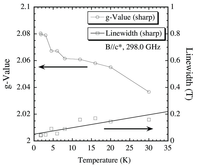
Figure 6: The temperature dependence of the effective g-value and the linewidth taken from the sharp absorption observed in Fig. 5.

The frequency dependence of the effective g-value for the sharp absorption line is also of note (see inset of Fig. 4). To explain this behavior, we have considered a system where the spins of $\pi$- and d-electrons, $S_{\pi}$=1/2 and $S_{d}$=5/2, make a spin pair. In this case, the Pryce’s spin Hamiltonian can be expressed as follows,

$$H=g\mu{{}_{B}}H_{0}\left(S_{dz}+S_{\pi{}z}\right)+DS_{dz}^{2}-J\left(\mathbf{S_{d}}\cdot\mathbf{S_{\pi}}\right).$$ (10)

Here, the first term is the Zeeman part where the two spins combine to form an effective g-value. The second term is the anisotropic d-electron spin term. This term is necessary since the Cl atoms in the FeCl₄^- anion are very close to the donor BETS molecules, leading to lower symmetry in the ligand field.crystal The last term is the exchange interaction term where only the interaction between $\pi$- and d-electrons is taken into account for simplicity. If we assume $J\gg D$ and $g\mu{}_{B}H_{0}$, the combined spins S=3, 2 and the z components become good quantum numbers and we obtain 12 energy states. If we consider only the low energy state, the S=2 energy states are lower than the S=3 states when $J<0$. Then, we have

$$E_{2}=2g\mu{{}_{B}}H_{0}+\left(\frac{17}{4}\right)D+\left(\frac{7}{2}\right)J,$$

$$E_{1}=g\mu{{}_{B}}H_{0}+\left(\frac{5}{4}\right)D+\left(\frac{7}{2}\right)J,$$

$$E_{0}=\left(\frac{1}{4}\right)D+\left(\frac{7}{2}\right)J,$$ (11)

$$E_{-1}=-g\mu{{}_{B}}H_{0}+\left(\frac{5}{4}\right)D+\left(\frac{7}{2}\right)J,$$

$$E_{-2}=-2g\mu{{}_{B}}H_{0}+\left(\frac{17}{4}\right)D+\left(\frac{7}{2}\right)J.$$

Therefore, the allowed transitions $\Delta{}M=\pm 1$ in ESR are

$$h\nu{}=g\mu{{}_{B}}H_{0}+3D,$$

$$h\nu{}=g\mu{{}_{B}}H_{0}+D,$$ (12)

$$h\nu{}=g\mu{{}_{B}}H_{0}-D,$$

$$h\nu{}=g\mu{{}_{B}}H_{0}-3D.$$

The excitation from the lowest energy state is from $E_{-2}$ to $E_{-1}$ in this model, and the ESR at low temperature should mainly involve this transition, i.e. $h\nu{}=g\mu{{}_{B}}H_{0}-3D$. We show the frequency-resonance field diagram of the sharp absorption in Fig. 7. The resonance plots for B//c^∗ (open circles) and the linear fit show that there is an offset of 9.9 GHz from the origin, which is consistent with the present model. Therefore, if we take $D<0$, we obtain $|D|\sim$0.11 cm${}^{-1}\sim$ 0.16 K and g$\sim$2.01.

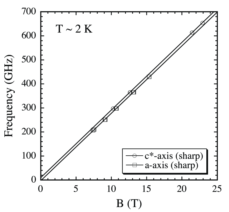
Figure 7: The frequency-field diagram of the observed EPR (sharp absorption) for B//c^∗- and a-axes.

The anisotropic D term varies with the orientation of the magnetic field. Thus, if we apply the field to the a-axis, the sharp absorption shifts to higher field as shown in Fig. 7 (rectangles). We note that this model is not limited to the $\lambda$-(BETS)₂Fe_0.6Ga_0.4Cl₄ salts, but this kind of resonance should be seen in any system where there is a non-negligible $\pi$-d interaction. Indeed, the same kind of absorption behavior is observed for (DMET)₂FeBr₄ above the saturation field.okubo In our model, the anisotropic parameter for (DMET)₂FeBr₄ would be $|D|\sim$0.3 cm^-1 for B//c^∗, which is similar to our findings for $\lambda$-(BETS)₂Fe_0.6Ga_0.4Cl₄.

Finally, we address the origin of the broad absorption line, which, unlike the sharp absorption line, does not show any significant change in g-value or linewidth. Moreover, the absorption does not shift with axis orientation. At present we have no explanation for the origin of this resonance, but it could be a result of impurities or disorder in the alloy system.

V Summary

In summary, we have performed ESR measurements on the organic $\pi$-d electron system $\lambda$-(BETS)₂Fe_0.6Ga_0.4Cl₄. The alloy system was selected so that we could carry out ESR experiments in all low temperature, field dependent ground states, including the field induced superconducting (FISC) state. We have observed AFMR and EPR for the AFI phase and PM phase, respectively. The antiferromagnetic order shows a biaxial anisotropic behavior which originates from the exchange interaction between d-electrons. The easy and hard axes correspond to the b- and c^∗-axes, respectively, and the spin-flop field is around $\sim$0.9 T. The EPR shows behavior that is related to significant $\pi$-d interaction and anisotropic Fe³⁺ magnetic moments. Due to the bottleneck effect, we could not estimate directly the exchange interaction between $\pi$- and d-electrons J_π-d. Usually, the addition of non-magnetic impurities contributes to the breaking of the bottleneck.s-desr Hence, the ESR measurements of the $\lambda$-(BETS)₂Fe_xGa_1-xCl₄ alloys with a small portion of x might be promising to estimate J_π-d. Finally, we did not observe any significant change in the EPR signal at high fields between the normal and FISC ground states. This may be a result of the nature of the FISC state, which, in the Jaccarino-Peter scenario, would allow flux to penetrate the bulk sample.

- (1) S. Uji, H. Shinagawa, T. Terashima, T. Yakabe, Y. Terai, M. Tokumoto, A. Kobayashi, H. Tanaka and H. Kobayashi, Nature 410 (2001) 908.
- (2) V. Jaccarino and M. Peter, Phys. Rev. Lett. 9 (1962) 290.
- (3) S. Uji, T. Terashima, C. Terakura, T. Yakabe, Y. Terai, S. Yasuzuka, Y. Imanaka, M. Tokumoto, A. Kobayashi, F. Sakai, H. Tanaka, H. Kobayashi, L Balicas and J. S. Brooks, J. Phys. Soc. Jpn. 72 (2003) 369.
- (4) L. Balicas, J. S. Brooks, K. Storr, S. Uji, M. Tokumoto, H. Tanaka, H. Kobayashi, A. Kobayashi, V. Barzykin and L. P. Gorkov, Phys. Rev. Lett. 87 (2001) 067002.
- (5) L. Brossard, R. Clerac, C. Coulon, M. Tokumoto, T. Ziman, D. K. Petrov, V. N. Laukhin, M. J. Naughton, A. Audouard, F. Goze, A. Kobayashi, H. Kobayashi and P. Cassoux, Eur. Phys. J. B 1 (1998) 439
- (6) T. Suzuki, H. Matsui, H. Tsuchiya, E. Negishi, K. Koyama and N. Toyata, Phys. Rev. B, 67 (2003) 020408(R).
- (7) I. Rutel, S. Okubo, J. S. Brooks, E. Jobiliong, H. Kobayashi, A. Kobayashi and H. Tanaka, Phys. Rev. B 68 (2003) 144435.
- (8) H. Kobayashi, H. Tomita, T. Naito, A. Kobayashi, F. Sakai, T. Watanabe and P. Cassoux, J. Am. Chem. Soc. 118(1996) 368.
- (9) S. Hill, N. S. Dalal and J. S. Brooks, Appl. Magn. Reson. 16 (1999)237.
- (10) S. A. Zvyagin, J. Krzystek, P. H. M. van Loosdrecht, G. Dhalenne and A. Revcolevschi, Physica B 346-347 (2004) 1.
- (11) K. Uchinokura, J. Phys.: Condens. Matter 14 (2002) R195.
- (12) T. Nagamiya, K. Yoshida and R. Kubo, Adv. Phys. 4 (1955) 1.
- (13) A. Sato, E. Ojima, H. Akutsu, Y. Nakazawa, H. Kobayashi, H. Tanaka, A. Kobayashi and P. Cassoux, Phys. Rev. B 61 (2000) 111.
- (14) H. Akutsu, K. Kato, E. Ojima, H. Kobayashi, H. Tanaka, A. Kobayashi and P. Cassoux, Phys. Rev. B 58 (1998) 9294.
- (15) T. Mori and M. Katsuhara, J. Phys. Soc. Jpn. 71 (2002) 826.
- (16) P. W. Anderson, J. Phys. Soc. Jpn. 9 (1954) 316.
- (17) J. I. Oh, M. J. Naughton, T. Courcet, I. Malfant, P. Cassoux, M. Tokumoto, H. Akutsu, H. Kobayashi and A. Kobayashi, Synth. Met. 103 (1999) 1861.
- (18) T. Sasaki, H. Uozaki, S. Endo and N. Toyota, Synth. Met.,120 (2001) 759.
- (19) R. H. Taylor, Adv. Phys. 24 (1975) 681.
- (20) E. Negishi, H. Uozaki, Y. Ishizaki, H. Tsuchiya, S. Endo, Y. Abe, H. Matsui and N. Toyota, Synth. Met. 133-134 (2003) 555.
- (21) S. Okubo, K. Kirita, Y. Inagaki, H. Ohta, K. Enomoto, A. Miyazaki and T. Enoki, Synth. Met. 135-136 (2003) 589.