Magnetoresistance of itinerant electrons interacting with local spins

Abstract

Transport properties of itinerant electrons interacting with local spins are analyzed as function of the bandwidth, $W$, the exchange interaction, $J$, and the band filling, $n$, near the band edge. Numerical results have been obtained within the dynamical mean-field approximation and interpreted with the help of analytical treatments. If spatial correlations of the magnetic fluctuations can be neglected, and defining $\rho(m)$ as the magnetization dependent resistivity, we find that $\delta\rho/\rho(0)\sim n^{-4/3}$ for $J/W,n\ll 1$ (weak coupling, low density limit), $\delta\rho/\rho(0)\sim constant$, for $J/W\gg 1,n\ll 1$ (double exchange, low density limit), where $\delta\rho=\partial\rho/\partial m^{2}|_{m^{2}\rightarrow 0}$. Possible limitations from ignoring both localization effects and critical fluctuations are also considered.

I Introduction.

A large variety of ferromagnetic materials can be described in terms of a band of itinerant electrons interacting with localized spins. Among others, we can include the manganese perovskites, La_2-xRe_xMnO₃Coey et al. (1999), the doped pyrochlores, derived from Tl₂Mn₂O₇Shimikawa et al. (1996); Martínez et al. (1999); Velasco et al. (2002), and many doped magnetic semiconductorsOhno (1998); Prinz (1998). Many of these materials show unusually large values of the magnetoresistance near the Curie temperature. The simplest description of the electronic and magnetic properties of these compounds includes an itinerant band of non interacting electrons, parameterized by the bandwidth $W$, and a finite concentration of classical localized spins, which interact with the electrons through a local exchange term, $J$. In the following, we assume that the concentration of spins is of the same order as the number of unit cells in the lattice, and describe the model in terms of two dimensionless parameters, the ratio $J/W$ and the number of electrons per unit cell, $n$. The values of these parameters for the pyrochlore compounds typically satisfy $J/W,n\ll 1$, while the double exchange model appropriate for the manganites is such that $J/W\gg 1$, and $n$ can be of order unity. The simple description used here is probably inadequate for the dilute magnetic semiconductors, where the concentration of local moments is small, and, moreover, disorder effects can lead to localization of the electronic statesCalderón et al. (2002).

It has proven useful to identify general trends in the transport properties of these materials. The resistance is typically high in the paramagnetic phase, and decreases as the magnetization increases. A simple parameter used to characterize the magnetoresistance is the dimensionless ratio ${\cal C}=[\partial\rho(m^{2})/\partial m^{2}]/\rho|_{m^{2}\rightarrow 0}$, where $\rho(m^{2})$ is the magnetization dependent resistance. The resistivity is dominated by scattering processes with wavevector $|{\bf\vec{q}}|\sim 2k_{F}$Fischer and Langer (1968), where $k_{F}$ is the Fermi momentum. The scattering arises from magnetic fluctuations, which are described by the magnetic susceptibility, $\chi({\bf\vec{q}})$. Assuming that $\chi({\bf\vec{q}})$ can be approximated taking into account only the low momentum critical fluctuations which exist near the Curie temperature, one finds that $C\propto n^{-2/3}$Majumdar and Littlewood (1998a, b).

A different regime exists at sufficiently large values of the electronic density, when $\chi(|{\bf\vec{q}}|=2k_{F})$ cannot be described in terms of critical fluctuations. In a system with a large coordination number, the properties of $\chi({\bf\vec{q}})$ for sufficiently large values of ${\bf\vec{q}}$ can be studied using an effective medium approach, which neglects the spatial correlations of the magnetic fluctuations. As it is well known, this description becomes exact when the dimensionality, or the coordination number, becomes largeGeorges et al. (1996). The conductivity of models of itinerant electrons interacting with classical spins has already been analyzed in this limitFurukawa (1994, 1995). In the following, we will study numerically the dependence of the parameter ${\cal C}$ defined above on the density of itinerant electrons, mostly in the regime when $\tilde{\epsilon}_{F}\ll W$, where $\tilde{\epsilon}_{F}$ is the Fermi energy measured from the bottom of the band, assuming uncorrelated magnetic disorder. We will perform numerical calculations in the Coherent-Potential Approximation and use simplified analytical methods to understand the numerical results. We will find that, for $J/W\ll 1$, the band splitting due to the magnetization leads to the divergent behavior, ${\cal C}\propto n^{-4/3}$. On the other hand, the magnetoresistance coefficient ${\cal C}$ remains finite close to the band edge in the double exchange limit $J/W\gg 1$, a fact easily understood in terms of a magnetization-dependent bandwidth. The paper is organized as follows. Section II presents the model and the perturbation limit for ${\cal C}$. The numerical method is described in section III. Section IV contains results for the weak coupling limit, with a simplified analytical treatment and a discussion of possible limitations due to localization effects. Results for the strong coupling limit and a simplified explanation are found in section V. The last section summarizes the main conclusions of our work and makes contact with the experimental situation, placing out results in the context of available compilations of magnetoresistance dataMajumdar and Littlewood (1998a); Velasco et al. (2002); Velasco (2002).

II Model Hamiltonian. Magnetoresistance in the perturbative limit

We consider free electrons coupled to core spins and modeled by the following Hamiltonian:

$$H=\sum_{\bf{k},\sigma}\epsilon_{\bf{k}}\>c^{\dagger}_{\bf{k},\sigma}c_{\bf{k},\sigma}-J\sum_{i}{\bf S}_{i}\cdot\mbox{\boldmath$\sigma$}_{i}$$ (1)

where $\sigma=\pm 1$ is a spin index, $\epsilon_{\bf{k}}$ is the band structure of carriers in the unperturbed system, $\mbox{\boldmath$\sigma$}_{i}$ are Pauli spin operators for carriers at site $i$, and $J$ is the coupling constant between carriers and core spins ${\bf S}_{i}$, the latter treated classically as unit length vectors ${\bf S}^{2}_{i}=1$. It should be understood from the beginning that our aim is the study of transport properties of the carriers, and not the ground state of $H$. Therefore, we consider the random distribution of core spin as given, parameterizing the problem. Consistently with the discussion of the introduction, we assume this probability distribution to be site-uncorrelated, and chosen to describe the change from a paramagnetic situation to a (weakly) ferromagnetic one. This can be achieved, for instance, with a probability ${\cal P}({\bf S})\propto\exp(h_{eff}S_{z})$. Within this parametrization, $h_{eff}=0$ corresponds to the paramagnetic phase, and $h_{eff}\neq 0$ describes a phase where the core spins are polarized along the z axis.

Following standard practice, we define the magnetoresistance coefficient, ${\mathcal{C}}$, as:

$$\frac{\rho(0)-\rho(m)}{\rho(0)}={\mathcal{C}}\>m^{2}$$ (2)

where $\rho(m)$ is the resistivity corresponding to an average polarization of core-spins $m=\langle S_{z}\rangle$. Notice that eq. 2 only makes sense to order $m^{2}$, the only situation we will consider here.

Before embarking on more complex formalisms, let us consider what perturbation theory (in the coupling $J$) has to say about the magnetoresistance. In the standard relaxation time approximation, the resistivity is given by:

$$\rho=\frac{m_{b}}{ne^{2}}\tau^{-1}$$ (3)

where $n$ is the number of carriers, $e$ the unit charge, $m_{b}$ the band mass, and $\tau$ is the relaxation time, given to lowest order in the random potential by:

$$\tau^{-1}\propto J^{2}(\langle{\bf S}^{2}\rangle-\langle{\bf S}\rangle^{2})\;{\cal D}(\epsilon_{F})$$ (4)

being ${\cal D}(\epsilon_{F})$ the density of states per spin at the Fermi level. Upon magnetizing the core spins, only changes in the fluctuating potential will modify the conductivity to order $J^{2}$. Therefore, the relevant dependence is $\tau^{-1}(m)\sim J^{2}(1-m^{2})$, leading to:

$$\frac{\rho(0)-\rho(m)}{\rho(0)}=\frac{\tau^{-1}(0)-\tau^{-1}(m)}{\tau^{-1}(0)}=m^{2}.$$ (5)

We conclude that the magnetoresistance coefficient $\mathcal{C}$ is given by

$${\mathcal{C}}=1,$$ (6)

a universal number, independent of the carrier concentration. This uninteresting results seems to preclude further consideration of the weak coupling limit, but, as we will show in the following sections, this is not the whole story. We will obtain that, close to band edges, this perturbative result fails, leading to an enhancement of $\mathcal{C}$ with decreasing carrier concentration.

III Coherent-Potential Approximation

The Hamiltonian of Eq. 1 describes non interacting electrons moving in a random potential. The obtention of electronic properties requires, therefore, performing configuration averages over the random orientation of core spins. The Coherent-Potential Approximation (CPA)Soven (1967); Taylor (1967), a procedure that we sketch here, offers a convenient way in order to obtain such averages (see, for instance, ref.Economou (1982) for coverage of the original literature). We start with the first term of Eq. 1 as our unperturbed Hamiltonian $H_{o}=\sum_{\bf{k},\sigma}\epsilon_{\bf{k}}\>c_{\bf{k},\sigma}^{\dagger}c_{{\bf k},\sigma}$, leading to a Green’s function or resolvent whose local matrix elements are given by:

$$g_{o}(z)=\langle i,\sigma|(z-H_{o})^{-1}|i,\sigma\rangle=\int d\epsilon\>\frac{{\cal D}_{o}(\epsilon)}{z-\epsilon}$$ (7)

where $|i,\sigma\rangle$ is the electron state at site $i$ and spin $\sigma$, and $z$ is a complex energy in the upper plane. This unperturbed system is characterized by a reference density of states (per spin) ${\cal D}_{o}(\epsilon)=-\pi^{-1}{\rm Im}\;g_{o}(\epsilon+i0^{+})$, which we take to be the usual semielliptical function:

$${\cal D}_{o}(\epsilon)=\frac{2}{\pi W}\sqrt{1-\left(\frac{\epsilon}{W}\right)^{2}}$$ (8)

notice that band edges are entirely consistent with a 3-d system.

The configuration average of the Green’s function for the entire $H$: $g_{\sigma}(z)=\langle\langle i,\sigma|(z-H)^{-1}|i,\sigma\rangle\rangle$ (external brackets stand for configuration average) is calculated by the CPA from that of the unperturbed system by means of a self-energy $\Sigma_{\sigma}$, in the following manner:

$$g_{\sigma}(z)=g_{o}(z-\Sigma_{\sigma})$$ (9)

where the self-energy, $\Sigma_{\sigma}(z)$, itself a function of $z$, can be thought of as providing an effective medium that substitutes the real system. This self-energy is obtained by imposing that the local scattering produced when we replace an effective site by a real one be, on the average, zero Economou (1982). Adapted to our case, the self-energy obeys the following equation (rotational symmetry around the z axis assumed):

$$\frac{1}{g_{o}(z-\Sigma_{\sigma})}=\left\langle F_{\sigma}(z,\theta)-\frac{J^{2}\sin^{2}\theta}{F_{-\sigma}(z,\theta)}\right\rangle$$ (10)

where $\cos\theta=S_{z}$, brackets stand for averages over the distribution of core spin orientations, and the auxiliary function $F_{\sigma}(z,\theta)$ is given by $F_{\sigma}(z,\theta)=\Sigma_{\sigma}+\sigma J\cos\theta+1/g_{o}(z-\Sigma_{\sigma})$, where $\sigma=+1(-1)$ for up (down) electron spin.

Although primarily intended for one-body properties (such as the density of states), the CPA can be applied to transport properties. The basic idea consists in decoupling the two-body correlations that appear in the Kubo formula into products of one-body correlators, which are then obtained with the CPA self-energy. Skipping further details, the relevant expression (see ref.Economou (1982)) adapted to our case is

$$\rho^{-1}=\sum_{\sigma}\rho^{-1}_{\sigma}$$ (11)

where the conductivity for spin $(\sigma)$ carriers, $\rho^{-1}_{\sigma}$, is given by:

$$\rho^{-1}_{\sigma}\propto\int d\epsilon^{\prime}f(\epsilon^{\prime})\left(Im\frac{1}{\epsilon_{F}+i0^{+}-\Sigma_{\sigma}(\epsilon_{F}+i0^{+})-\epsilon^{\prime}}\right)^{2}$$ (12)

where $\epsilon_{F}$ is the Fermi level and the function $f(\epsilon^{\prime})\propto(1-(\epsilon^{\prime}/W)^{2})^{3/2}$ accounts for matrix elements of the velocity operatorEconomou (1982); Chattopadhyay et al. (2000).

The whole CPA procedure for transport properties can be considered as a mean-field approximation. Actually a double mean-field: first for the resolvent and later for transport (decoupling). Therefore, its main shortcoming will be fluctuation related effects (i.e. localization). Nevertheless, we expect the 3-d nature of our problem to mitigate this limitation. In fact, the CPA has been shown to provide a good description of 3-d disordered systems, being one of the very few non perturbative methods available. In recent times, this approximation is often termed dynamical mean fieldGeorges et al. (1996), an approach invented for genuine many body problems that becomes equivalent to the CPA when applied to a Hamiltonian like that of eq. (1).

IV Results. Weak coupling limit: $J/W<<1$

We have calculated the magnetoresistance coefficient by direct numerical subtraction of the CPA conductivities in the paramagnetic and ferromagnetic cases, the latter induced with a tiny effective field in the probability distribution for core spins: ${\cal P}({\bf S})\propto\exp(h_{eff}S_{z})$. Representative results for coupling constants well below the bandwidth $(J<<W)$ are shown in fig. 1, where the magnetoresistance coefficient $({\mathcal{C}})$ is plotted versus carrier density per site $(n)$. Notice that, in this weak coupling regime, the perturbative value ${\mathcal{C}}=1$ is closely approached over most of the concentration range. Yet, significant enhancement of ${\cal C}$ is evident for small carrier concentration, that is, close to the band edge. The inset of fig. 1 blows up the low density regime, where values of ${\mathcal{C}}>100$ are easily obtained. In fact, our numerical results are compatible with a divergent behavior of ${\mathcal{C}}$ in that limit. Fig. 1 is representative of the small coupling regime $J<<W$: no matter how weak $J$ is chosen, we can always find large enhancements of ${\mathcal{C}}$ if we approach the band edge. In fact, the smaller the value of $J$, the smaller the range of densities required to see this enhancement, as shown in the inset on fig. 1. Notice that this effect does not formally contradict the perturbative result: for fixed carrier density (i.e. fixed Fermi level), ${\mathcal{C}}\rightarrow 1$ when $J\rightarrow 0$. Nevertheless, the quantitative failure of the perturbative results for a given $J$ seems unavoidable upon approaching the band edges. In what follows, we will address the origin of this failure with a simplified analytical procedure.

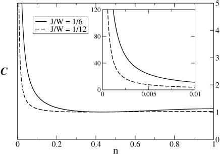
Figure 1: Magnetoresistance coefficient ${\mathcal{C}}$ (eq. 2) versus carrier density for two values of $J$. Inset: enlarged view of the low density region.

IV.1 Effect of band splitting. Analytical treatment

Our numerical results (and the analysis to follow) indicate that the nominal criterion for the validity of the perturbative result, $J<<W$, valid well within the band, has to be replaced by $J<<\tilde{\epsilon}$, where $\tilde{\epsilon}=\epsilon_{F}-(-W)$, is the distance of the Fermi level to the band edge. To see how this comes about and its effect on the magnetoresistance, the original CPA equations are rather opaque and inconvenient. Instead, we will start with the perturbative treatment of section II, adding the effect we believe is at the origin of the enhancement: band splitting. The first manifestation of a net polarization of core-spins, $m$, is a band splitting of the unperturbed density of states ${\cal D}_{o}(\epsilon\pm Jm)$. This splitting does not show up in the resistivity if one keeps the calculation to order $J^{2}$, but will affect higher order terms. The situation is depicted in fig. 2, where the up and down densities have been aligned to share a common origin, leading to different apparent Fermi levels for up and down electrons: $\tilde{\epsilon}_{\uparrow}-\tilde{\epsilon}_{\downarrow}=2mJ$. Transport properties depend on the density of states at the apparent Fermi levels which, in turn, changes rapidly upon splitting (magnetization) close to a band edge. Therefore, it is not unexpected that this mere shift can cause a large effect on the magnetoresistance. We will see that this is the case.

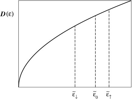
Figure 2: Schematic density of states showing the relative positions of Fermi levels upon magnetization.

We assume the simplified situation described in fig. 2 with a parabolic band ${\cal D}_{o}(\tilde{\epsilon})\sim\sqrt{\tilde{\epsilon}}$, and apply standard transport theory over this already split situation. Therefore, we have to discriminate between up and down contributions to the conductivity:

$$\rho^{-1}=\sum_{\sigma}\frac{n_{\sigma}e^{2}}{m_{b}}\tau_{\sigma}$$ (13)

where $n_{\sigma}$, is the number of carriers for each spin species, of course satisfying the constraint $n=\sum_{\sigma}n_{\sigma}$. The inverse relaxation times are given by

$$\tau_{\uparrow}^{-1}\propto J^{2}\left[{\cal D}_{o}(\tilde{\epsilon}_{\uparrow})(\langle S_{z}^{2}\rangle-m^{2})+{\cal D}_{o}(\tilde{\epsilon}_{\downarrow})\langle S_{x}^{2}+S_{y}^{2}\rangle\right]$$

$$\tau_{\downarrow}^{-1}\propto J^{2}\left[{\cal D}_{o}(\tilde{\epsilon}_{\downarrow})(\langle S_{z}^{2}\rangle-m^{2})+{\cal D}_{o}(\tilde{\epsilon}_{\uparrow})\langle S_{x}^{2}+S_{y}^{2}\rangle\right]$$

where the first contribution comes from transitions within the same spin species, and the second term accounts for spin-flip transitions (notice the different density of states in each case).

Going from the paramagnetic situation (Fermi level at $\tilde{\epsilon}_{o}$ in fig. 2) to the ferromagnetic one (Fermi levels at $\tilde{\epsilon}_{\uparrow,\downarrow}$), the magnetoresistance picks up contributions coming from changes in carrier spin populations $n_{\sigma}$ and lifetimes $\tau_{\sigma}$, in addition to the standard contribution already described in section II. Keeping consistently terms to order $m^{2}$ in eq. (13), it is only very tedious to show that the magnetoresistance coefficient can be written as :

$${\mathcal{C}}=1+\frac{19}{36}\left(\frac{J}{\tilde{\epsilon}_{o}}\right)^{2}$$ (14)

We see that it is just a matter of getting close enough to the band edge $\tilde{\epsilon}_{o}\leq J$ to obtain arbitrarily large corrections to the nominal perturbative result.

In this simplified scheme, owing to the fact that $n\sim\tilde{\epsilon}_{o}^{\;3/2}$, the magnetoresistance becomes divergent in the low carrier density with the following law:

$${\mathcal{C}}-1\sim\left(\frac{J}{W}\right)^{2}n^{-4/3}$$ (15)

This scaling seems to be obeyed by the CPA results, as illustrated in fig. 3, where the result for two values of $J<<W$ collapse onto the same straight line. This makes us believe that this simple treatment: splitting plus standard relaxation time transport, captures the essence of the enhancement observed in the CPA calculations.

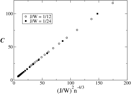
Figure 3: Magnetoresistance coefficient ${\mathcal{C}}$ versus carrier density for two values of $J$ illustrating the scaling behavior of eq. 15 in the low density limit.

IV.2 Ioffe-Regel criterion

We have seen that, for $J\ll W$, CPA calculations and the simplified treatment of Eq. (14) support the existence of a large magnetoresistance coefficient close to the band edge. In this section we address the validity of this result. The main concern comes from the fact that we have to be close to a band edge, where localization effects (ignored in our mean-field approach) are expected to play an important roleAnderson (1958); Mott (1987); Economou (1982). To estimate the energy range of this effect, we use the Ioffe-Regel criterionIoffe and Regel (1960); Mott (1987). This criterion can be stated saying that quantum corrections to transport can be expected to be relevant when the mean free path diminishes to become of the order of the de Broglie wavelength for electrons at the Fermi level. This sets a characteristic distance to the band edge $\tilde{\epsilon}_{IR}$ such that, if the Fermi level is below it, $\tilde{\epsilon}_{o}<\tilde{\epsilon}_{IR}$, localization is expected to dominate. In our case, this criterion can be written as the condition:

$$\tau^{-1}_{IR}\sim\tilde{\epsilon}_{IR},$$ (16)

where $\tau_{IR}$ is the lifetime at $\tilde{\epsilon}_{IR}$. Using the perturbative result for the lifetime, this leads to:

$$\tilde{\epsilon}_{IR}\sim 8W\left(\frac{J}{W}\right)^{4}$$ (17)

Comparing this $J^{4}$ dependence with the $J^{2}$ of Eq. (14), we see that there is ample room for observing the enhancement of ${\mathcal{C}}$ upon approaching the band edge, before the Ioffe-Regel limit is reached. More quantitatively, we can define the enhancement factor at the Ioffe-Regel limit by:

$$\Delta{\mathcal{C}}_{IR}=\frac{19}{36}\left(\frac{J}{\tilde{\epsilon}_{IR}}\right)^{2}$$ (18)

with the result that:

$$\Delta{\mathcal{C}}_{IR}\sim 10^{-2}\left(\frac{W}{J}\right)^{6}$$ (19)

Therefore, we conclude that, for our weak coupling case $J\ll W$, large increases of the magnetoresistance coefficient $\mathcal{C}$ are allowed before localization effects set in.

V Results. Double exchange limit: $J/W\gg 1$

In this limit, the splitting between the two spin subbands is large, and we can neglect the one which is at high energy, $\sim J$. We have implemented the $J=\infty$ limit in the CPA equations. A similar calculation has been carried out before by FurukawaFurukawa (1994), but here we are mainly interested in results close to the band edge. In fig. 4 we show the CPA results for the magnetoresistance coefficient ${\mathcal{C}}$ as a function of carrier density. Notice a mild enhancement of ${\mathcal{C}}$ close to the band edge but, unlike the weak coupling limit, no divergent behavior is observed. This is more clearly seen in the inset of fig. 4, where the low density region is blown up, showing a saturation of the magnetoresistance coefficient around ${\mathcal{C}}\sim 11$.

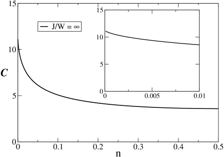
Figure 4: Magnetoresistance coefficient ${\mathcal{C}}$ (eq. 2) versus carrier density for $J/W=\infty$. Inset: enlarged view of the low density region.

Direct use of the CPA equations to understand this behavior is, again, inconvenient. A simpler picture in order to include the effect of a finite magnetization is to assume that the bandwidth depends on $m$de Gennes (1960) in the following manner: $W_{m}=W\sqrt{(1+m^{2})/2}$. This ansatz interpolates between the paramagnetic $(W_{m}=W/\sqrt{2})$ and fully ferromagnetic limit $(W_{m}=W)$, giving a reasonable approximation to the dependence of the Curie temperature on band fillingArovas et al. (1999); Guinea et al. (2000). Assuming a semielliptical density of states and measuring energies from the center of the occupied band, we have:

$${\cal D}(\epsilon)=\frac{2}{\pi W_{m}}\sqrt{1-\left(\frac{\epsilon}{W_{m}}\right)^{2}},$$ (20)

and the change in the electronic Green’s function can be described by a self-energy, $\Sigma(z,m)$, such that:

$$g(z,m)=g_{o}[z-\Sigma(z,m)]$$ (21)

with $z=\epsilon+i0^{+}$. This self-energy is:

$$\Sigma(z,m)=\frac{1-m^{2}}{2(1+m^{2})}\left[-z+\sqrt{z^{2}-W_{m}^{2}}\right]$$ (22)

We now assume that the conductivity is proportional to $n\times{\rm Im}\Sigma(\epsilon_{F},m)^{-1}$ as done in previous sections. Then:

$${\mathcal{C}}\sim-\frac{1}{{\rm Im}\Sigma(\epsilon_{F},0)}\left.\frac{\partial^{2}{\rm Im}\Sigma(\epsilon_{F},m)}{\partial m^{2}}\right|_{m^{2}\rightarrow 0}$$ (23)

In this equation we have to take into account that, if the number of particles is fixed, $\epsilon_{F}\approx W\sqrt{(1+m^{2})/2}(-1+[(3\pi)/(4\sqrt{2})]^{2/3}n^{2/3})$ has an implicit dependence on $m^{2}$. Then ${\rm Im}\Sigma\sim n^{2/3}W(1-m^{2})/\sqrt{1+m^{2}}$, and we find no divergent term in ${\mathcal{C}}$ as $n\rightarrow 0$. Therefore,

$$\lim_{n\rightarrow 0}{\mathcal{C}}\sim{\rm constant}$$ (24)

This saturation of ${\mathcal{C}}$ is obtained in the full CPA calculation (see fig. 4), lending support to this simple picture of a $m$-dependent bandwidth in the limit $J=\infty$. Notice that, for this picture to apply, the number of carriers must be kept fixed upon magnetization. If the chemical potential were kept fixed, on the other hand, we would have obtained a divergent behavior: $\lim_{n\rightarrow 0}{\mathcal{C}}\sim n^{-2/3}$.

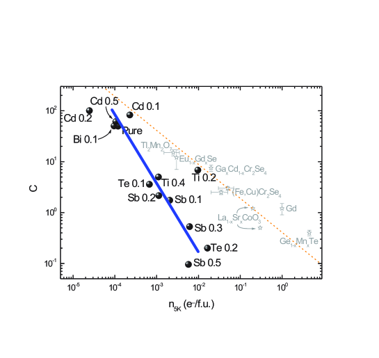
Figure 5: Value of ${\mathcal{C}}$ for the pyrochlore compounds analyzed inVelasco et al. (2002); Velasco (2002) (dark dots) and for the magnetic materials studied inMajumdar and Littlewood (1998a) (stars). The full line is a fit to a $n^{-4/3}$ dependence. The broken line is the $n^{-1/3}$ dependence discussed inMajumdar and Littlewood (1998a).

VI Validity of the approximations. Summary.

The analysis discussed above uses an effective medium approach to study the transport properties of itinerant electrons coupled to classical spins. As mentioned in the introduction, the method neglects the spatial correlations of the magnetic fluctuations: a potentially serious drawback if the source of polarization is the spontaneous magnetic order expected for the Hamiltonian of eq. 1. The critical behavior of these fluctuations is particularly important in the vicinity of the point ${\bf\vec{q}}=0$. In addition, our scheme cannot take into account the localization of the electronic states induced by the disorder in the magnetization near the band edges. Both limitations become important when the electronic density is lowered, as the relevant scattering processes are shifted towards low momenta, and the Fermi energy approaches the band edge. We will consider these two effects separately.

The lack of spatial correlations is a generic feature of effective medium theories. These correlations modify the momentum dependence of the susceptibilities at low values of the momenta. If the number of dimensions of the system were indeed large, these effects could be safely ignored, as the volume of the region near ${\bf\vec{q}}=0$ is negligible compared to the volume of the unit cell. We are interested in changes in the resistivity near the Curie temperature, so that critical fluctuations at low momenta are always present. The length scale at which these fluctuations become important is the correlation length in the paramagnetic phase, $\xi_{0}$, whereas the length scale for transport is $k^{-1}_{F}$Majumdar and Littlewood (1998b). Therefore, we expect our results to be applicable for $k_{F}\xi_{0}\gg 1$, leading to the following condition for the carrier density: $n\gg(a/\xi_{0})^{D}$, where $D$ is the dimension and $a$ the lattice size. Assuming, for instance, a typical value $\xi_{0}=5a$ and $D=3$, we find $n\geq 10^{-2}$.

Localization becomes important when the mean free path associated to the disorder, $l$ is such that $k_{F}l\sim 1$. In the weak coupling limit, its effect has been discussed before, with conclusions that we briefly repeat here. Localization is expected to be relevant below the Ioffe-Regel energy, $\tilde{\epsilon}_{IR}\sim J^{4}/W^{3}$. Therefore, observing the enhanced behavior ${\cal C}\sim n^{-4/3}$ requires the following condition on the Fermi level:

$$\frac{J^{4}}{W^{3}}\ll\tilde{\epsilon}_{F}\ll J,$$ (25)

a regime easily accessible in the weak coupling limit, $J\ll W$.

In the double exchange limit, $J/W\gg 1$, we have ${\rm Im}\Sigma\sim\sqrt{W\tilde{\epsilon}_{F}}\geq\tilde{\epsilon}_{F}$ for $n\ll 1$. The mean free path becomes comparable to the lattice spacing at low densities, implying that localization effects are relevant in this regime. Notice, though, that the applicability of the previous criterion, imported from the perturbative limit, is open to question in this strong coupling limitVarma (1996). Moreover, the use of the scheme used here to study the phase diagram shows that the paramagnetic-ferromagnetic transition becomes first order for $n\leq 10^{-1}$Arovas et al. (1999). This inclusion of this effect can change significantly the magnetoresistance.

In summary, we have studied transport properties of electrons coupled to local, uncorrelated core spins. The magnetoresistance coefficient (eq. 2) has been shown to diverge in the weak coupling limit as ${\cal C}\sim n^{-4/3}$, near the band edge, as a consequence of band splitting upon magnetization. On the other hand, the magnetoresistance remains finite in the strong coupling limit (double exchange model) close to the band edge. This is understood from a simplified picture consisting in a magnetization-modulated bandwidth. Possible limitations of the previous results from the neglect of both localization effects and critical fluctuations have been addressed.

Finally, we would like to consider the potential applicability of our results to the experimental situation. In Fig.[5], we present available informationVelasco et al. (2002); Velasco (2002) for the magnetoresistance in pyrochlores and other magnetic materials. We observe a strong dependence on the density for the pyrochlores family, which seems to come closer to the $n^{-4/3}$ law obtained in this paper than the fit based on $2k_{F}$ scattering alone Majumdar and Littlewood (1998a)

VII Acknowledgements.

We are thankful to J. L. Martínez for many helpful conversations, and to P. Velasco and J. L. Martínez for sharing with us the data shown in Fig.[5]. Financial support from MCyT (Spain), through grant no. MAT2002-04095-C02-01 is gratefully acknowledged. Additional support was provided through the France-Spain binational grant PAI PICASSO 05253WF.

References

- Coey et al. (1999) J. M. D. Coey, M. Viret, and S. von Molnar, Adv. in Phys. 48, 167 (1999).
- Shimikawa et al. (1996) Y. Shimikawa, Y. Kubo, and T. Manako, Nature 379, 53 (1996).
- Martínez et al. (1999) B. Martínez, R. Senis, J. Fontcuberta, X. Obradors, W. Cheikh-Rouhou, P. Strobel, C. Bougerol-Chaillout, and M. Pernet, Phys. Rev. Lett. 83, 2022 (1999).
- Velasco et al. (2002) P. Velasco, J. A. Alonso, M. T. Casais, M. J. Martínez-Lope, J. L. Martínez, and M. T. Fernández-Díaz, Phys. Rev. B 66, 174408 (2002).
- Ohno (1998) H. Ohno, Science 281, 951 (1998).
- Prinz (1998) G. A. Prinz, Science 282, 1660 (1998).
- Calderón et al. (2002) M. J. Calderón, G. Gómez-Santos, and L. Brey, Phys. Rev. B 66, 075218 (2002).
- Fischer and Langer (1968) M. E. Fischer and J. S. Langer, Phys. Rev. Lett. 20, 665 (1968).
- Majumdar and Littlewood (1998a) P. Majumdar and P. B. Littlewood, Nature 395, 479 (1998a).
- Majumdar and Littlewood (1998b) P. Majumdar and P. Littlewood, Phys. Rev. Lett. 81, 1314 (1998b).
- Georges et al. (1996) A. Georges, G. Kotliar, W. Krauth, and M. Rozenberg, Rev. Mod. Phys. 68, 13 (1996).
- Furukawa (1994) N. Furukawa, J. Phys. Soc. Jpn 63, 3214 (1994).
- Furukawa (1995) N. Furukawa, J. Phys. Soc. Jpn 64, 2734 (1995).
- Velasco (2002) P. Velasco, Ph.D. thesis, Universidad Autónoma de Madrid (2002).
- Soven (1967) P. Soven, Phys. Rev. 156, 809 (1967).
- Taylor (1967) D. W. Taylor, Phys. Rev. 156, 1017 (1967).
- Economou (1982) E. N. Economou, Green’s Functions in Quantum Physics (Springer-Verlag, Berlin, 1982).
- Chattopadhyay et al. (2000) A. Chattopadhyay, A. J. Millis, and S. DasSarma, Phys. Rev. B 61, 10738 (2000).
- Anderson (1958) P. W. Anderson, Phys. Rev. 109, 1492 (1958).
- Mott (1987) N. Mott, Conduction in Non-Crystalline Materials (Oxford University Press, Oxford, 1987).
- Ioffe and Regel (1960) A. F. Ioffe and A. R. Regel, Prog. Semiconductors 4, 237 (1960).
- de Gennes (1960) P. G. de Gennes, Phys. Rev. 118, 141 (1960).
- Arovas et al. (1999) D. P. Arovas, G. Gómez-Santos, and F. Guinea, Phys. Rev. B 59, 13569 (1999).
- Guinea et al. (2000) F. Guinea, G. Gómez-Santos, and D. P. Arovas, Phys. Rev. B 62, 391 (2000).
- Varma (1996) C. M. Varma, Phys. Rev. B 54, 7328 (1996).