The phonon dispersion of graphite revisited

Abstract

We review calculations and measurements of the phonon-dispersion relation of graphite. First-principles calculations using density-functional theory are generally in good agreement with the experimental data since the long-range character of the dynamical matrix is properly taken into account. Calculations with a plane-wave basis demonstrate that for the in-plane optical modes, the generalized-gradient approximation (GGA) yields frequencies lower by 2% than the local-density approximation (LDA) and is thus in better agreement with experiment. The long-range character of the dynamical matrix limits the validity of force-constant approaches that take only interaction with few neighboring atoms into account. However, by fitting the force-constants to the ab-initio dispersion relation, we show that the popular 4th-nearest-neighbor force-constant approach yields an excellent fit for the low frequency modes and a moderately good fit (with a maximum deviation of 6%) for the high-frequency modes. If, in addition, the non-diagonal force-constant for the second-nearest neighbor interaction is taken into account, all the qualitative features of the high-frequency dispersion can be reproduced and the maximum deviation reduces to 4%. We present the new parameters as a reliable basis for empirical model calculations of phonons in graphitic nanostructures, in particular carbon nanotubes.

1 Introduction

The enormous amount of work on the vibrational spectroscopy of carbon nanotubes [1, 2] has also renewed the interest in the vibrational properties of graphite. Surprisingly, the debate about the exact phonon dispersion relation and vibrational density of states (vDOS) of graphite is still not closed. This was demonstrated by several recent publications: i.) Grüneis et al. [3] reparameterized the popular 4th-nearest-neighbor force constant (4NNFC) approach [4, 5, 1] leading to pronounced changes in the dispersion relation. ii.) Dubay and Kresse [6] performed calculations using density-functional theory (DFT) within the local-density approximation (LDA) for the exchange-correlation functional. The calculations are in good agreement with earlier DFT-LDA calculations [7, 8, 9] and with phonon-measurements by high-resolution electron-energy loss spectroscopy (HREELS) [10, 11, 12] but deviate considerably from the 4NNFC approach. iii.) Most recently, Maultzsch et al. [13] have presented very accurate measurements of the optical phonon modes along the directions $\Gamma-M$ and $\Gamma-K-M$ using inelastic x-ray scattering. The measurements are accompanied by calculations using DFT in the generalized gradient approximation (GGA) which yields slightly softer optical phonon frequencies than the DFT-LDA calculations [7, 8, 9, 6, 14, 15, 16] and improves marginally the agreement with experiment. However, since the GGA calculations are done with a basis-set consisting of localized orbitals while the LDA calculations were performed using a plane-wave expansion, it is not clear how much of the deviation stems from the difference in basis set and how much stems from the different approximation of the exchange-correlation functional.

The purpose of this paper is to review the available theoretical and experimental data. We present ab-initio calculations using the LDA and GGA and show that the calculations are in very good agreement with the vast majority of the experimental data-points. We also provide a new fit of the parameters in the widely used force-constant models. In many model-calculations, parameters are used that are based on a fit of only selected experimental data. We perform, instead, a parameter fit to our ab-initio calculations.

The structure of the paper is as follows: In section 2, we describe the results of ab-initio calculations for the phonon-dispersion. In order to assess the influence of the exchange-correlation potential on the high-frequency modes, we perform calculations using LDA and GGA both in the framework of a plane-wave pseudopotential approach. We compare the results with previous plane-wave calculations and calculations using localized orbitals. In section 3, we summarize the available experimental data and make a comparison with the theoretical dispersion relations. In section 4 we describe the empirical approaches for the phonon calculations. The central quantity is the dynamical matrix, which can be either fitted directly through force-constants that describe the atom-atom interaction up to nth-nearest-neighbor or which can be constructed using the valence-force field (VFF) method of Aizawa et al. [11]. We fit the parameters of the 4NNFC and VFF approaches to the ab-initio dispersion relation. The parameters provide a simple, yet quantitatively reliable, basis for phonon calculations in carbon nanostructures, in particular nanotubes (using the proper curvature corrections for small diameter tubes [1]).

2 First-principles phonon calculations

The calculation of the vibrational modes by first-principles methods starts with a determination of the equilibrium-geometry (i.e. the relative atomic positions in the unit cell that yield zero forces and the lattice constants that lead to a zero stress-tensor). The phonon frequencies $\omega$ as a function of the phonon wave-vector ${\bf q}$ are then the solution of the secular equation

$$\det\left|\frac{1}{\sqrt{M_{s}M_{t}}}C_{st}^{\alpha\beta}({\bf q})-\omega^{2}({\bf q})\right|=0.$$ (1)

$M_{s}$ and $M_{t}$ denote the atomic masses of atoms $s$ and $t$ and the dynamical matrix is defined as

$$C_{st}^{\alpha\beta}({\bf q})=\frac{\partial^{2}E}{\partial u_{s}^{*\alpha}({\bf q})\partial u_{t}^{\beta}({\bf q})},$$ (2)

where $u_{s}^{\alpha}$ denotes the displacement of atom $s$ in direction $\alpha$. The second derivative of the energy in Eq. (2) corresponds to the change of the force acting on atom $t$ in direction $\beta$ with respect to a displacement of atom $s$ in direction $\alpha$:

$$C_{st}^{\alpha\beta}({\bf q})=\frac{\partial}{\partial u_{s}^{*\alpha}({\bf q})}F^{\beta}_{t}({\bf q}).$$ (3)

Note the ${\bf q}$ dependence of the dynamical matrix and the atom displacements. In an explicit calculation of the dynamical matrix by displacing each of the atoms of the unit cell into all three directions, a periodic supercell has to be used which is commensurate with the phonon wave length $2\pi/q$. Fourier transform of the q-dependent dynamical matrix leads to the real space force constant matrix $C_{st}^{\alpha\beta}({\bf R})$ where ${\bf R}$ denotes a vector connecting different unit cells.

A phonon calculation starts with a determination of the dynamical matrix in real space or reciprocal space. In the force constant approaches, a reduced set of $C^{\alpha\beta}_{st}({\bf R})$ are fitted in order to reproduce experimental data (see section 4 below). The force constants can be calculated by displacing atoms from the equilibrium position, calculating the total energy of the new configuration and obtaining the second derivative of the energy through a finite difference method. This is the approach chosen in the ab-initio calculations of graphite phonons in Refs. [7, 8, 17, 6, 13, 16]. In order to calculate the dynamical matrix for different ${\bf q}$, a super-cell has to be chosen that is commensurate with the resulting displacement pattern of the atoms. An alternative is the use of density-functional perturbation theory DFPT [18, 19] where the atomic displacement is taken as a perturbation potential and the resulting change in electron density (and energy) is calculated self-consistently through a system of Kohn-Sham like equations. The main advantage is that one can compute phonons with arbitrary ${\bf q}$, performing calculations using only a single unit-cell. This method has been used in Refs. [9, 14, 15] and is used for the calculations in this paper. In both approaches, if the dynamical matrix is calculated on a sufficiently large set of ${\bf q}$-points, phonons for any ${\bf q}$ can be calculated by interpolating the dynamical matrix. For many different materials (insulators, semiconductors, and metals) phonon-dispersions with an accuracy of few cm^-1 have thus been obtained [18].

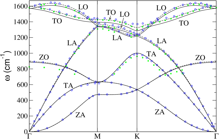
Figure 1: Ab initio phonon dispersion relation of graphene. Dashed line: LDA calculation, solid line: GGA calculation. We compare with LDA calculations by Dubay and Kresse [6] (circles) and GGA calculations by Maultzsch et al. [13] (asterisks).

The major breakthrough in the exact determination of the graphite-dispersion relation were the first ab-initio calculations by Kresse et al. [7] and Pavone et al. [9]. The calculations were done in the framework of DFT, employing the local-density approximation (LDA) to the exchange-correlation with a plane-wave expansion of the wavefunctions and using pseudo-potentials for the core-electrons. These calculations introduced considerable qualitative changes in the behavior of the high-frequency branches as compared to earlier force-constant fits. In particular, these calculations established a crossing of the longitudinal and transverse optical branches along the $\Gamma-K$ as well as the $\Gamma-M$ direction (see Fig. 1 below). Since then, improvements in the computer codes, the use of better pseudo-potentials and higher convergence-parameters have only led to small changes in the dispersion relations obtained by codes using plane-wave expansion and pseudopotentials. Slight variations mainly occur in the frequencies of the optical branches. Very recently, Maultzsch et al. presented ab-initio calculations [13] that are apparently in better agreement with experimental data. There are two sources of difference: the use of the generalized-gradient approximation (GGA) to the exchange-correlation functional and the use of a localized-orbital basis set.

In order to demonstrate the high degree of convergence of the theoretical calculations and in order to disentangle the influence of the exchange-correlation functional from the influence of the basis-set on the high-frequency modes, we have performed calculations both with the LDA and the GGA functional using a plane wave expansion. The only parameter that controls the basis set is the energy cutoff. Therefore, full convergence of the phonon frequency with respect to the basis set can be easily tested by increasing the energy cutoff.

The calculations have been performed with the code ABINIT [20, 21]. We use a periodic supercell with a distance of 10 a.u. between neighboring graphene-sheets. We checked that at this distance, the inter-layer interaction has virtually no effect on the phonon frequencies. (Calculations on bulk graphite are presented at the end of this section for completeness. Even there, the inter-plane interaction is so weak that it is only the branches with frequencies lower than 400 cm^-1 that are visibly affected). The dynamical matrix is calculated with DFPT [18]. For the LDA functional we use the Teter parameterization [22] and for the GGA functional the parameterization of Perdew, Burke, and Ernzerhof [23]. Core electrons are described by Troullier-Martins (TM) pseudopotentials [24]. For both LDA and GGA, an energy cutoff at 40 Ha. is used. The first Brillouin zone is sampled with a 20x20x2 Monkhorst-Pack grid. We employ a 0.004 a.u. Fermi-Dirac smearing of the occupation around the Fermi level. The phonon frequencies are converged to within 5 cm^-1 with respect to variation of the energy cutoff and variation of k-point sampling. The influence of the smearing parameter is negligible. The dynamical-matrix, which is the Fourier-transform of the real-space force constants, is calculated on a two-dimensional 18x18 Monkhorst-Pack grid in the reciprocal space of the phonon wave-vector ${\bf q}$. From this, the dynamical matrix at any ${\bf q}$ is obtained by interpolation. (We checked the quality of this interpolation by computing phonons for some ${\bf q}$-vectors not contained in the grid and comparing with the interpolated values).

The results of the calculation for the graphene sheet are presented in Fig. 1. We compare with the LDA calculations of Dubay and Kresse [6] who used the Vienna ab-initio simulation package (VASP) [25] with the projector augmented-wave (PAW) method [26] for the electron ion interaction. Also shown are the GGA results of Maultzsch et al. who used the SIESTA package [27] which also employs pseudopotentials for the core electron but uses a localized-orbital basis for the valence electrons. In contrast to plane-waves there is no easy way to check the convergence for a localized-orbital basis. Indeed, the converged value should be the one obtained with the plane-wave basis set. Any difference can be adscribed exclusively to the use of a localized basis set.

Before we analyze the differences between the different calculations, we outline the features common in all ab-initio calculations of graphite and graphene [7, 9, 17, 6, 14, 15, 13, 16]: The phonon dispersion relation of the graphene sheet comprises three acoustic (A) branches and three optical (O) branches. The modes affiliated with out-of-plane (Z) atomic motion are considerably softer than the in-plane longitudinal (L) and transverse (T) modes. While the TA and LA modes display the normal linear dispersion around the $\Gamma$-point, the ZA mode shows a $q^{2}$ energy dispersion which is explained in Ref. [1] as a consequence of the $D_{6h}$ point-group symmetry of graphene. Another consequence of the symmetry are the linear crossings of the ZA/ZO and the LA/LO modes at the K-point. These correspond to conical intersections in the two-dimensional parameter (${\bf q}$) space of the first Brillouin zone. Similarly, the electronic band structure of graphene displays a linear crossing at the K-point which marks the Fermi energy and is responsible for the semi-metallic behavior of graphene.

For a meaningful comparison of phonon frequencies obtained by different calculations (using different pseudo-potentials, basis-sets, parameterizations of the exchange-correlation functional), each calculation should be performed at the respective optimized lattice constant. For the discussion of the detailed differences between the calculations, we present in table 1 the frequencies at the high-symmetry points along with the respective optimized lattice constants. First, we compare our LDA calculation with the LDA calculation of Dubay and Kresse [6]. While we obtain a lattice constant of 2.449 Å, they obtain slightly different values (depending on whether they use a soft or a hard PAW). Nevertheless, the results for the phonon frequencies at $\Gamma$ and M are almost identical with their hard PAW results and only display minor differences ($\leq 1\%$) from their soft PAW results. Apparently, small errors in the pseudopotential that lead to small changes in the lattice constant are canceled in the phonon-calculation which samples the parabolic slope of the energy-hypersurface around the equilibrium position (at equilibrium lattice constant). This hypothesis was confirmed by test-calculations with other pseudo-potentials; e.g., a calculation with a Goedeker-Teter-Hutter potential [28] at an energy cutoff of 100 Ha., yielded a lattice constant of 2.442 a.u. and $\Gamma$-point frequencies of 903 and 1593 cm^-1 (compared with the 893 and 1597 cm^-1 of the TM pseudopotential). In contrast, if we perform a calculation with the Troullier-Martins pseudopotential at a lattice constant which is slightly (0.4%) enhanced with respect to the optimized value, we obtain the frequencies listed in table 2. These frequencies deviate by up to 2% from the calculation at the optimized lattice constant. We conclude that DFT-LDA calculations using plane-waves and performed at the respective optimized lattice constant can be considered well converged. Some differences remain only for the TO mode around the K-point which seems to be most susceptible to variations of the pseudopotential/PAW parameterizations. Besides that, all recent LDA calculations agree very well with each other.

We quote four significant figures for the calculated lattice constant because that is the order of convergence that can be achieved within the calculations. Changes in the last digit lead to noticeable (1%) changes in the phonon frequencies. However, it should be noted that the overall accuracy in comparison with experimental lattice constants is much lower for two reasons: (i) DFT in the LDA or GGA is an approximation to the exact $n$-electron problem. (ii) Temperature effects are neglected in the calculations, i.e., the calculations are performed for a fictitious classical system at zero temperature.

The widely accepted value for the lattice constant of graphite at room temperature is $a_{RT}=2.462$ Å [29, 30]. Scaling to zero temperature according to the thermal expansion data of Bailey and Yates [32] yields $a^{\prime}_{0K}=2.455$Å. However, comparing this value to the ab-initio value is, strictly speaking, not correct because the ab-initio value neglects the anharmonic effect of the zero-point vibrations. Instead, the ab-initio value should better be compared to the “unrenormalized” lattice constant at zero temperature, i.e. to the value obtained by linearly extrapolating the temperature dependence of the lattice constant at high temperature to zero temperature (see Fig. 3 of Ref. [31]). This “unrenormalized” value corresponds to atoms in fixed positions, not subject to either thermal or zero-point vibrations. With the linear expansion coefficient $\left.\alpha\right|_{T=270K}=\left.\frac{1}{a}\frac{da}{dT}\right|_{T=270K}=1.27^{-5}K^{-1}$ of Ref. [32], we obtain $a_{0K}=2.452$Å. This value is between the LDA value $a=2.449$Å and the GGA value $a=2.457$Å in agreement with the general trend that LDA underestimates and GGA overestimates the bond-length. We note that another value for the lattice constant that is sometimes quoted in the literature is the value of Baskin and Meyer [33]: $a_{RT}=2.4589\pm 0.0005$Å with a change less than 0.0005 Å as the specimen is cooled down to 78 K.

We turn now to the comparison of our LDA and GGA calculations. Following our statement above, we present calculations at the respective optimized lattice constants. Fig. 1 and Tab. 1 demonstrate very good agreement for the acoustic and the ZO modes. The deviation hardly ever reaches 1% of the phonon frequency. For the LO and TO modes, the GGA frequencies are softer by about 2% than the LDA values. Particularly sensitive is the K-point where the softening of GGA versus LDA reaches almost 3% (37 cm^-1). However, in order to put this effect of $v_{xc}$ into the right perspective, we note that the choice of the pseudo-potential (soft PAW versus Troullier-Martins) within the LDA approximation has a similarly big effect on the TO mode at K as shown above. Contrary to what is stated in Ref. [13], the deviations at the K-point do not arise from a neglect of the long-range character of the dynamical matrix which is properly taken into account in the supercell-approach (see also Ref. [6] where the real space force constants are explicitly listed up to 20th-nearest-neighbor interaction). Compared to the experimental phonon-frequencies at the $\Gamma$-point which can be determined with high accuracy by Raman-spectroscopy [34, 35, 36, 37], the GGA yields a slight underestimation of the LO/TO mode while the LDA yields a slight overestimation. For the ZO mode, both LDA and GGA overestimate the experimental value by 4% and 3%, respectively.

Fig. 1 also displays the recent GGA calculation by Maultzsch et al. [13]. In general, the agreement is very good with two exceptions: i.) In our calculation the TO mode is about 2% softer. ii.) The localized-basis calculation yields at $\Gamma$ a ZO frequency of 825 cm^-1 which is considerably smaller than the Raman value of 868^-1. The differences are entirely due to the choice of the basis-set.

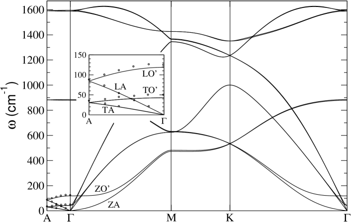
Figure 2: Ab initio (LDA) phonon dispersion relation of bulk-graphite. In the inset, an enlargement of the low-frequency phonons along the line $\Gamma$-A is shown. Symbols denote the neutron-scattering data of Nicklow et al. [38].

So far, we have only dealt with the single graphene sheet. In Fig. 2, we present a calculation of the dispersion relation of bulk graphite. The calculation is done with DFT-LDA using a 16x16x6 Monkhorst-Pack sampling of the first Brillouin zone. The unit-cell of graphite (ABA stacking) contains 4 atoms which give rise to 12 different phonon branches. However, as stated above, for frequencies higher than 400 cm^-1, the phonon branches are almost doubly degenerate since the inter-sheet interaction is very week. The degeneracy is lifted because in one case, equivalent atoms on neighboring sheets are oscillating in phase, while in the other case they are oscillating with a phase difference of $\pi$. This gives rise to small frequency differences of, in general, less than 10 cm^-1. E.g., the calculated frequency difference between the IR active $E_{1u}$ mode and the Raman active $E_{2g}$ mode at $\Gamma$ is 5 cm^-1 in perfect agreement with experiment (see table 1). Since the branches are almost degenerate, the comparison with experimental data can be done for phonon calculations of the graphene sheet only.

Only the phonon branches below 400 cm^-1 deviate noticeably from the branches of the sheet. They split into acoustic branches that approach 0 frequency for ${\bf q}\rightarrow 0$ (corresponding to in-phase oscillation of equivalent atoms of neighboring sheets) and “optical” modes that approach a finite value (corresponding to a phase-difference of $\pi$ in the oscillation of neighboring sheets). The optimized lattice constant is 2.449 Å as for the graphene sheet. As an optimized inter-layer distance we obtain $l=3.30$ Å which is only slightly lower than the experimental value of $l=3.34$ Å (measured at a temperature of 4.2 K [33]). This agreement is somewhat surprising. The inter-layer distance is so large that the chemical binding between neighboring-sheets (due to overlap of $\pi$-electron orbitals) is assumed to be weak. Van-der-Waals forces are expected to play a prominent role (up to the point that occasionally the term ”Van-der-Waals-binding” is used for the force that holds the graphite-sheets together). The Van-der-Waals interaction is, however, not properly described, neither in the LDA nor the GGA. (With GGA, we obtain an optimized lattice constant of 2.456 Å and a considerably overestimated inter-layer distance $l=3.90$ Å). The good agreement of experimental and LDA theoretical inter-sheet distance may therefore seem fortuitous. However, the detailed comparison of the low-frequency inter-layer modes with neutron-scattering data [38] demonstrate that also the total-energy curve around the equilibrium distance is reproduced with moderately good accuracy in the LDA. This was already seen in the calculation of Pavone et al. [9] and may be interpreted as an indication that at the inter-layer distance, the chemical binding still dominates over the Van-der-Waals force and only at larger inter-sheet distance the Van-der-Waals force will eventually be dominant. A more accurate description of the low-frequency modes will be an important test for the design of new functionals.

3 Experimental data

In this section we give a summary of the available experimental data for the phonon-dispersion relation of graphite. The data-points obtained by different experimental methods are collected in Fig. 3 and compared to our LDA and GGA calculations presented in the previous section.

Inelastic neutron-scattering is frequently used to obtain detailed information about the phonon-dispersion relation of crystalline samples. Since it is very difficult to obtain large high-quality samples of graphite, the available data [39, 38] is limited to the low-frequency ZA and LA branches (and the corresponding low frequency optical modes ZO’, TO’, and LO’). The significance of the agreement of theory and experiment for these branches has been discussed in the previous section.

High-resolution electron energy loss spectroscopy (HREELS) on graphite and thin graphite-films [40, 10, 11, 12, 16] has probed the high-symmetry directions $\Gamma$-K and $\Gamma$-M. The measurements (data-points marked by squares in Fig. 3) are consistent with each other and are in good agreement with the calculations, taking the scattering of the data points as a measure of the error bar. However, one apparent discrepancy persists for the TA mode (also called shear mode) around the M-point [6] where the EELS data converges towards 800 cm^-1 whereas the theory predicts 626 cm^-1 using LDA or 634 cm^-1 using GGA. (The difference between calculations is much smaller than the difference between theory and experiment). The HREELS selection rules actually state that this mode should be unobservable along the $\Gamma$-M direction owing to the reflection symmetry [41, 16]. Indeed, this branch was only observed in one experiment [10] on bulk graphite and was not observed for experiments on thin-films [16]. The appearance of this branch (and the discrepancy with respect to theory) may therefore tentatively be explained as a consequence of limited crystalline quality with the possible admixture of micro-crystallites of different orientation. Therefore, it should not be used to fit force-field parameters (see section 4 below). Instead, we will fit the parameters to the first-principles calculations where no crossing between the TA and ZA mode is present in the $\Gamma-M$ direction.

Raman-spectroscopy measures the phonon frequencies through the shift in the wave-length of inelastically scattered photons. In first-order Raman-scattering (one-phonon emission or absorption), only phonon-frequencies at the $\Gamma$-point can be detected, since the photons carry only vanishing momentum compared to the scale of phonon momenta. The selection rules of Raman-scattering, evaluated for the D_6h point-group of graphite pose a further restriction. The observable high-frequency mode [34, 35, 36, 37] is the $E_{2g}$ mode at 1587 cm^-1.

Infrared absorption spectroscopy yields a value of 1587-1590 cm^-1 for the E_1u mode and 868-869 cm^-1 for the A_2u mode at $\Gamma$ [34, 54].

In addition to the peaks due to symmetry allowed scattering-processes, Raman spectra frequently display additional features such as the disorder-induced $D$-band around 1350 cm^-1 (for laser excitation at about 2.41 eV). This feature is strongly dispersive with the laser energy and is explained as a $k$-selective resonance process [42, 43, 44]. A very elegant model is the double-resonant Raman effect proposed by Thomsen and Reich [45]. One possible scenario is a vertical resonant excitation of an electron with momentum ${\bf k}$ close to the K-point, followed by an inelastic transition to another excited state with momentum ${\bf k}+{\bf q}$ under emission or absorption of a phonon, elastic backscattering to the original ${\bf k}$ mediated by a defect, and de-excitation to the ground state by emitting a photon of different energy. The model was extended by Saito et al.[46, 3] to all branches of the phonon dispersion relation and was used to evaluate the data of earlier Raman experiments [43, 47, 48, 49, 50, 51, 52, 53]. The results are depicted in Fig. 3 by asterisks. The values close to $\Gamma$ are in fairly good agreement with the HREELS data and the ab-initio calculations. In particular, the values of the LO-branch coincide very well. A strong deviation of the double-resonant Raman data from the calculations can be observed at the $K$-point, in particular for the TO-mode. In the calculations, this mode is very sensitive to the convergence parameters and to the lattice constant (see tables 1 and 2). It may therefore not come as a surprise that the presence of defects which is an essential ingredient of the double-resonance Raman effect also yields a particularly strong modification of phonon frequencies for this branch at the $K$-point. The presence of defects may also explain the strong deviation of the double-resonant Raman data from both EELS-data and calculations along the ZO-branch.

Using inelastic x-ray scattering, Maultzsch et al. [13] have measured with high accuracy the high-frequency phonon branches. The LO and TO branches along $\Gamma$-M and $\Gamma$-K are in good agreement with the different HREELS measurements and are in almost perfect agreement with the GGA-calculation. The most important achievement is, however, that they experimentally established the dispersion relation along the line M - K. Also along this line, the agreement with ab-initio calculations is quite good even though not as good as along the other direction. Our calculations confirm the statement of Ref. [13] that GGA yields a slightly better agreement than LDA. Contrary to their calculation, however, we do not have to scale our theoretical results down by 1% in order to obtain the good agreement. This is because, we are using a fully converged plane wave basis set instead of a localized basis set. The remaining differences between theory and experiment may be due to small deviations from the high-symmetry lines in the experiment. At the same time, we recall that the GGA is still a very drastic approximation to the unknown “exact” exchange-correlation functional. Some of the remaining discrepancies could possibly be corrected by using “better” (as yet unknown) exchange-correlation functionals.

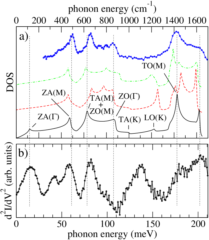
Figure 4: a) Vibrational density of states (vDOS) of graphite. Solid line: ab-initio calculation (LDA); dashed-line: 4NNFC model [1]; dash-dotted line: model of Aizawa et al. [11]; solid line with symbols: neutron-scattering on powdered sample [55]. Note that the model calculations are for the graphene-sheet such that the peak around 122 cm^-1 which is due to inter-plane coupling is missing. b) second derivative of the I-V curve for inelastic scanning-tunneling spectroscopy [15] of a graphite-surface. For the assignments of modes, see Fig. 1.

So far, limited crystal quality has prevented the measurement of the full dispersion relation by means of neutron scattering. However, neutron scattering on a powdered graphite sample has yielded the generalized vibrational density of states (GvDOS) [55] of graphite. The term ”generalized” means that each phonon mode is weighted by the cross section for its excitation. The data is shown in Figure 4 a). We compare with the ab-initio vDOS [15] (calculated with LDA) and the vDOS obtained from the model parameterization of Aizawa et al. [11] and from the 4NNFC approach of Ref. [5] (see next section about the details of the models). The most pronounced peaks arise from the high symmetry points as denoted in the figure and are in very good agreement with the ab-initio vDOS. The experimental DOS seems to confirm that the TA mode around the $M$-point has a frequency lower than 650 cm^-1 which is in close agreement to the ab-initio vDOS where the maxima arising from the TA($M$) and the ZO($M$) modes form one peak.

It can also be seen that the K-point phonons only contribute weak peaks to the ab-initio vDOS between 900 and 1300 cm^-1 which are not resolved in the experimental vDOS. In contrast, the two model-calculations display a strong peak around 1200-1250 cm^-1 which arises from an incorrectly described LA mode along the line $K-M$.

Recently, the vibrational density of states of graphite has also been measured by inelastic scanning tunneling spectroscopy (STS) [15]. The effect of phonon-scattering yields clear peaks at the corresponding energies in the second derivative of the I-V curve (Fig. 4 b). Not all features of the vDOS are resolved and additional inelastic scattering effects like plasmon excitations seem to occur. However, the agreement with the vibrational density of states is quite striking indicating that most (if not all) phonon modes can be excited in STS.

In conclusion, the different experimental methods are in good agreement with each other and yield a fairly complete picture of the phonon dispersion relation and the vibrational density of states. The agreement with the theoretical curves, in particular with the GGA calculation is very good. Some small differences remain: On the experimental side, limited crystal quality and the difficulty to perfectly align the crystal samples yield some scattering of the data points. More important however may be the role of temperature. While most experiments are performed at room temperature, the calculations are performed in the harmonic approximation for a classical crystal at zero temperature. While ab-initio calculations for the temperature dependence of phonons in graphite are still missing, recent calculations [56] for MgB₂ have demonstrated that the high symmetry phonons at room temperature are softer by about 1% than the phonons at zero temperature. Assuming a similar temperature dependence for graphite, the effect of temperature is of similar magnitude as the difference between LDA and GGA. The small differences between the different calculations should therefore be taken with caution whenever the quality of the approximations are assessed by comparison with experimental data.

4 Force constant approaches

We have shown in the previous sections that the major goal of an accurate calculation of graphite-phonons in agreement with experiment has been achieved. Nevertheless, for investigation of carbon nanostructures (in particular, nanotubes) it is often desirable to have a force-constant parametrization for fast - yet reliable - calculations. We review in this section the two main approaches found in the literature on graphite phonons: the valence-force-field (VFF) model and the direct parametrization of the diagonal real-space force-constants up to 4th-nearest-neighbor (4NNFC approach). We also give a new parametrization of both models fitted to our first-principles calculations.

The general form of the force-constant matrix for the interaction of an atom with its nth-nearest neighbor in the graphene sheet is

$$C_{n}=\left(\begin{array}[]{ccc}\phi^{l}_{n}&\xi_{n}&0\\ -\xi_{n}&\phi^{ti}_{n}&0\\ 0&0&\phi^{to}_{n}\\ \end{array}\right).$$ (4)

The coordinate system is chosen such that $x$ is the longitudinal coordinate (along the line connecting the two atoms), $y$ the transverse in-plane coordinate, and $z$ the coordinate perpendicular to the plane. The block-diagonal structure of the matrix reflects the fact that in-plane and out-of-plane vibrations are completely decoupled. In addition, $\xi_{1}=\xi_{3}=0$, due to the hexagonal-structure of graphene, i.e. displacing an atom towards its first/third nearest neighbor will not induce a transverse force on this atom. Up to 4th-nearest neighbor, there are thus 14 free parameters to determine.

The 4NNFC approach (see, e.g., Ref. [1]) makes the additional simplifying assumption that off-diagonal elements can be neglected, i.e. $\xi_{2}=\xi_{4}=0$. The force constant matrix describing the interaction between an atom and its nth-nearest neighbor has then the form

$$C_{n}=\left(\begin{array}[]{ccc}\phi^{l}_{n}&0&0\\ 0&\phi^{ti}_{n}&0\\ 0&0&\phi^{to}_{n}\\ \end{array}\right).$$ (5)

This means that a longitudinal displacement of an atom could only induce a force in longitudinal direction towards its nth neighbor, and a transverse displacement could induce only a transverse force. This assumption reduces the number of free parameters to 12.

The valence-force-field model determines the parameters of the matrix in Eq. 4 through the introduction of “spring constants” that determine the change in potential energy upon different deformations. The spring constants reflect the fact that a sp² bonded system tries to locally preserve its planar geometry and 120 degree bond angles. Aizawa et al [11], have introduced a set of 5 parameters, $\alpha_{1},\alpha_{2},\gamma_{1},\gamma_{2},$ and $\delta$. The parameters $\alpha_{1}$ and $\alpha_{2}$ are spring constants corresponding to bond-stretching, $\gamma_{1}$ is an in-plane and $\gamma_{2}$ an out-of-plane bond-bending spring constant, describing how the force changes as the in-plane and out-of-plane component of the bond-angle changes. In addition, the constant $\delta$ describes the restoring force upon twisting a bond.

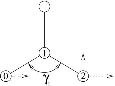
Figure 5: Illustration of the in-plane bending spring constant $\gamma_{1}$.

For a good introduction to the approach, we refer the reader to the appendix of Ref.[11]. Here, we just show as one example in figure 5 the effect of the force-constant $\gamma_{1}$. The potential energy corresponding to the in-plane angle bending is

$$\frac{\gamma_{1}}{2}\left[\left[\frac{({\bf u}_{0}-{\bf u}_{1})\times{\bf r}_{10}}{|{\bf r}_{10}|^{2}}\right]_{z}-\left[\frac{({\bf u}_{2}-{\bf u}_{1})\times{\bf r}_{12}}{|{\bf r}_{12}|^{2}}\right]_{z}\right]^{2},$$ (6)

where ${\bf u}_{i}$ indicates the displacement vector of atom $i$, ${\bf r}_{ij}$ is the relative mean position of atom $i$ from atom $j$, and the subscript $z$ means the component perpendicular to the surface.

Evaluating the forces that arise from the potential energy terms, the force-constant matrices for up to 4th-neighbor interaction take on the form

$$C_{1} = \left(\begin{array}[]{ccc}\alpha_{1}&0&0\\ 0&\frac{9}{2d^{2}}\gamma_{1}&0\\ 0&0&\frac{18}{d^{2}}\gamma_{2}\\ \end{array}\right),$$ (10)

$$C_{2} = \left(\begin{array}[]{ccc}\alpha_{2}+\frac{3}{4d^{2}}\gamma_{1}&\frac{3\sqrt{3}}{4d^{2}}\gamma_{1}&0\\ -\frac{3\sqrt{3}}{4d^{2}}\gamma_{1}&-\frac{9}{4d^{2}}\gamma_{1}&0\\ 0&0&-\frac{3}{a^{2}}\gamma_{2}+\frac{1}{d^{2}}\delta\\ \end{array}\right),$$ (14)

$$C_{3} = \left(\begin{array}[]{ccc}0&0&0\\ 0&0&0\\ 0&0&\frac{2}{d^{2}}\delta\\ \end{array}\right),$$ (18)

$$C_{4} = \left(\begin{array}[]{ccc}0&0&0\\ 0&0&0\\ 0&0&-\frac{1}{d^{2}}\delta\\ \end{array}\right).$$ (22)

The constant $d=d_{C-C}$ denotes the bond-length of graphite. In contrast to the 4NNFC parametrization, the diagonal in-plane terms in the 3rd and 4th nearest neighbor interaction are zero. On the other hand, the 2nd nearest-neighbor interaction has a non-diagonal term. As illustrated in Fig. 5, the force acting on atom 3 upon longitudinal displacement of atom 1 (keeping atom 2 fixed) has a longitudinal and transverse component. This is a consequence of the angular spring constant $\gamma_{1}$ that tries to preserve the 120 degree bonding. The appearence of the off-diagonal term in the VFF-model is the reason why this model with only 5 parameters can yield a fit of similar quality as the 4NNFC parametrization with 12 parameters (see Fig. 7 below). An early VFF-model [57, 58] in terms of only 3 parameters for the intra-sheet forces gave a good fit of the slope of the acoustic modes (which in turn determine the specific heat) but cannot properly describe the dispersion of the high-frequency modes.

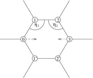
Figure 6: Illustration of third-nearest neighbor interaction. Upon displacement of atom 0 to the right and keeping all other atom fixed, atom 3 at the opposite corner of the hexagon experiences a force to the left.

An ab-initio calculation of the real-space force-constant matrices has confirmed the appearence of pronounced off-diagonal terms [6]. The interpretation of force-constants in terms of the VFF model is very instructive but limited to near neighbor interactions. The ab-initio calculations have, in contrast, demonstrated the long-range character of the dynamical matrix [6]. Possible extensions of the VFF-model would have to take into account the effects of the complex electronic rearrangement upon atomic displacement. E.g., the longitudinal force-constant $\phi^{l}_{3}$ for the third-nearest neighbor interaction is zero in the VFF model but turns out to be negative in the ab-initio calculations [6]. This is illustrated in Fig. 6. As atom 0 is pushed to the right (while atoms 1,1’,2,and 2’ are kept at fixed position), atom 3 experiences a force to the left. A similar behavior can be observed for the benzene ring. A possible interpretation is that the change of the angle $\eta_{1}$ (coming along with a small admixture of sp¹ and sp³ hybridizations to the sp² bonding of atom 1) induces a change in of the bond between atom 1 and 2. This change, in turn, imposes the same hybridization admixture to atom 2 and thereby tries to keep the angle $\eta_{2}=\eta_{1}$. The (in-plane) third-nearest neighbor interaction could thus be expressed in a potential-energy term of the form $~{}\frac{1}{2}c(\eta_{2}-\eta_{1})^{2}$. However, instead of adding additional degrees of complexity to the VFF-model, it is easier to fit the force-constants up to nth-nearest-neighbor directly.

We have fitted the five parameters of the VFF model and the 12 parameters of the 4NNFC model to our GGA-calculation (see Fig. 1). Furthermore, we have performed a fit with 13 parameters, where, in addition to the 4NNFC parameters, we allow for a non-zero off-diagonal parameter $\xi_{2}$ for the 2nd-nearest neighbor interaction. In table 3, we list the obtained parameters and compare with the parameterizations available in the literature. The resulting dispersion relations are displayed in Fig. 7. In all cases, we compare with our GGA-calculation which represents very well the bulk of the data-points as was demonstrated in Fig. 3. The fit parameters were obtained by minimizing

$$\chi^{2}=\sum_{n=1}^{N}\sum_{i=1}^{6}\left(\omega_{i,n}^{\mbox{model}}-\omega_{i,n}^{\mbox{GGA}}\right)^{2}$$ (24)

for the 6 phonon branches on $N=237$ $q$-points along the high-symmetry directions of the first Brillouin zone. The resulting standard-deviation $\sigma=\sqrt{\chi^{2}/N/6}$ may serve as a measure of the quality of the fit and is also listed in table 3.

The 4NNFC parameterizations (Fig. 7 a and b) and the VFF parameterizations (Fig. 7 e) that are available in the literature reproduce very well the slope of the acoustic branches. However, large deviations occur for the high-frequency modes, in particular at the edge of the first Brillouin zone. E.g., the fit in Fig. 7 b) fails completely to reproduce the crossings of the LO and TO branches along the lines $\Gamma-M$ and $\Gamma-K$, and the fits in a) and e) reproduce it only along the line $\Gamma$-K. Our fit of the 4NNFC model (Fig. 7 c) yields a major improvement (with a mean deviation $\sigma=15.4$ cm^-1), however still does not reproduce the LO-TO crossing along $\Gamma-M$. This is only achieved, if we include the off-diagonal term $\xi_{2}$ in the model. This gives only a slight improvement in terms of the standard deviation ($\sigma=13.5$ cm^-1) but leads to a qualitatively correct ordering of the high-frequency modes also along the line $M-K$. Clearly, for a very high-accuracy fit, a fourth-nearest-neighbor approach is not enough. In particular, the TO phonon at the K-point is very sensitive to the parametrization and can only be accurately described if the long-range character of the dynamical matrix is properly taken into account [13]. However, our fit has an average deviation of only 1% from the GGA-curve and a maximum deviation (at $K$) of 4%. For many practical calculations this accuracy is more than sufficient and we therefore expect, that our fit to the ab-initio calculations may be of some help in the future. Even the 4NNFC fit without the diagonal term should be sufficient for many applications, provided that the details of the high-frequency phonon branches along $M-K$ are not important.

We have also fitted the VFF-model to the GGA calculation (Fig. 7 f). Since this model contains only five parameters, it cannot compete in accuracy with the 4NNFC. In particular, since we fit for phonons of the whole Brillouin-zone, the slope of the acoustic modes around $\Gamma$ deviates from the correct value.

Our comparison of force-constant models shows that the parameterizations in the literature display some strong deviations from the presumably correct dispersion relation. Nevertheless, in many applications of these models, these deviations are not of major concern. E.g. for the calculation of the sound-velocity and the elastic constants, only the slope of the acoustic branches at $\Gamma$ needs to be described properly. Another example is the description of Raman spectroscopy in carbon nanotubes. The Raman active modes of the tube can be mapped onto phonon modes of graphene with a momentum close to zero for large diameter tubes. Therefore, for first order Raman scattering, only the dispersion close to $\Gamma$ needs to be well reproduced by the model. This is indeed fulfilled by the available force-constant fits, as Fig. 7 demonstrates. However, for applications where the whole Brillouin-zone is sampled (e.g. for the interpretation of double-resonant Raman spectra) the present fit provides a considerably more accurate description.

5 Conclusion

In the present work we have reviewed the experimental and theoretical studies of the phonon dispersion in graphene and graphite. We have provided a detailed discussion of the different approximations used in the first principles calculations. In particular we have shown the effect of the exchange-correlation potential $v_{xc}$ on the phonon-dispersion relation for a calculation with a fully converged plane-wave basis. The GGA yields phonons in the high-frequency region that are softer by about 2% than phonons calculated in the LDA. We have demonstrated that for a consistent comparison of different calculations (with different $v_{xc}$ or different pseudopotentials) it is mandatory to perform the calculation at the respective optimized lattice-constant. Under these conditions, recent LDA-calculations using plane waves give very similar results and can be considered fully converged (with some minor residual differences due to the employed pseudopotentials). In Fig. 3, where we have collected the available experimental data-points, obtained by different spectroscopy methods, we have shown that the ab-initio calculations reproduce very well the vast majority of the experimental data. The GGA yields a slightly better agreement for the high-frequency branches than the LDA.

Concerning force-constant models, we have fitted a fourth-nearest neighbor model to our GGA calculation and obtain very good agreement between the model and first-principles calculations. Minor discrepancies for the LO and TO branches (in particular close to the K-point) are related to the lack of long-range interactions in the model. This parametrization, in particular if the off-diagonal term for second-nearest neighbor interaction is taken into account, provides a coherent description of the first principles calculations and does not suffer from uncertainties related to different experimental techniques. We hope that the model will be of use for further calculations of phonons in carbon nanotubes and other nanostructures.

6 Acknowledgment

We acknowledge helpful communication with experimentalists: D. Farias, J. L. Sauvajol, J. Serrano, L. Vitali, and H. Yanagisawa and theorists: G. Kresse and M. Verstraete. The work was supported by the European Research and Training Network COMELCAN (Contract No. HPRN-CT-2000-00128) and the NANOQUANTA network of excellence (NOE 500198-2). The calculations were performed at the computing center of the DIPC and at the European Center for parallelization of Barcelona (CEPBA).

		Ref. [6]	Ref. [6]	this work	this work	Ref. [13]
$v_{xc}$		LDA	LDA	LDA	GGA	GGA	Experiment
pseudo-potential		soft PAW	hard PAW	TM	TM	TM
basis-expansion		plane-wave	plane-wave	plane-wave	plane-wave	local orbitals
opt. lattice constant		2.451 Å	2.447 Å	2.449 Å	2.457 Å	?	2.452e Å
$\Gamma$	ZO	890	896	893	884	825	868a
	LO/TO	1595	1597	1597	1569	1581	1582b,1587c
M	ZA	475	476	472	476
	TA	618	627	626	634
	ZO	636	641	637	640
	LA	1339	1347	1346	1338	1315	1290d
	LO	1380	1373	1368	1346	1350	1323d
	TO	1442	1434	1428	1396	1425	1390d
K	ZO/ZA	535		535	539
	TA	994		1002	1004
	LO/LA	1246		1238	1221	1220	1194d
	TO	1371		1326	1289	1300	1265d

Table 1: Comparison of most recent DFT-calculations of phonon frequencies (in cm^-1) at high-symmetry points in graphene. For the $\Gamma$-point we also list the experimental values obtained by infrared absorption and Raman scattering (^aRef. [34], ${}^{b}\omega(E_{2g})$, Refs. [34, 35, 36], ${}^{c}\omega(E_{1u})$, Refs. [34] and [37]). For the $M$ and $K$-points we list inelastic x-ray data of ^dRef. [13]. ^eThe experimental lattice constant is the “unrenormalized” zero temperature value (see text).

		$a_{opt.}$	$a_{exp.}$			$a_{opt.}$	$a_{exp.}$			$a_{opt.}$	$a_{exp.}$
$\Gamma$	ZO	893	894	$M$	LA	1346	1337	$K$	LO/LA	1238	1225
	LO/TO	1597	1575		LO	1368	1350		TO	1326	1298
					TO	1428	1404

Table 2: Comparison of high-frequency modes calculated with LDA at the optimized lattice constant ($a_{opt.}=2.449$ Å, as in Table 1) and at the lattice constant $a=2.458$ Å. The small (0.4%) change in the lattice constant affects strongly the high-frequency modes (up to 2% shift).

Force Constant Fits
	4NNFC	4NNFC	4NNFC	4NNFC
	diagonal	diagonal	diagonal	+ off-diag. coupling
	Ref. [5]	Ref. [3]	fit to GGA	fit to GGA
$\sigma$ (cm-1)	51.5	69.5	15.4	13.5
$\phi^{l}_{1}$ (104 dyn/cm)	36.50	40.37	39.87	40.98
$\phi^{l}_{1}$ (104 dyn/cm)	8.80	2.76	7.29	7.42
$\phi^{l}_{1}$ (104 dyn/cm)	3.00	0.05	-2.64	-3.32
$\phi^{l}_{1}$ (104 dyn/cm)	-1.92	1.31	0.10	0.65
$\phi^{ti}_{1}$ (104 dyn/cm)	24.50	25.18	17.28	14.50
$\phi^{ti}_{1}$ (104 dyn/cm)	-3.23	2.22	-4.61	-4.08
$\phi^{ti}_{1}$ (104 dyn/cm)	-5.25	-8.99	3.31	5.01
$\phi^{ti}_{1}$ (104 dyn/cm)	2.29	0.22	0.79	0.55
$\phi^{to}_{1}$ (104 dyn/cm)	9.82	9.40	9.89	9.89
$\phi^{to}_{1}$ (104 dyn/cm)	-0.40	-0.08	-0.82	-0.82
$\phi^{to}_{1}$ (104 dyn/cm)	0.15	-0.06	0.58	0.58
$\phi^{to}_{1}$ (104 dyn/cm)	-0.58	-0.63	-0.52	-0.52
$\xi_{2}$ (104 dyn/cm)	0	0	0	-0.91
Valence-Force-Field Fits
	Ref. [11]	Ref. [12]	fit to GGA
$\sigma$ (cm-1)	47.3	55.0	33.6
$\alpha_{1}$ (104 dyn/cm)	36.4	34.4	39.9
$\alpha_{2}$ (104 dyn/cm)	6.2	6.2	5.7
$\gamma_{1}$ (10-13 erg)	83.0	93.0	60.8
$\gamma_{2}$ (10-13 erg)	33.8	30.8	32.8
$\delta$ (10-13 erg)	31.7	41.7	34.6

Table 3: Force constant and valence-force-field parameterizations for graphene. Comparison of literature values with our fit to the GGA calculation. The standard deviation $\sigma$ is calculated for each parameterization with respect to the GGA calculation. The corresponding dispersion relations are shown in Fig. 7.

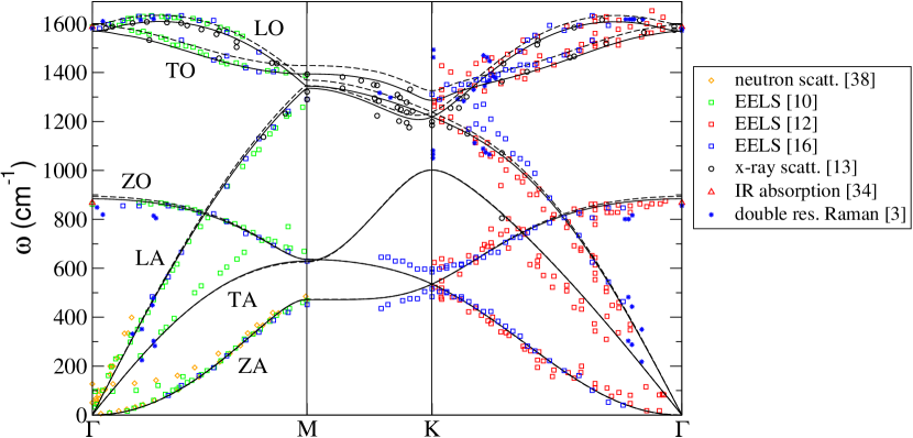
Figure 3: (Color online): Experimental data points for the phonon-dispersion relation of graphite. Diamonds: neutron scattering [38], squares: EELS [10, 12, 16], circles: x-ray scattering [13], triangles: IR absorption [34], asterisks: data of various double resonant Raman scattering experiments, collected in Ref. [3]. We compare with our ab-initio calculations: dashed line: LDA, solid line: GGA (as in Fig. 1).

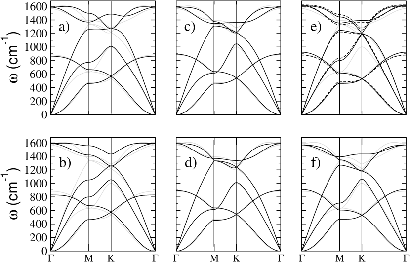
Figure 7: Comparison of 4NNFC and VFF fits (black lines) with the GGA calculation (grey line). The corresponding parameters are listed in Tab. 3. a) 4NNFC fit of Ref. [5], b) 4NNFC fit of Ref. [3] , c) Our 4NNFC fit to the GGA, d) Our 4NNFC fit to the GGA including off-diagonal term for the 2nd-nearest neighbor interaction, e) VFF fit of Ref. [11] (solid line) and Ref. [12] (dashed line), f) Our VFF fit to the GGA. Overall, the fits (c) and (d) clearly reproduce most of the features of the phonon-dispersion relation of graphene. Notable exceptions are the TO mode at $K$ and the missing overbending of the LO branch. These are related to the long-range nature of the dynamical matrix and can only be properly reproduced with fits that take into account the interaction of atoms more distant than fourth-nearest neighbor.

References

- [1] R. Saito, G. Dresselhaus, and M. S. Dresselhaus, Physical Properties of Carbon Nanotubes (Imperial College Press, London, 1998).
- [2] M. S. Dresselhaus, G. Dresselhaus, and Ph. Avouris (Eds.), Carbon nanotubes: synthesis, structure, properties, and applications (Springer-Verlag, Berlin Heidelberg, 2001).
- [3] A. Grüneis, R. Saito, T. Kimura, L. C. Cancado, M. A. Pimienta, A. Jorio, A. G. Souza Filho, G. Dresselhaus, and M. S. Dresselhaus, Phys. Rev. B 65, 155405 (2002).
- [4] R. A. Jishi and G. Dresselhaus, Phys. Rev. B 26, 4514 (1982).
- [5] R. A. Jishi, L. Venkataraman, M. S. Dresselhaus, and G. Dresselhaus, Chem. Phys. Lett. 209, 77 (1993).
- [6] O. Dubay and G. Kresse, Phys. Rev. B 67, 035401 (2003).
- [7] G. Kresse, J. Furthmüller, and J. Hafner, Europhys. Lett. 32, 729 (1995).
- [8] Y. Miyamoto, M. L. Cohen, and S. G. Louie, Phys. Rev. B 52, 14971 (1995).
- [9] P. Pavone, R. Bauer, K. Karch, O. Schütt, S. Vent, W. Windl, D. Strauch, S. Baroni, and S. de Gironcoli, Physica B 219 & 220, 439 (1996).
- [10] C. Oshima, T. Aizawa, R. Souda, Y. Ishizawa, Y. Sumiyoshi, Solid state Comm. 65, 1601 (1988).
- [11] T. Aizawa, R. Souda, S. Otani, Y. Ishizawa, and C. Oshima, Phys. Rev. B 42, 11469 (1990).
- [12] S. Siebentritt, R. Pues, K-H. Rieder, and A. M. Shikin, Phys. Rev. B 55, 7927 (1997).
- [13] J. Maultzsch, S. Reich, C. Thomsen, H. Requardth, and P. Ordejón, Phys. Rev. Lett. 92, 075501 (2004).
- [14] L. Wirtz, A. Rubio, R. Arenal de la Concha, and A. Loiseau, Phys. Rev. B 68, 045425 (2003).
- [15] L. Vitali, M. A. Schneider, K. Kern, L. Wirtz, and A. Rubio, Phys. Rev. B 69, 121414 (2004)
- [16] H. Yanagisawa, T. Tanaka, Y. Ishida, M. Matsue, E. Rokuta, S. Otani, and C. Oshima, submitted to SIA (2004).
- [17] D. Sánchez-Portal, E. Artacho, J. M. Soler, A. Rubio, and P. Ordejón, Phys. Rev. B 59, 12678 (1999).
- [18] S. Baroni, S. de Gironcoli, A. Dal Corso and P. Giannozzi, Rev. Mod. Phys. 73, 515 (2001);
- [19] X. Gonze, Phys. Rev. B 55, 10337 (1997).
- [20] The ABINIT code is a common project of the Université Catholique de Louvain, Corning Incorporated, and other contributors (URL http://www.abinit.org).
- [21] X. Gonze et al. Comp. Mat. Sci. 25, 478 (2002).
- [22] S. Goedecker, M. Teter, J. Huetter, Phys. Rev. B 54, 1703 (1996).
- [23] J. P. Perdew, K. Burke, and M. Ernzerhof, Phys. Rev. Lett. 77, 3865 (1996).
- [24] N. Troullier and J. L. Martins, Phys. Rev. B 64, 1993 (1991).
- [25] G. Kresse and J. Hafner, Phys. Rev. B 48, 13115 (1993).
- [26] P. E. Blöchl, Phys. Rev. B 50, 17953 (1994).
- [27] J. M. Soler et al., J. Phys. Condens. Matter 14, 2745 (2002).
- [28] S. Goedeker, M. Teter, and J. Hutter, Phys. Rev. B 54, 1703 (1996).
- [29] B. T. Kelly, Physics of Graphite, Applied Science, London, 1981.
- [30] M. S. Dresselhaus, G. Dresselhaus, K. Sugihara, I. L. Spain, and H. A. Goldberg, Graphite Fibers and Filaments, Springer, Heidelberg, 1988.
- [31] M. Cardona, in Electrons and Photons in Solids, A Volume in honour of Franco Bassani, Scuola Normale, Pisa. 2001, p. 25.
- [32] A. C. Bailey and B. Yates, J. Appl. Phys. 41, 5088 (1970).
- [33] Y. Baskin and L. Mayer, Phys. Rev. 100, 544 (1955).
- [34] R. J. Nemanich, G. Lucovsky, and S. A. Solin, Mater. Sci. Eng. 31, 157 (1977).
- [35] F. Touinstra and J. L. Koenig, J. Chem. Phys. 53, 1126 (1970).
- [36] L. J. Brillson. E. Burstein, A. A. Maradudin, and T. Stark, in The Physics of Semimetals and Narrow Gap Semiconductors, edited by D. L. Carter and R. T. Bate (Pergamon, Oxford, 1997), p. 187.
- [37] R. A. Friedel and G. C. Carlson, J. Phys. C 75, 1149 (1971).
- [38] R. Nicklow, N. Wakabayashi, and H. G. Smith, Phys. Rev. B 5, 4951 (1972).
- [39] G. Dolling and B. N. Brockhouse, Phys. Rev. 128, 1120 (1962).
- [40] J. L. Wilkes et al., J. Electron Spectrosc. Relat. Phenom. 44, 355 (1987).
- [41] H. Ibach and D. L. Mills, Electron Energy Loss Spectroscopy and Surface Vibrations, Academic, New York, 1982.
- [42] M. J. Matthews et al., Phys. Rev. B 59, R6585 (1999).
- [43] I. Pócsik et al., J. Non-Cryst. Solids 227-230, 1083 (1998).
- [44] A. C. Ferrari and J. Robertson, Phys. Rev. B 64, 075414 (2001).
- [45] C. Thomsen and S. Reich, Phys. Rev. Lett. 85, 5214 (2000).
- [46] R. Saito, A. Jorio, A.G. Souza Filho, G. Dresselhaus, M. S. Dresselhaus, and M. A. Pimenta, Phys. Rev. Lett. 88, 027401 (2002).
- [47] M. A. Pimenta et al., Braz. J. Phys. 30, 432 (2000).
- [48] P. H. Tan et al., Phys. Rev. B 64, 214301 (2001).
- [49] P. H. Tan et al., Phys. Rev. B 58, 5435 (1998).
- [50] Y. Kawashima et al., Phys. Rev. B 52, 10053 (1995).
- [51] Y. Kawashima et al., Phys. Rev. B 59, 62 (1999).
- [52] L. Alvarez et al., Chem. Phys. Lett. 320, 441 (2000).
- [53] P. H. Tan et al., Appl. Phys. Lett. 75, 1524 (1999).
- [54] U. Kuhlmann, H. Jantoljak, N. Pfänder, P. Bernier, C. Journet, and C. Thomasen, Chem. Phys. Lett. 294, 237 (1998).
- [55] S. Rols, Z. Benes, E. Anglaret, J. L. Sauvajol, P. Papanek, J. E. Fischer, G. Coddens, H. Schober, and A. J. Dianoux, Phys. Rev. Lett. 85, 5222 (2000).
- [56] M. Lazzeri, M. Calandra, and F. Mauri, Phys. Rev. B 68, 220509 (2003).
- [57] A. Yoshimori and Y. Kitano, J. Phys. Soc. Japan 2, 352 (1956).
- [58] J. A. Young, and J. U. Koppel, J. Chem. Phys. 42, 357 (1963).