Field-induced gap in ordered Heisenberg antiferromagnets

Abstract

Heisenberg antiferromagnets in a strong uniform magnetic field $H$ are expected to exhibit a gapless phase with a global O(2) symmetry. In many real magnets, a small energy gap is induced by additional interactions that can be viewed as a staggered transverse magnetic field $h=cH$, where $c$ is a small proportionality constant. We study the effects of such a perturbation, particularly for magnets with long-range order, by using several complimentary approaches: numerical diagonalizations of a model with long-range interactions, classical equations of motion, and scaling arguments. In an ordered state at zero temperature, the energy gap at first grows as $(cH)^{1/2}$ and then may dip to a smaller value, of order $(cH)^{2/3}$, at the quantum critical point separating the “gapless” phase from the gapped state with saturated magnetization. In one spatial dimension, the latter exponent changes to 4/5.

I Introduction

The investigation of quantum antiferromagnets in strong magnetic fields is currently a very active field of research. Several remarkable properties have been observed, such as the closing of the energy gap in spin-1 chainszheludev and spin ladderschaboussant and observations of magnetization plateaux in frustrated magnets.kageyama ; kodama While the broad features of these models can be explained in the framework of the Heisenberg model in a uniform magnetic field, a closer examination of experimental data reveals deviations from theoretically predicted behavior. In particular, the supposedly gapless phases actually possess small energy gaps, which can only be explained by the presence of anisotropic interactions.

For instance, Dender et al.D97 discovered that an applied magnetic field ${\bf H}$ induces in spin-1/2 Heisenberg chains a gap $\Delta\propto H^{0.65(3)}$. Oshikawa and AffleckO97 ascribed the gap to a staggered transverse field arising from the staggering of the $g$-tensor or of the Dzyaloshinskii-Moriya (DM) interaction. They suggested the effective Hamiltonian

$${\cal H}=\sum_{n}[J{\bf S}_{n}\cdot{\bf S}_{n+1}-HS_{n}^{z}-h\,(-1)^{n}S_{n}^{x}],$$ (1)

where $h\propto H$. The transverse field ${\bf h}$ creates a spin gap $\Delta\propto h^{2/3}\propto H^{2/3}$, in agreement with the experiment and density-matrix renormalization group (DMRG) calculations.L02 ; Zhao03

An extension of these results to higher dimension is still at a preliminary stage. Sato and OshikawaSato04 studied a model of interacting chains with a staggered field induced by the DM interactions and found that the gap scales as $\Delta\propto H^{1/2}$ in a weak field. The recent discoverykageyama of the Shastry–Sutherland antiferromagnet ${\rm SrCu_{2}(BO_{3})_{2}}$ calls for further studies in two dimensions. In particular, the presence of a staggered magnetization in the low-field NMR signal was ascribed to a staggering of the $g$-tensor and of the DM interaction.kodama2 The direct numerical investigation of the relevant microscopic models does not seem to be possible at the moment. Indeed, to get a reliable estimate of the small gap induced by anisotropic interactions requires to reach sizes such that the finite-size gaps, typically of order $J/N$ for $N$ sites, are much smaller than the physical gap. This is possible in 1D with the help of the DMRG algorithm, which by now routinely allows one to study systems with 200 sites or more, but not in 2D.

In this paper, we present the first systematic study of this problem in the context of the Lieb-Mattis model,LM62 wherein every spin of one sublattice is coupled equally to all spins of the other. This model is expected to provide a fair description of the long-wavelength properties of bipartite Heisenberg antiferromagnets with long-range Néel order in the ground state. Therefore it should be relevant for magnets in 2 and 3 dimensions.

We pay particular attention to the high-field regime where the uniform magnetization saturates. In the absence of a staggered field, the saturation occurs at a critical point $H=H_{c}$ separating a gapless ordered phase with a spontaneously broken rotational O(2) symmetry from a gapped phase with fully polarized spins. The behavior of the transverse-field spin gap near the critical field $H_{c}$ is an important problem in view of its relevance to a number of experimental systems. Unlike the weak-field regime, for which analytical results have been obtained, the saturation region has so far been studied only numerically.L02 ; Zhao03 Curiously, the numerical data reveal a nonmonotonic dependence $\Delta(H)$, with a pronounced minimum near the saturation field $H_{c}$. A similar effect was noticed earlier by Sakai and Shiba in their numerical analysis of spin-1 chains.Sakai94

II The Lieb–Mattis model

In this section, we concentrate on the Lieb-Mattis model describing a Heisenberg antiferromagnet on a bipartite lattice in which every spin of one sublattice is coupled through antiferromagnetic exchange to all sites of the other sublattice. Its Hamiltonian describes spins of length $S$ in a uniform magnetic field ${\bf H}=(0,0,H)$ and a staggered field ${\bf h}=(h,0,0)$ perpendicular to it:

$${\cal H} = (J/N)\sum_{\bf r\in A}\sum_{\bf r^{\prime}\in B}{\bf S}_{\bf r}\cdot{\bf S}_{\bf r^{\prime}}$$

$$-\sum_{\bf r\in A}({\bf H}+{\bf h})\cdot{\bf S}_{\bf r}-\sum_{\bf r\in B}({\bf H}-{\bf h})\cdot{\bf S}_{\bf r}$$

$$= (J/N)\,{\bf S}_{A}\cdot{\bf S}_{B}-H(S_{A}^{z}+S_{B}^{z})-h(S_{A}^{x}-S_{B}^{x}),$$

where ${\bf S}_{A}$ and ${\bf S}_{B}$ are the total spins of sublattices A and B. The exchange constant $J$ is normalized by the total number of sites $N$ to make the energy of the model an extensive quantity ${\mathcal{O}}(N)$. To reflect the induced origin of the staggered field ${\bf h}$, we will set $h=cH$, where the constant $c\ll 1$ is a property of the system.

In zero transverse field, the Hamiltonian (II) has an O(2) rotational symmetry and is readily diagonalized. The energy levels are expressed in terms of the total spins of the sublattices $S_{A}$ and $S_{B}$, the total spin $S_{\rm tot}$ and its projection $S_{\rm tot}^{z}$ on the direction of the uniform field ${\bf H}$:

$$E_{0} = (J/2N)S_{\rm tot}(S_{\rm tot}+1)-HS_{\rm tot}^{z}$$ (3)

$$- (J/2N)[S_{A}(S_{A}+1)+S_{B}(S_{B}+1)].$$

In the ground state the sublattices are fully polarized, $S_{A}=S_{B}=NS/2$, and the total angular momentum points along ${\bf H}$: $S_{\rm tot}^{z}=S_{\rm tot}$. Excitations reducing sublattice magnetizations have an energy gap ${\mathcal{O}}(JS)$. Below saturation, $H\leq H_{c}=JS$, low-energy excited states are obtained by changing the quantum numbers $S_{\rm tot}^{z}=S_{\rm tot}$ from their ground-state values. These excitations have energy ${\mathcal{O}}(JS/N)$ and form a continuum in the limit $N\to\infty$. The gapless excitations are caused by spontaneous breaking of the O(2) symmetry. Indeed, for $N\to\infty$ the sublattice spins ${\bf S}_{A}$ and ${\bf S}_{B}$ become classical vectors with well-defined directions in space (Fig. 1). In the absence of the transverse staggered field ${\bf h}$, the sublattice moments can be freely rotated about ${\bf H}$. The low-energy excitations thus correspond to a slow precession of ${\bf S}_{A}$ and ${\bf S}_{B}$ when the angle $\theta$ deviates slightly from the equilibrium value $\theta=\arcsin{(H/JS)}$.

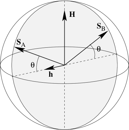
Figure 1: A classical ground state. The sublattice spins reside in the plane formed by the vectors ${\bf H}$ and ${\bf h}$.

Adding the transverse field ${\bf h}$ breaks the O(2) symmetry explicitly and violates conservation of both $S_{\rm tot}$ and $S_{\rm tot}^{z}$. Nonetheless, lengths of the sublattice spins $S_{A}$ and $S_{B}$ are still good quantum numbers. This fact greatly simplifies the numerical diagonalization of the Hamiltonian (II).

II.1 Exact diagonalizations

Because the ground state and all low-lying excitations of the model with ${\bf h}=0$ are in the sector $S_{A}=S_{B}=NS/2$, we will restrict our analysis of the gap to that sector. The size of this subspace for $N$ spins equals $(NS+1)^{2}$, which is smaller than the size of the total Hilbert space, $(2S+1)^{N}$. This enables us to treat systems with rather large numbers of spins. In the following, we present results for 2000 spins $S=1/2$, a size clearly beyond the scope of exact diagonalizations of other Heisenberg models without additional conserved quantities.

We first calculate the gap as a function of $h$ in the absence of a uniform field. The results are plotted in Fig.2. By fitting the data at low field $h\to 0$, we determined that the gap vanishes as $\Delta\sim\sqrt{JSh}$, precisely as found by Oshikawa and Affleck in the approximation of noninteracting magnons.O97 This result is most easily understood by computing the precession frequency of sublattice magnetizations at the classical level, as we do in the next section. The result of this calculation is plotted as a solid line in Fig. 2. An excellent agreement shows that size effects are already negligible for $N=2000$ (with the exception of a finite gap at $h=0$).

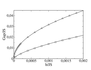
Figure 2: The spin gap $\Delta$ as a function of the transverse field $h$ for two values of the uniform field: $H=0$ (triangles) and $H=H_{c}=JS$ (squares) for $N=2000$. The curves are the results of the spin-wave analysis.

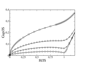
Figure 3: The spin gap as a function of $H$ at $h=cH$ for several value of the proportionality constant: $c=0.1$ (squares), 0.03 (triangles up), 0.01 (triangles down) and 0.0025 (circles). The gap has a local minimum for $c\leq 0.03$. Lines are the results of the spin-wave analysis.

Next we consider the case where the staggered field is proportional to the uniform field: $h=cH$. Typical results obtained for various values of $c$ are plotted in Fig. 3. As $H\to 0$, $\Delta\sim H^{1/2}$ with numerical precision. The behaviour at higher fields depends on the value of the proportionality constant $c$. If it is small enough, $c<0.03\pm 0.005$, the gap exhibits a local minimum close to—and slightly below—the saturation field. Such a dip has been observed previously in numerical studies of 1D models,Zhao03 but no explanation has been given so far. To get further insight, we have kept the uniform field at its saturation value $H_{c}=JS$ and calculated the gap as a function of $h$. The results are plotted in Fig.2. They are consistent with a power-law scaling $\Delta\propto h^{2/3}$. We will return to this phenomenon in the next section.

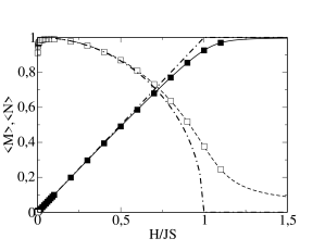
Figure 4: Uniform (filled squares) and staggered (open squares) magnetizations for $N=2000$ as a function of $H$ for $c=0.03$. Solid and dashed lines are results of the spin-wave analysis. Dash-dotted lines show the behavior for ${\bf h}=0$.

Finally, we have calculated the uniform and staggered magnetizations as functions of $H$ for several values of $c$ (see Fig. 4). As expected, the introduction of the symmetry-breaking staggered field removes the critical behavior near $H=H_{c}=JS$.

II.2 Semi-classical analysis

The results of the exact diagonalizations can be understood in the framework of the classical equations of motion for the sublattice moments ${\bf S_{A}}$ and ${\bf S_{B}}$. The frequencies of classical spin waves are identical to the energies of magnons obtained in the lowest-order $1/S$ expansion, one of the methods employed by Oshikawa et al.O97 ; Sato04 ; A99 Because the magnon gap is lowest at zero wavevector, we specialize to uniform solutions, and consider precession of sublattice spins ${\bf S}_{A}$ and ${\bf S}_{B}$ at maximal length $NS/2$.

The equilibrium canting angle $\theta$ (Fig. 1) is determined by minimization of the classical energy:

$$JS^{2}\sin\theta\cos\theta+hS\sin\theta-HS\cos\theta=0$$ (4)

In the absence of the transverse field, $\theta=\arcsin{(H/H_{c})}$ for $H\leq H_{c}=JS$ and $\pi/2$ for $H>H_{c}$. For $h\neq 0$, the kink in $\theta(H)$ is smoothed out.

The equations of motion for the sublattice moments ${\bf S_{A}}$ and ${\bf S_{B}}$ are:

$$\hbar\dot{\bf S}_{A} = \left(J{\bf S}_{B}/N-{\bf H}-{\bf h}\right)\times{\bf S}_{A},$$

$$\hbar\dot{\bf S}_{B} = \left(J{\bf S}_{A}/N-{\bf H}+{\bf h}\right)\times{\bf S}_{B}.$$ (5)

We rewrite these equations in terms of the uniform and staggered magnetizations ${\bf m}=({\bf S}_{A}+{\bf S}_{B})/N$ and ${\bf n}=({\bf S}_{A}-{\bf S}_{B})/N$ and linearize them in small deviations $\delta{\bf m}$ and $\delta{\bf n}$ from the equilibrium values:

$$\hbar\,\delta\dot{\bf m} = -{\bf H}\times\delta{\bf m}-{\bf h}\times\delta{\bf n},$$

$$\hbar\,\delta\dot{\bf n} = -(J{\bf n}+{\bf h})\times\delta{\bf m}+(J{\bf m}-{\bf H})\times\delta{\bf n}.$$ (6)

The equilibrium values ${\bf m}$ and ${\bf n}$ have length $S\cos\theta$ and $S\sin\theta$ respectively, and the resulting precession frequencies are

$$\hbar\omega_{+} = \sqrt{H^{2}+h(JS\cos\theta+h)},$$

$$\hbar\omega_{-} = \sqrt{(H-JS\sin\theta)^{2}+h(JS\cos\theta+h)}.$$ (7)

The slower mode involves the transverse components of ${\bf n}$ and the longitudinal component of ${\bf m}$. Its frequency determines the energy gap: $\Delta=\hbar\omega_{-}$. Figure 3 shows an essentially perfect agreement between the classical analysis and the numerical diagonalization. This is not surprising: because the Lieb–Mattis model has infinite-range interactions, the mean-field solution (4) becomes exact in the thermodynamic limit.

Next we explain the salient features seen in the dependence $\Delta(H)$ (Fig. 3), namely the initial increase $\Delta\propto H^{1/2}$ and a dip around the saturation field $H_{c}=JS$ for a small enough $c$.

II.2.1 Weak uniform field: $H\ll JS$

Well below saturation, $H\ll H_{c}=JS$, the dominant effect is the breaking of the axial symmetry by the transverse field ${\bf h}$. To estimate the resulting energy gap, we neglect the longitudinal field ${\bf H}$ and thus obtain the secular equation

$$-\hbar^{2}\omega^{2}\delta{\bf m}={\bf h}\times[(J{\bf n}+{\bf h})\times\delta{\bf m}].$$ (8)

It yields the energy gap

$$\Delta=\hbar\omega=\sqrt{h(Jn+h)}.$$ (9)

Spontaneous breaking of the axial symmetry implies that the staggered magnetization ${\bf n}$ attains the maximal length $n=S$ for an arbitrarily weak staggered field ${\bf h}$. Therefore

$$\Delta\sim(JSh)^{1/2}$$ (10)

as $h\to 0$. Recalling that $h=cH$ we obtain the gap $\Delta\sim\sqrt{JScH}$ at low fields $H$, in accordance with Eq. (7).

II.2.2 Uniform field at saturation: $H=JS$

For small enough $c$, the gap $\Delta(H)$ has a minimum near the saturation field $H_{c}=JS$. Its origin can be traced to a reduced response of the spins to the transverse staggered field ${\bf h}$ at saturation.

Inspection of the equations of motion (5) in the absence of the staggered field shows that the spin precession can be separated into a fast mode with $\hbar\omega_{+}=JS$ and a slow mode with $\hbar\omega_{-}=0$. This separation of scales still works in the presence of a weak transverse field. In contrast to the phase with a spontaneously broken axial symmetry, the staggered magnetization $n$ now vanishes as $h\to 0$. With the aid of Eq. (4), we obtain $n=S\cos{\theta}\approx(2h/JS)^{1/3}S$ for a small $h$. Hence both terms in the expression of $\hbar\omega_{-}$ in Eq. (7) are of the same order since $H-JS\sin\theta\approx(1/2)(2h/JS)^{2/3}$, which yields the energy gap at $H=JS$:

$$\Delta\sim 3^{1/2}2^{-1/3}(JS)^{1/3}h^{2/3}$$ (11)

Comparison of Eqs. (10) and (11) for a staggered field $h=cH$ shows that the gap scales as $c^{1/2}$ at weak fields $H$ but becomes of order $c^{2/3}$ at saturation. The latter is smaller (for a substantially small proportionality constant $c$). Therefore the initial increase of $\Delta$ with $H$ will be followed by a dip at $H\approx JS$, provided that $c$ is small enough (Fig. 3). The dip disappears when $c$ exceeds the critical value $c_{c}=0.03126(6)$.

III Beyond the Lieb–Mattis model

The results presented in this paper, most importantly the dependence of the spin gap on the applied field $H$, were obtained for the Lieb–Mattis model. The special form of its Hamiltonian (II) has two important advantages. First, the existence of conserved quantities $S_{A}$ and $S_{B}$ enabled us to determine the low-energy spectrum numerically for very large systems (up to $N=2000$ spins). Second, the infinite range of spin interactions justified the use of a mean-field approximation, allowing us to derive the low-energy spectrum and explain the observed features. At the same time, one must use caution in drawing conclusions for real magnets on the basis of the results obtained in an infinite-range model. In this section, we discuss implications of our findings for more realistic models—such as Eq. (1)—in $d=1$, 2, and 3 dimensions.

The problem of a generic Heisenberg antiferromagnet with two sublattices in crossed uniform and staggered fields does not have an exact solution. Nonetheless, the considerations advanced in Section II.2 can be extended to the general case of an antiferromagnet with or without long-range Néel order. To achieve this goal, we use a field-theoretic approach, as was done previously by Oshikawa and AffleckO97 in their work on the Heisenberg chain.

III.1 Effective models

Let us identify the quantum field theory appropriate for the gapless state (${\bf h}=0$) and in its vicinity ($h\ll J$). The uniform field ${\bf H}\neq 0$ breaks the rotational symmetry O(3) down to O(2) confining the staggered magnetization ${\bf n}=n(\cos{\phi},\sin{\phi},0)$ to the $xy$ plane. In $d\geq 2$ dimensions,remark1 the staggered magnetization acquires a nonzero expectation value breaking the O(2) symmetry. The low-energy degrees of freedom are long-wavelength fluctuations of the direction of ${\bf n}$ in the $xy$ plane, which can be thought of as a Bose condensateAffleck $n_{x}+in_{y}=ne^{i\phi}$. The spin waves are fluctuations of its phase $\phi$; fluctuations of the amplitude $n$ are gapped and for this reason can be neglected. Thus one obtains an effective Lagrangian for the low-energy excitations:

$${\mathcal{L}}=\frac{\rho_{s}}{2}(\dot{\phi}^{2}/s^{2}-|\nabla\phi|^{2})+hn\cos{\phi}.$$ (12)

Here $\rho_{s}>0$ is a spin stiffness, and $s$ is the magnon velocity. The last term $hn\cos{\phi}$, describing the coupling to the staggered transverse field, breaks the residual O(2) $\equiv$ U(1) symmetry and induces an energy gap. In $d=1$ dimension, long-wavelength phase fluctuations destroy the condensate, $\langle ne^{i\phi}\rangle=0$; however, the low-energy theory (12) is still applicable.Affleck

When the uniform field ${\bf H}$ reaches a critical magnitude $H_{c}$, the antiferromagnet enters a polarized phase where all spins point along the field direction, as in a ferromagnet. For $H\geq H_{c}$, the equilibrium magnitude of the staggered magetization $n$ vanishes and the effective field theory (12) no longer applies: amplitude fluctuations become soft at $H=H_{c}$. Above the critical field, the magnon spectrum acquires a gap $\delta\propto H-H_{c}$ and the energy dispersion switches from linear to quadratic, as in a ferromagnet: $\epsilon_{\bf k}=\delta+k^{2}/2m$. In the boson language, $H=H_{c}$ can be viewed as the point of Bose condensation for magnons.Affleck (There is, in fact, an exact mapping between spins and hard-core bosonsFriedberg in the case of $S=1/2$.) The low-energy effective theory describing universal properties of interacting bosons near the condensation point has been discussed by Fisher et al.Fisher It has the Lagrangian

$${\mathcal{L}}=-i\Phi^{*}\frac{\partial\Phi}{\partial t}-\frac{|\nabla\Phi|^{2}}{2m}-\delta|\Phi|^{2}-\lambda|\Phi|^{4}+h(\Phi^{*}+\Phi),$$ (13)

where $\Phi=n_{x}+in_{y}$. When $\delta<0$, the bosons condense, $\Phi=ne^{i\phi}$, and the effective field theory reduces to that of phase fluctuations (12).

Next we discuss the properties of the effective models below and at the condensation point, with particular emphasis on the energy gap induced by the staggered transverse field ${\bf h}$.

III.2 Weak uniform field: $H\ll H_{c}$

Well below the condensation point, phase fluctuations are the dominant excitations. The effective field theory is given by the Lagrangian shown in Eq. (12). Analytical continuation to imaginary times $t=-is\tau$ yields the classical XY model in the ordered phase in $d+1$ dimensions, whose properties are well known.Chaikin In particular, the symmetry breaking field $h$ creates a finite correlation length $\xi\sim(h/\rho_{s})^{-1/2}$. This translates into an energy gap $\Delta\sim c(h/\rho_{s})^{1/2}$ in the quantum case. The scaling of the gap is the same as in the Lieb–Mattis model (10).

In $d=1$, the long-range order is absent. The ground state of the quantum model in zero transverse field corresponds to the Kosterlitz-Thouless phase with power-law correlations $\langle e^{i\phi({\bf r})}e^{i\phi(0)}\rangle\sim C/r^{\eta}$ with a nonuniversal exponent $\eta>0$. By the standard scaling argument,the gap opens as $\Delta\propto h^{1/(2-\eta/2)}$. For the $S=1/2$ Heisenberg chain in the limit of zero uniform field, Oshikawa and AffleckO97 find that $\Delta\propto h^{2/3}$.

III.3 Uniform field at saturation: $H=H_{c}$

Near the condensation point $H=H_{c}$ one must use the more complete theory (13) taking into account fluctuations of the condensate magnitude $|\Phi|=n$. This critical theory has been analyzed by Fisher et al. in the context of the superfluid–insulator transition.Fisher Analytical continuation to imaginary time $t=-i\tau$ yields a classical field theory in $d+1$ dimensions; the singular part of the free energy density has a scaling form

$$f_{s}(\delta,h)\sim\delta^{-(d+z)/y_{\delta}}X(h\,\delta^{-y_{h}/y_{\delta}}),$$ (14)

where $y_{\delta}$ and $y_{h}$ are the RG eigenvalues of the “uniform field” $\delta$ and the staggered field $h$; $z$ is the dynamical critical exponent.

At the saturation field $H_{c}$ ($\delta=0$), the spin gap scales as a power of the transverse field: $\Delta\propto h^{z/y_{h}}$. The exponents $z$ and $y_{h}$ are most readily obtained from the transverse spin correlation function, whose long-wavelength part has the scaling form

$$\langle\Phi^{*}({\bf r},\tau)\Phi(0,0)\rangle\sim\frac{Y(r\delta^{1/y_{\delta}},\tau\delta^{z/y_{\delta}})}{\tau^{2(d+z-y_{h})/z}}.$$ (15)

The transverse spin correlations can be computed exactly in the polarized phase ($H\geq H_{c}$), where the ground state is trivial and elementary excitations are magnons with a quadratic dispersion:

$$\langle S^{+}({\bf r},t)S^{-}(0,0)\rangle\propto t^{-d/2}\exp{\left(-i\delta t-\frac{imr^{2}}{2t}\right)},$$ (16)

where $m$ is the magnon mass. Hence $z=y_{\delta}=2$ and $y_{h}=2+d/2$. The $\delta=h=0$ fixed point is Gaussian in any dimension.Fisher The upper critical dimension is $d_{c}=2$.

These considerations yield the following dependence of the spin gap at the critical value of the uniform field $H=H_{c}$. In $d=1$, $\Delta\propto h^{4/5}$. In $d\geq d_{c}=2$, the critical exponents revert to their mean-field values, so that $\Delta\propto h^{2/3}$, as in the Lieb–Mattis model.

To test the validity of the field-theoretic argument, we have computed numerically the energy gap $\Delta$ as a function of the staggered transverse field $h$ in a $S=1/2$ Heisenberg chain. Previous authors have examined $\Delta(h)$ in the absence of the uniform field $H$,L02 ; Zhao03 but not at the saturation point $H=H_{c}=J$. We have employed the DMRG method for system sizes up to $N=100$.Noak The number of states kept was set at 150 for the warm-up phase and 300 for the zip iteration. With the exception of the gapless point $h=0$, size effects are rather weak. In a chain with $N=100$ sites and $J=1$ we find $\Delta=1.60h^{0.81}$ (Fig. 5). The numerical results are in reasonable agreement with the predicted gap exponent of 4/5.

Figure 5: The energy gap $\Delta$ as a function of the staggered transverse field $h$ in a $S=1/2$ Heisenberg chain of length $N=100$ in saturating uniform field $H=H_{c}=J$. The squares are numerical results obtained by the DMRG method. The straight line is the best-fitting power law $\Delta=ah^{b}$ with $b=0.81$.

As expected on physical grounds, the energy gap $\Delta(h)$ opens more slowly at the critical uniform field $H_{c}$ than in zero field. If the staggered field is proportional to the uniform one, $h=cH$, the gap is a quantity ${\mathcal{O}}(c^{1/2})$ when $H$ is small and ${\mathcal{O}}(c^{2/3})$ at saturation field $H_{c}$ (in $d\geq 2$). Consequently, for a small enough $c$, the gap will have a local minimum near $H=H_{c}$, as in the Lieb–Mattis model.

IV Conclusions

The model of a Heisenberg antiferromagnet in a uniform magnetic field $H$ perpendicular to a staggered magnetic fields $h=cH$ is relevant to real magnets with a staggered $g$ tensor or staggered Dzyaloshinskii–Moriya interaction.D97 We have determined the low-energy spectrum of such a magnet with long-range order in the model of Lieb and Mattis (II). The existence of conserved quantities beyond the total spin allowed us to determine the spectrum numerically in large systems (up to $N=2000$ spins). By utilizing the infinite range of interactions in the model, we have also reproduced the spectrum analytically and found essentially perfect agreement with the numerical results.

We have determined that the energy gap, caused by the breaking of the O(2) spin-rotation symmetry by the induced staggered field, scales as $(cH)^{1/2}$ at low uniform fields and is of order $(cH)^{2/3}$ at the saturation field $H=H_{c}$. The gap has a local minimum near $H_{c}$ if $c$ is small enough ($c<0.03126$). Such a dip has been previously observed in numerical studies of spin chains,L02 ; Zhao03 but has not been explained.

Finally, we have presented scaling arguments establishing the same power laws for the gap, and hence the existence of a saturation dip at small $c$, to any Heisenberg antiferromagnet in magnetic field with long-range order in $d\geq 2$ dimensions. We note that a local minimum of the spin gap near the saturation field has been observed in ${\rm SrCu_{2}(BO_{3})_{2}}$, a Shastry–Sutherland magnet with staggered $g$-factors and Dzyaloshinskii-Moriya interactions.kodama2

References

- (1) See Y. Chen. Z. Honda, A. Zheludev, C. Broholm, K. Katsumata, S. M. Shapiro, Phys. Rev. Lett. 86, 1618 (2001), and references therein.
- (2) See G. Chaboussant, M.-H. Julien, Y. Fagot-Revurat, M. Hanson, L. Lévy, C. Berthier, M. Horvatic, O. Piovesana, Eur. Phys. J. B 6, 167 (1998), and references therein.
- (3) H. Kageyama, K. Yoshimura, R. Stern, N. Mushnikov, K. Onizuda, M. Kato, K. Kosuge, C.-P. Slichter, T. Goto and Y. Ueda, Phys. Rev. Lett. 82, 3168 (1999).
- (4) K. Kodama, M. Takigawa, M. Horvatic, C. Berthier, H. Kageyama, Y. Ueda, S. Miyahara, F. Becca, F. Mila, Science 298, 395 (2002).
- (5) D.C. Dender et al. Phys. Rev. Lett. 79,1750 (1997).
- (6) M. Oshikawa and I. Affleck, Phys. Rev. Lett.79, 2883 (1997).
- (7) J. Lou, S. Qin, C. Chen, Z. Su and L. Yu, Phys. Rev. B 65, 064420 (2002).
- (8) J.Z. Zhao, X.Q. Wang,T. Xiang, Z. B. Su, L. Yu, Phys. Rev. Lett. 90, 207204 (2003).
- (9) M.Sato and M. Oshikawa, Phys. Rev. B69, 054406 (2004).
- (10) K. Kodama et al. (unpublished).
- (11) E. Lieb and D.C. Mattis, J. Math. Phys. 3, 749 (1962).
- (12) T. Sakai and H. Shiba J. Phys. Soc. Jap. 63, 867 (1994)
- (13) I. Affleck and M. Oshikawa, Phys. Rev. B 60,1038 (1999).
- (14) We are working at .
- (15) I. Affleck, Phys. Rev. B41, 6697 (1990); Phys. Rev. B43, 3215 (1991).
- (16) R. Friedberg, T.D. Lee, and H.C. Ren, Ann. Phys. (NY), 228, 52 (1993).
- (17) M.P.A. Fisher, P.B. Weichman, G. Grinstein, and D.S. Fisher, Phys. Rev. B40, 546 (1989).
- (18) P.M. Chaikin and T.C. Lubensky, Principles of condensed matter physics, Cambridge University Press, New York (1995).
- (19) We have used a computer code provided to us by R. Noak.