A New View on Geometry Optimization: the Quasi-
Independent Curvilinear Coordinate Approximation

Abstract

This article presents a new and efficient alternative to well established algorithms for molecular geometry optimization. The new approach exploits the approximate decoupling of molecular energetics in a curvilinear internal coordinate system, allowing separation of the 3$N$-dimensional optimization problem into an ${\cal{O}}(N)$ set of quasi-independent one-dimensional problems. Each uncoupled optimization is developed by a weighted least squares fit of energy gradients in the internal coordinate system followed by extrapolation. In construction of the weights, only an implicit dependence on topologically connected internal coordinates is present. This new approach is competitive with the best internal coordinate geometry optimization algorithms in the literature and works well for large biological problems with complicated hydrogen bond networks and ligand binding motifs.
Keywords: geometry optimization, linear scaling, curvilinear coordinates, robust estimation

I Introduction

Recently, $N$-scaling electronic structure algorithms ($N$ is the system size) are beginning to realize their promise, delivering energies and forces on nuclei for large systems at both a numerical accuracy and theoretical level suitable to begin addressing many complex problems. For example, it is now possible to routinely apply hybrid Hartree-Fock/Density Functional theory to fragments of biological molecules involving several hundred atoms using basis sets of triple-zeta plus polarization quality. Despite favorable scaling properties, however, ${\cal O}(N)$ methods typically carry a larger cost prefactor than their conventional counterparts. Thus, in addition to parallelism, developing efficient algorithms to drive the core engines of linear scaling electronic structure theory is paramount. Of these, perhaps the most useful driver of electronic structure theory is the molecular geometry optimizer, which follows the energy gradient downhill to a local minimum.

We present a new concept for the optimization of molecular geometries based on the approximate separability of molecular motions in curvilinear internal coordinate systems, and the recent availability of fast transformations to and from these coordinate systems for large molecules Paizs et al. (1998); Németh et al. (2000); Paizs et al. (2000); Németh et al. (2001). Internal coordinates represent the internal motions of a molecule, involving bond stretches, angle bendings and dihedral torsions. These motions correspond to different energy and length scales, leading to strong diagonal dominance in the matrix of second order energy derivatives (the Hessian) as well as in higher order anharmonic energy tensors. Off diagonal elements of the internal coordinate Hessian are typically an order of magnitude smaller than the diagonal ones Pulay (1969); Pulay et al. (1979); Fogarasi et al. (1992); Pulay (1977); Pulay and Paizs (2002). This is the basis for an approximate decoupling of molecular motions in terms of internal coordinates.

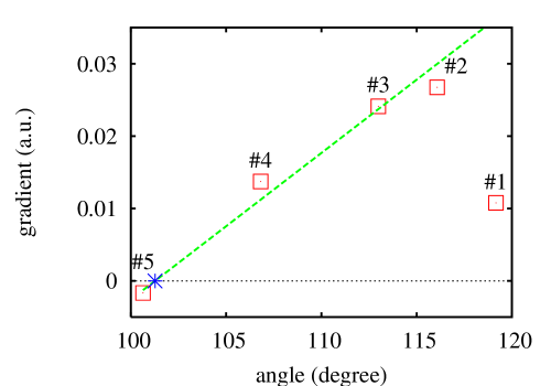
Figure 1: Progression of gradients on a valence angle bending coordinate of ammonia. Energies and forces have been obtained by the PBE density functional model in STO-3G basis set. The optimization was started from near planar geometry, i.e. from the vicinity of a transition state, and converged to a local minimum of the potential energy surface. The numbers in the picture indicate the sequence of optimization steps. The dashed line represents a linear fit, the star the predicted location of the minimum.

An observation central to the present contribution is that internal coordinate gradients show trends during optimization that can be captured by curve fitting and used to predict minima by one-dimensional extrapolation. This is illustrated in Fig. 1, showing a typical progression of internal coordinate gradients.

In the following, we review conventional methods of geometry optimization (Section II), and then develop our new idea conceptually (Section III). A practical implementation of this concept is then outlined (Section IV) in the context of linear scaling quantum chemistry. Next, this implementation is tested against Baker’s small molecule test suite and applied to a reaction model of Protein Kinase A (Section V).

I.1 Conventional Methods

Over the last three decades, internal coordinate geometry optimizers have become the standard tools for finding local minima when energies and forces are calculated by electronic structure theory. Internal coordinates describe the internal motions of molecules with chemical degrees of freedom such as bond-stretches, valence angle bendings and the torsions of dihedral angles. These curvilinear coordinates are constructed from non-linear functions of the Cartesian coordinates of atomic nuclei Wilson et al. (1955).

The reduced vibrational coupling achieved with internal coordinates provides an advantage in molecular geometry optimization Pulay (1977) and molecular dynamics Pulay and Paizs (2002). Specifically, a full Newton step in Cartesian coordinates will typically generate a larger, anharmonic coupling relative to a full Newton step carried out in internal coordinates. An excellent discussion of this issue can be found in the Introduction of Ref. Fogarasi et al., 1992.

Today, the most aggressive internal coordinate algorithms have been highly optimized for small molecule quantum chemistry. These methods typically generate a Cartesian Hessian, either exactly or approximately. This Cartesian Hessian is then transformed into an internal coordinate representation, and an internal coordinate Newton step is taken. The internal coordinate step is then transformed back to a Cartesian displacement and used to increment the molecular geometry.

There are many variations on this approach. Cartesian Hessians are usually calculated by updating algorithms in the framework of the variable metric or quasi-Newton approach such as the Broyden-Fletcher-Goldfarb-Shanno (BFGS) method Fletcher (1981). With increasing system size, storing, transforming and potentially inverting a full Hessian matrix scales as ${\cal O}(N^{3})$, and it becomes favorable to consider diagonal or semi-diagonal approximations to the internal coordinate Hessian. This severely truncated Newton or “force relaxation” method typically obtains static diagonal values a priori from spectroscopic data or empirical force-fields Pulay (1969); Pulay et al. (1979); Fogarasi et al. (1992); Pulay (1977); Sellers et al. (1978); Alsenoy et al. (1998); Lindh et al. (1995).

It is worth noting that the landmark RHF/4-21G optimization of Crambin by Van Alsenoy Alsenoy et al. (1998) was carried out in just 79 steps using the force relaxation approach of Sellers Sellers et al. (1978). In these algorithms, strong damping Sellers et al. (1978) or line searching Schlegel (1982) is required to avoid divergence. Another important technique to accelerate convergence of geometry optimization is the geometric DIIS (GDIIS) Császár and Pulay (1984). While geometric DIIS is a simple technique, its successful application may require many intricate modifications Farkas and Schlegel (2002). A recent review and comparison of these algorithms and their technical details can be found in Ref. Bakken and Helgaker, 2002.

II A New Concept

In the Newton-Raphson (NR) approach to geometry optimization, a correction $\delta{\bf x}$ to the Cartesian vector $\bf x$ of nuclear positions is found by solving a local second order expansion of the energy function, yielding $\delta{\bf x}=-{\bf g}\cdot{\bf h}^{-1}$, where $\bf h$ is the Hessian, a matrix of energy second derivatives with respect to nuclear displacement, and $\bf g$ is the gradient vector of energy first derivatives. Thus, a step along a specific element of $\bf x$ is coupled to all components of $\bf g$ through off-diagonal elements of $\bf h$. Alternatively, it is possible to work in the principal axis system of $\bf h$, or normal modes, which derive from eigenvectors of the Hessian. On an ideal harmonic surface the NR method remains exactly decoupled to all orders in the basis of normal modes, and also achieves quadratic convergence.

Now consider an approximate NR algorithm in a basis of diagonalizing normal modes, applied to a non-ideal anharmonic surface. For the moment, assume that the normal modes remain diagonalizing with each geometry step, but the eigenvalues change. Then, if the geometry steps are small, eigenvalues can be re-computed with backward differences of the gradient information at each step. With infinitesimal steps, this independent coordinate approximation is formally equivalent to NR.

Realistically though, both eigenvectors and eigenvalues of the Hessian will change as the algorithm takes the largest possible steps, leading to second (and higher) order coupling effects. At this point, we turn to an internal coordinate system to continue development of the independent coordinate approximation. In an internal coordinate system, the magnitude of harmonic and anharmonic coupling effects are small over the course of optimization. On the other hand, in a static basis of normal modes anharmonic coupling effects are larger to begin with Pulay et al. (1979), and coupling will increase during the course of optimization unless the normal modes are periodically recomputed, incurring an unacceptable cost for large systems.

Extending the independent coordinate approximation, it is clear that a differencing scheme will be inaccurate due to large step sizes. Also, because coordinate independence is an approximation, coupling effects will lead to scatter in the gradient data. Replacing the differencing scheme with a curve fit has the potential to both smooth the data and provide higher order accuracy. Using the local tangent of a fitted curve to approximate diagonal elements of the Hessian would be similar to force relaxation Pulay (1977); Sellers et al. (1978); Alsenoy et al. (1998), but with constantly updated values of the Hessian. However, the curve fit can be carried further; forsaking an approximate Newton step, the curve fit can be used instead to extrapolate or interpolate a zero for the parameterized gradient data. To first order (a line fit), this is equivalent to a one-dimensional Newton step with a fitted gradient and a fitted Hessian. While the approach outlined so far works well, the use of standard least squares is not optimal due to the ability of outliers to skew the fit. A significant advance can be realized by instead using a weighted curve fit, with the weights depending indirectly on estimation of local coupling effects.

We call this concept the “QUasi Independent Curvilinear Coordinate Approximation” or QUICCA.

Explicitly then, application of QUICCA to geometry optimization involves the projection of Cartesian gradient information onto an uncoupled $N_{\rm int}$ dimensional internal coordinate space. Energy gradients are accumulated for each internal coordinate, as shown in Fig. 1, and used to formulate $N_{\rm int}$ independent curves by weighted least squares. At each step, these curves are extrapolated (or interpolated) to zero, with collective changes in the internal coordinate system taken as an approximate minima for the system as a whole. The final back-transformation of the step to Cartesian coordinates merges these displacements, reconciling any redundancies in the internal coordinate system. The quality of this collective extrapolation is determined by severity of the low order coupling, redundancy of the internal coordinate system and the accuracy of the fit. The QUICCA approach to geometry optimization is simple to implement and scales linearly with system size. It overcomes low order coupling effects through averaging and weighting of the curve fit and also admits the accumulation of anharmonic information. However, augmenting QUICCA with anharmonic quadratic and higher order terms and preserving the important smoothing effect of the weighted fit is an advanced subject beyond the scope of this work.

III Implementation

III.1 Recognition of Internal Coordinates

The present implementation of QUICCA employs a redundant set of primitive internal coordinates. Similar coordinate systems are used by a majority of other internal coordinate optimizers Fogarasi et al. (1992); Pulay et al. (1979); Baker (1993); Eckert et al. (1997); Farkas and Schlegel (1998). The generation of these coordinates starts with the recognition of covalent bonds, based on atomic Slater radii Slater (1964) multiplied by an empirical factor of 1.3. Weak bonds are recognized on the basis of atomic van der Waals (VDW) radii JMO (2004). Note, that no VDW contact is allowed between atoms, which are second or third neighbors in the covalent bonding scheme. The search for neighboring atoms is carried out by dividing the system into small cubes a few angstroms on a side, and bonds are looked for only within each box and between nearest neighbor boxes. This divide-and-conquer scheme ensures the fast and linear scaling recognition of bonding for large molecules. The bonding scheme is then stored as the symbolic component (graph) of the sparse topology matrix.

At each step of the optimization, the bonding scheme is determined and the corresponding primitive topology matrix is stored. Then, primitive topology matrices from the $n_{\rm fit}$ most recent steps are summed to yield a merged topology matrix, where $n_{\rm fit}$ is the same number of points employed by the curve fitting. In the current implementation $n_{\rm fit}=7$, but it can be much larger or smaller.

The merged topology matrix avoids fluctuations due to the possibility of bond-formation and bond vanishing during the optimization of large molecules. Use of the merged topology matrix increases the number of internal coordinates and the redundancy of the coordinate set only slightly; the final merged topology matrix is determined directly from primary topology matrices rather than the merged ones at previous cycles.

Based on the topology matrix of the merged bonding network, all other primitive internal coordinates, such as bond angles, torsions, linear bendings and out-of-planes are recognized. Torsions are selected so that each bond will be associated with only a single torsional coordinate.

III.2 Preparing the Data

Cartesian coordinates and the corresponding Cartesian gradients of the $n_{\rm fit}=7$ most recent geometries are read from disk. Based on the most recent definition of the bonding scheme they are transformed into the internal coordinate representation, determined by the merged bonding scheme. The coordinate transformation is carried out as described in Ref. Németh et al., 2000, while the necessary intermediate sparse matrices of the coordinate transformation are re-generated. This is a very inexpensive step, due to the extreme sparsity of the vibrational B matrix Wilson et al. (1955). Thus the primary objects of the proposed geometry optimization, the internal coordinates and their gradients, are re-created at each step allowing on-the-fly redefinition of the coordinate system.

In order to avoid problems due to the periodicity of torsional angles, reference points are used, eg. the torsional angle values of the most recent geometry. Each torsional angle is set to its periodic equivalent closest to the reference point, by a shift of $\pm 2\pi$, while its gradient value does not change.

III.3 The Weighted Curve Fit

At this point, we have a set of $n_{\rm fit}$ coordinate - gradient pairs for each individual internal coordinate, such as the one presented in Fig. 1. These data pairs parametrize progression of the gradient during the $n_{\rm fit}$ most recent steps of the optimization. This data is now used to fit curves for each of the $N_{\rm int}$ coordinates using the SLATEC routine POLFIT and its dependencies sla (1993), which perform a weighted least squares fit.

The choice of weight is a key factor in the behavior of the QUICCA algorithm, as it is used to prioritize reliable portions of the data and to generally smooth noisy trends. Originally, we considered the standard expression $w_{k}^{(i)}=\left(1/{g_{k}^{(i)}}\right)^{2}$ for the weight of the $k$-th internal coordinate at the $i$-th geometry, which is generally recommended for use in curve fitting Press et al. (1992). These weights however do not account for the fact that the gradient of the $k$-th internal coordinate may be small, while its immediate environment may contain large gradients indicating the possibility of large changes in the $k$-th internal coordinate due to coupling effects. Thus, a data point with high environmental tension is less reliable than a point with neighboring coordinates that are relaxed. Local sums of the gradient squares,

$$w_{k}^{(i)}=\left[\sum_{l}g_{l}^{(i)}\frac{1}{|H_{ll}|}g_{l}^{(i)}\right]^{-1},$$ (1)

incorporate this effect, where $l$ indexes internal coordinates that have atoms in common with the $k$-th internal coordinate, and $H_{ll}$ is an approximate, static approximation to the diagonal Hessian. The terms $H_{ll}$ yield dimensionally consistent sums, since each of the gradient components $g_{l}$ has a different measure and energy scale for stretches, bendings and torsions.

For each coordinate $k$, the sum over $l$ is determined by the topology matrix, given by the symbolic structure (graph) of the sparse matrix $G_{i}=BB^{t}$, which obtains from the sparse Wilson’s $B$ matrix Wilson et al. (1955). We have considered more delocalized interactions as well, such as those deriving from the graph of $G_{i}^{2}$, but they did not provide any significant improvement in test calculations.

Values of $1.0$ au for stretches, $0.1$ au for bendings (and linear bendings and out-of-planes) and $0.01$ au for torsions are used for the $H_{ll}$. These values are similar to those used to provide an initial guess for the Hessian in variable metric algorithms Bakken and Helgaker (2002). Note, that only the relative values of $H_{ll}$ are important for the fitting process, as the fitting parameters are determined by the relative values of the weights.

While it is possible to employ second and third order polynomials in the fit, in our current implementation extrapolation to zero is most robust with just a line. A primary difficulty in the construction of higher order fits is that distinguishing between noise and signal is more difficult. Also, there are stability issues of extrapolation versus interpolation with higher order polynomials. Thus while we believe there is opportunity for higher order approximations, their development is beyond the scope of the present paper.

III.4 Minimum or Transition State?

Transition states are indicated by a gradient curve with negative tangent at the position of the root. For example, in Fig. 1 the tangent of the gradient curve is negative in the vicinity of the planar structure (structure #1), which is a transition state. The tangent of the gradient curve thus offers a convenient tool to control convergence to either a minimum or transition state. Whenever the local tangent of the gradient curve is negative, the optimizer employs a simple force relaxation step,

$$\varphi_{k}^{(i+1)}=\varphi_{k}^{(i)}-g_{k}^{(i)}/|H_{kk}^{(i)}|,$$ (2)

where $i$ denotes the serial number of the optimization step, $\varphi_{k}$ is the $k$-th internal coordinate, $H^{(i)}_{kk}$ is a diagonal element of the Hessian determined from local tangent of the curve fit, and $g_{i}$ is the local gradient at $i$ (not a fitted gradient). This avoids transition states that are well localized to just a few internal coordinates. The ability of the present implementation to treat delocalized transition states remains to be seen.

Combined internal coordinates, such as the natural Fogarasi et al. (1992) or the delocalized internals Baker et al. (1996), hold the possibility of identifying delocalized transition states by gradient fitting. An analysis by Wales et.al. Uppenbrink and Wales (1992) provides insight into the numerical problems involved in controlling convergence to a minimum without an accurate Hessian. Note that, even with a good quality Hessian update, such as BFGS Fletcher (1981), there is no guarantee to converge into a minimum instead of a transition state. This is because positive definiteness of an approximate Hessian does not guarantee the positive definiteness of the exact Hessian. Thus, the exact Hessian remains the only absolute for determining the character of extremal points in the potential energy surface Fogarasi et al. (1992).

III.5 Initial steps

In the very first step of the optimization, a force relaxation step is used with the usual diagonal Hessian estimates of 0.5 au for stretchings, 0.2 au for bendings and 0.1 au for torsions. This initial step is equivalent with the one traditional optimizers use.

III.6 Step size control and backtracking

Experience with QUICCA has shown that extrapolations larger than the range spanned by the fitted data points are unreliable. Thus, while QUICCA always tries to achieve the predicted minimum, stepsize control is imposed, limiting the step by the fit range or to 0.3 au, whichever is less. This maximum allowed value of the stepsize, 0.3 au, is similar to that used by other optimizers Eckert et al. (1997).

The range spanned by the fitted data is in some sense an uncertainty. Refining and formalizing quantification of this uncertainty is another area of opportunity for improvement of the QUICCA optimizer, which is beyond the scope of this article. We note however, that it might be more effective to use a filtered range of the data points, based on their weights. For example, compute the range including only those points with weights that comprise, say, 99.99 percent of the total. Alternatively, statistical tests could be employed to filter out outlying points. We note that issues of uncertainty in stepsize control are certain to be far more complex for higher order fits, and advanced statistical methods may have a significant role to play in this area of development.

III.7 Backtracking

While the above stepsize control is designed to avoid potential instabilities, it is still possible to take steps that will increase the total energy. In this case, there are a number of options. We can live with the increase, hoping it will nevertheless improve the information content used to build the energy surface. We can backtrack, uniformly reducing the step, typically by half, and re-evaluate the energy to see if it decreases. Alternatively, we can employ a more sophisticated and expensive line search to determine a minimizing step.

There are many ways to carry out a line-search. Perhaps the most widely employed approach is the endpoint algorithm of Schlegel Schlegel (1982). This algorithm employs energies and gradients at the endpoints to yield a quartic interpolant. This approach will work well if the interpolant varies smoothly between endpoints. We have implemented this approach to the line-search, but found that it does not perform reliably, especially when large steps are made. It may be that midpoint algorithms are more appropriate, but we have not explored this further.

Our experience with QUICCA is that simple back-tracking is both cheaper and more effective than the endpoint line-search. During back-tracking, a bad step is recognized by an elevated energy before any gradient evaluation takes place. Then, the step-size is halved, and a new energy is calculated. This process is repeated until the energy becomes lower, typically requiring just one halving.

III.8 Iterative back-transformation

Once predictions of internal coordinate displacements are made, they are passed to the iterative back-transformation to generate a new set of Cartesian coordinates, as in Ref. Pulay, 1977. However, there is no guarantee that there exists a set of Cartesian coordinates that can exactly realize the new, predicted internal coordinates. For example, a prediction of angles in a triangular molecule can sum to a value greater than or less than 180 degrees. Such conflicts are a consequence of the redundant internal coordinate system.

Displacements in the updated internal coordinate system that result in geometric conflicts will be projected out during the iterative back-transformation. However, if these conflicts are too large, the iterative back-transformation may fail to converge, or it may produce a set of Cartesian coordinates that violates the predicted internal coordinate values. Typically, these violations are big when stepsizes are large, but become small close to convergence.

One approach to avoiding this problem is to work with linear-combinations of primitive internal coordinates, such as the natural Fogarasi et al. (1992) or delocalized Baker et al. (1996) internal coordinates, which minimize geometric conflicts. Another cure for redundancies is to apply a projection technique prior to the iterative-back transformation Pulay (1977), which can eliminate problems to first-order, but does not guarantee convergence for large steps.

In our present implementation, geometric conflicts are dealt with solely by the iterative back-transformation. In the case of non-convergent back-transformation, our algorithm will attempt the back-transformation again, but with the original internal coordinate displacements halved. If the repeated transformation also fails, it usually indicates an incomplete set of internal coordinates and the program stops. An incomplete set can also scuttle convergence of the Cartesian to internal gradient transformation Németh et al. (2000). Note, that an appropriate internal coordinate recognition program together with suitable internal coordinate step-size control can always avoid the non-convergent back-transformation.

III.9 Realization

The QUICCA geometry optimization algorithm has been implemented in the object oriented FORTRAN-90/95 programming language and is part of the MondoSCF suite of linear scaling quantum chemistry codes Challacombe et al. (2001). It has been successfully tested on different platforms, compilers and operating systems.

III.10 Scaling

At each geometry step, the cost of QUICCA is associated only with recognition of internal coordinates, the coordinate transformations and the fitting process. The recognition of internal coordinates scales linearly, as described in Section IV A. The effort spent on fitting is ${\cal O}(N_{\rm int})$ with $N_{\rm int}\propto N_{\rm atoms}$, as the number of points employed by each fit is a constant. Likewise, the coordinate transformations scale linearly with system size as pointed out in Ref. Németh et al., 2000.

IV Results and Discussion

Table 1: Number of geometry optimization steps to convergence of Baker’s test set (up to 30 atom molecules) for the QUICCA optimizer and also for other advanced algorithms from the literature. Calculations have been carried out at the RHF/STO-3G level of theory. All of the reported calculations used local primitive internal coordinates, except those of Bakken et.al. who used extra redundant coordinates Bakken and Helgaker (2002).

Molecule	QUICCA	Bakken	Eckert	Lindh	Baker
		et al.	et al.	et al.
		Bakken and Helgaker (2002)	Eckert et al. (1997)	Lindh et al. (1995)	Baker (1993)
Water	4	4	4	4	6
Ammonia	4	5	6	5	6
Ethane	4	3	4	4	5
Acetylene	4	4	6	5	6
Allene	3	4	4	5	5
Hydroxysulphane	8	7	7	8	8
Benzene	2	3	3	3	4
Methylamine	4	4	5	5	6
Ethanol	5	4	5	5	6
Acetone	4	4	5	5	6
Disilyl ether	9	8	9	11	8
1,3,5-trisilacycl.	5	9	6	8	8
Benzaldehyde	5	4	5	5	6
1,3-difluorobenz.	4	4	5	5	5
1,3,5-trifluorob.	3	4	4	4	5
Neopentane	5	4	4	5	5
Furan	6	5	6	7	8
Naphtalene	6	5	6	6	5
1,5-difluoronapht.	6	5	6	6	6
2-hydroxibicyclop.	7	9	9	10	15
ACHTAR10	10	8	9	8	12
ACANIL01	11	7	8	8	8
Benzidine	8	9	7	10	9
Pterin	12	8	9	9	10
Difuropirazine	6	6	7	7	9
Mesityl oxide	5	5	6	6	7
Histidine	11	16	14	20	19
Dimethylpenthane	6	9	10	10	12
Caffeine	7	6	7	7	12
Menthone	13	12	10	14	13
Total	187	185	196	215	240

IV.1 Baker’s test set

The performance of the QUICCA optimizer has been tested on Baker’s suite Baker (1993) of small test molecules, and is listed in Table 1, along with values from more traditional algorithms. At convergence, the magnitude of the maximum Cartesian force vector is required to be less than $3\times 10^{-4}$ au for each atom. This criterion is tighter than that employed in other studies Ref. Baker, 1993, which require only that the maximum Cartesian force component (X, Y or Z) be less than $3\times 10^{-4}$ au. In addition to this criterion, an absolute energy change less than $1\times 10^{-6}$ au or a predicted internal coordinate displacement less than $3\times 10^{-4}$ au at the last geometry is required. The energies of the optimized structures have been reproduced to all digits given in Ref. Baker, 1993.

The current implementation of QUICCA, achieving a total of 187 geometry steps for Baker’s test suite, is competitive with Bakken’s algorithm, requiring 185.

Bakken’s method Bakken and Helgaker (2002) derives from an optimal combination of advanced techniques related to internal coordinate methods based on a dense Cartesian Hessian update. It involves a Cartesian BFGS update Fletcher (1981), the Rational Function Optimization scheme Banerji et al. (1985) and a Newton trust-region model Fletcher (1981). An important addition to these techniques is the extra redundant coordinates, which contribute to the success of Bakken’s algorithm relative to more traditional schemes. Extra redundant internal coordinates are local distance coordinates, which bridge the terminal atoms of all valence angles and most of the dihedral angles.

In contrast, the current implementation of QUICCA employs a redundant primitive internal coordinate system, a weighted line fit and simple backtracking.

In two cases (ACANIL01 and Pterin), the QUICCA optimizer proved to be considerably slower than the best traditional techniques. We believe these cases may be improved by introducing a more sensitive weighting scheme, and/or employing a more sophisticated internal coordinate system as discussed above in Section IV H.

Note that these results have been achieved without the use of traditional convergence acceleration algorithms such as geometric DIIS (GDIIS) Császár and Pulay (1984); Farkas and Schlegel (2002). It is of course entirely possible to deploy the GDIIS algorithm together with QUICCA, but we leave this avenue open for future work.

Our experience shows, that QUICCA is relatively insensitive to the values of $H_{ll}$ employed in the construction of weights (see Section IV C). For example the values $0.5$, $0.2$ and $0.1$ au for $H_{ll}$ (instead of our standard, $1.0$, $0.1$ and $0.01$ au) resulted in 189 steps instead of 187 for Baker’s test set. The largest difference was present in Dimethylpenthane, which converges 2 steps faster when using the standard $H_{ll}$ values.

In Baker’s test suite, about three force evaluations have been saved by using backtracking. Without the application of backtracking, Baker’s test set converges in 190 steps. This suggests that the core QUICCA algorithm is robust and does not often overstep.

We can understand the stability achieved by the core QUICCA algorithm by considering a hybrid force relaxation method, based on Eq. 2, in which the diagonal Hessian elements $H^{(i)}_{kk}$ are obtained from the curve fit, but the uncoupled Newton step is carried out with the current gradient. We have tested this alternative, but it turned out to be oscillatory in many cases, requiring excessive backtracking. This should be contrasted with the full QUICCA algorithm, which uses extrapolation. To first order this is equivalent with an approximate Newton step taken with the fitted gradient. Thus, the full QUICCA algorithm is successful not only because it generates up-to-date curvature information, but because it achieves stability through smoothing effects derived from the weighted fit.

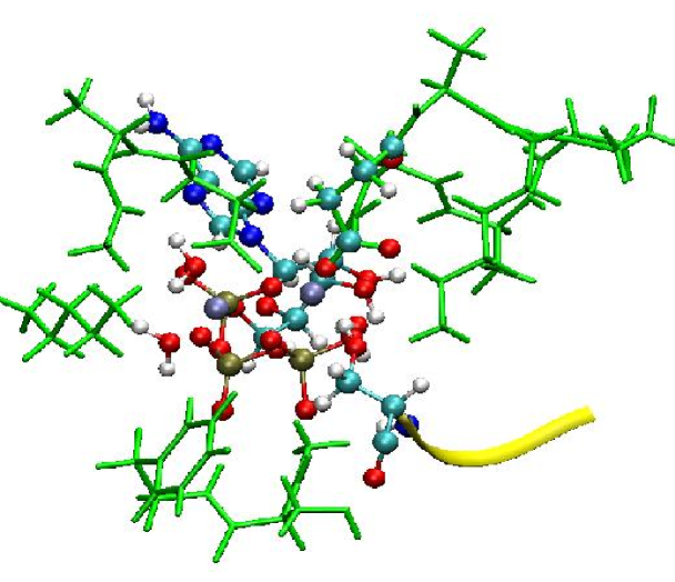
Figure 2: The structure of a 263 atom Protein Kinase A fragment used to test the QUICCA optimizer.

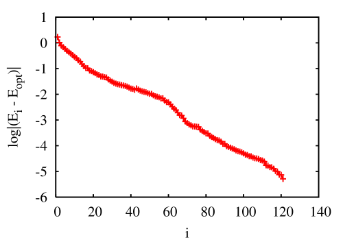
Figure 3: Convergence of the energy with geometry step $i$ on a log₁₀-linear scale for the 263 atom Protein Kinase A fragment at the RHF/STO-2G level of theory.

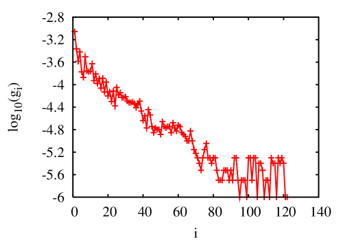
Figure 4: Convergence of the root mean square of the Cartesian gradients, $g_{i}$, with geometry step $i$ on a log₁₀-linear scale for the 263 atom Protein Kinase A fragment at the RHF/STO-2G level of theory.

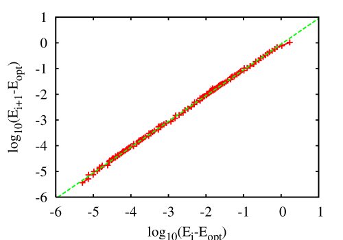
Figure 5: A plot of ${\rm log}_{10}\Delta E_{i+1}$ vs ${\rm log}_{10}\Delta E_{i}$, characterizing the ratio $\Delta E_{i+1}/\Delta E_{i}$. The solid line is $y=-0.04980+1.00111*x$. The slope of this line is equivalent to the order of convergence ($n=1.00111$), while the y-intercept is the negative rate of convergence ($-f={\rm log}_{10}(c)=-0.04980$).

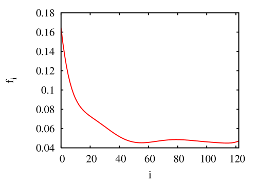
Figure 6: Change in the rate of convergence $f$ during optimization of the 263 atoms Protein Kinase A fragment. $f$ is modeled by a 10th order polynomial. The polynomial coefficients have been obtained from a non-linear fit to the $E_{i}$-$i$ data-pairs, using the model function $E_{i}=E_{\rm opt}+A*e^{-f*i}$.

IV.2 Convergence

Away from the basin of attraction, both steepest descents as well as the Newton-Raphson algorithm converge linearly. However, these methods behave very differently when condition number of the Hessian is large, for example when low frequency “floppy” modes are present. In this case, steepest descents can be extremely slow, while second order (Newton-Raphson) and approximate second order (quasi-Newton) methods achieve an accelerated rate of convergence through conditioning of the stepsize. While methods that render the number of geometry steps independent of system size do exist Goedecker et al. (2001), they apply (so far) only to homogeneous systems. In general though, the number of steps required to minimize to within a certain tolerance increases with system size, roughly as ${\cal O}(N_{\rm atoms}/3)$ according to Ref. Daniels et al., 2000. Therefore, the rate of linear convergence achieved by an optimization algorithm is perhaps a good measure of performance for large systems.

An optimization algorithm may be characterized by the ratio ${\Delta E_{i+1}}/{\Delta E_{i}^{n}}=c$, where $\Delta E_{i}=|E_{i}-E_{\rm opt}|$ is the absolute error at geometry step $i$, $E_{\rm opt}$ is the extremal value of the energy, $n$ is the order of convergence, and $c$ is the convergence factor Quarteroni et al. (2000). With first order convergence $n=1$, and the error typically decays exponentially as $\Delta E_{i}=e^{-f_{i}*i}$, where $f=-{\rm log}(c)$ is the rate of convergence. In the basin of attraction, where the second order approximation to the nonlinear objective is accurate, the Newton-Raphson method achieves second order convergence, $n=2$, while approximate second order methods (quasi-Newton algorithms for example) can at best achieve superlinear convergence Fletcher (1981); Fogarasi et al. (1992). Superlinear convergence is characterized by $n=1$ and an increasing rate of convergence $f$, equivalent to $\lim_{i\to\infty}c_{i}=0$.

To investigate the convergence properties of QUICCA in a large application, we have carried out optimization of a 263 atom fragment of crystallographic Protein Kinase A, involving two Magnesiums, three crystallographic waters, ATP and a fragment of the Protein Kinase Inhibitor to which phosphate is transfered. This is a model reactant system obtained from Ref. Helkelman et al., 2004 and is shown in Fig. 2. Optimization was performed at the HF/STO-2G level of theory with an approximate absolute energy resolution of $10^{-5}$ hartree using MondoSCF Challacombe et al. (2001) at the tight accuracy level and with ten peripheral atoms constrained to mimic steric effects of the enzyme. Note that this minimal level of theory actually makes more work for the optimizer, as it will tend to move away from the more correct crystallographic structure. This structure was optimized to within a Cartesian force of $3\times 10^{-4}$ au and a maximum predicted displacement less than $4\times 10^{-3}$ au. The number of internal coordinates, generated for this structure was 1280 at convergence. Figure 3 shows ${\rm log}_{10}\Delta E_{i}$ vs $i$ for this system, Fig. 4 the root mean square of the Cartesian gradient at each step.

In Fig. 5, a plot of ${\rm log}_{10}{\Delta E_{i+1}}$ vs ${\rm log}_{10}{\Delta E_{i}}$ is shown, demonstrating only first order convergence with a rate $f\sim 0.05$. To examine the rate of convergence in greater detail, we fit the the model function $E_{i}=E_{\rm opt}+A*e^{-i*f_{i}}$, using an 11th order polynomial to represent $f_{i}$. The fitted rate of convergence shown in Fig. 6 suggests that the optimization has three different phases, in accordance with Fig. 3. In the first phase (steps 1-10) there is a rapid refinement of the least-optimal substructures. In the second phase (steps 10-60) the absolute energy decreases less rapidly to $\sim 1$ mhartree, with the main optimization effort corresponding to changes in the local internal coordinates. Finally, the third phase (60-120) occurs at a slower, constant rate of about $f=0.05$, which is consistent with the fit characterizing the ratio ${\Delta E_{i+1}}/{\Delta E_{i}}$ shown in Fig. 5.

In the third phase, below 1 mhartree, backtracking becomes necessary to achieve smooth convergence of the energy and the rate of convergence decreases to a constant. We believe that this deceleration is due to the presence of “floppy” low-frequency modes that are highly delocalized and not accounted for in the current local internal coordinate system. While QUICCA can certainly be used with a more delocalized internal coordinate system, the construction of delocalized internal coordinates is an important open problem in molecular geometry optimization. It is also important to note that the effect of floppy modes is not the only factor in the third phase of the optimization; the rigidity of the internal coordinate system and its role in the inaccurate convergence of the back-transformation is also important. In our opinion, these two factors, which characterize the last phase of the optimization may be related to each other. A recent work of Fernandez-Serra et.al Fernandez-Serra et al. (2003) calls attention to the relationship of the rigidity of internal coordinate systems and the phenomenon of floppy modes. This relationship may be understood from the theory of rigidity Phillips and Thorpe (1985). In the present work, we do not consider this relationship further.

V Conclusions

We have presented a new concept for local optimization, the “QUasi Independent Curvilinear Coordinate Approximation” or QUICCA, and applied it to the geometry optimization of molecular structures. Competitive with the most aggressive internal coordinate geometry optimizers in the literature, QUICCA has demonstrated that an efficient optimization algorithm can be constructed without explicit coupling in local expansion of the energy. However, coupling effects do enter QUICCA implicitly through the weighted curve fit, providing an important averaging effect that compensates for irregularities related to the independent coordinate approximation.

The implementation presented here is relatively simple, employing redundant primitive internal coordinates, a weighted line fit and backtracking, allowing substantial room for improvement. Indeed, the QUICCA concept opens the door for a wide range of auxiliary techniques that may benefit from physical insight (such as the development of more precise weighting schemes) as well as from ideas in applied mathematics involving robust estimation, interpolation and advanced methods of regression.

The primitive internal coordinate system employed in the present implementation does not include delocalized motions and suffers from slowdowns associated with floppy modes. The construction of delocalized internal coordinate systems that remain approximately decoupled is thus an outstanding problem in molecular geometry optimization. Nevertheless, the preconditioning afforded by local stretchings, bendings and torsions is an important step, enabling the large scale application of linear scaling electronic structure theory to problems in biology and materials science. In addition, with the availability of fast linear scaling Cartesian/internal coordinate transforms Németh et al. (2000), the QUICCA algorithm may also present advantages in the optimization of large systems employing classical forcefields.

The averaging scheme presented here, achieving an effective decoupled internal coordinate representation of the potential energy surface, may also be useful in on-the-fly construction of classical force fields. In such an approach, force field parameters such as the spring-constant and equilibrium position could be updated periodically from ab initio data, taken over several time steps. This on-the-fly construction of force fields based on QUICCA might provide a useful alternative to the force matching algorithm of Ercolessi et.al. Ercolessi and Adams (1994) and to the reactive force field concepts developed by the Goddard group van Duin et al. (2001a, b).