String-net condensation: A physical mechanism for topological phases

Abstract

We show that quantum systems of extended objects naturally give rise to a large class of exotic phases - namely topological phases. These phases occur when the extended objects, called “string-nets”, become highly fluctuating and condense. We derive exactly soluble Hamiltonians for 2D local bosonic models whose ground states are string-net condensed states. Those ground states correspond to 2D parity invariant topological phases. These models reveal the mathematical framework underlying topological phases: tensor category theory. One of the Hamiltonians - a spin-1/2 system on the honeycomb lattice - is a simple theoretical realization of a fault tolerant quantum computer. The higher dimensional case also yields an interesting result: we find that 3D string-net condensation naturally gives rise to both emergent gauge bosons and emergent fermions. Thus, string-net condensation provides a mechanism for unifying gauge bosons and fermions in 3 and higher dimensions.

I Introduction

For many years, it was thought that Landau’s theory of symmetry breaking Landau (1937) could describe essentially all phases and phase transitions. It appeared that all continuous phase transitions were associated with a broken symmetry. However, after the discovery of the fractional quantum Hall (FQH) effect, it was realized that FQH states contain a new type of order - topological order - that is beyond the scope of Landau theory (for a review, see LABEL:Wtoprev). Since then the study of topological phases in condensed matter systems has been an active area of research. Topological phases have been investigated in a variety of theoretical and experimental systems, ranging from FQH systems Wen and Niu (1990); Blok and Wen (1990); Read (1990); Fröhlich and Kerler (1991), quantum dimer models Rokhsar and Kivelson (1988); Read and Chakraborty (1989); Moessner and Sondhi (2001); Ardonne et al. (2004) , quantum spin models Kalmeyer and Laughlin (1987); Wen et al. (1989); Wen (1990); Read and Sachdev (1991); Wen (1991a); Senthil and Fisher (2000); Wen (2002); Sachdev and Park (2002); Balents et al. (2002), to quantum computing Kitaev (2003); Ioffe et al. (2002), or even superconducting states Wen (1991b); Hansson et al. (2004). This work has revealed a host of interesting theoretical phenomena and applications, including fractionalization, anyonic quasiparticles, and fault tolerant quantum computation. Yet, a general theory of topological phases is lacking.

One way to reveal the gaps in our understanding is to compare with Landau’s theory of symmetry breaking phases. Landau theory is based on (a) the physical concepts of long range order, symmetry breaking, and order parameters, and (b) the mathematical framework of group theory. These tools allow us to solve three important problems in the study of ordered phases. First, they provide low energy effective theories for general ordered phases: Ginzburg-Landau field theories Ginzburg and Landau (1950). Second, they lead to a classification of symmetry-breaking states. For example, we know that there are only 230 different crystal phases in three dimensions. Finally, they allow us to determine the universal properties of the quasiparticle excitations (e.g. whether they are gapped or gapless). In addition, Landau theory provides a physical picture for the emergence of ordered phases - namely particle condensation.

Several components of Landau theory have been successfully reproduced in the theory of topological phases. For example, the low energy behavior of topological phases is relatively well understood on a formal level: topological phases are gapped and are described by topological quantum field theories (TQFT’s).Witten (1989a) The problem of physically characterizing topological phases has also been addressed. LABEL:Wtoprev investigated the “topological order” (analogous to long range order) that occurs in topological phases. The author showed that topological order is characterized by robust ground state degeneracy, nontrivial particle statistics, and gapless edge excitations.Wen (1990); Wen and Niu (1990); Wen (1992) These properties can be used to partially classify topological phases. Finally, the quasiparticle excitations of topological phases have been analyzed in particular cases. Unlike the symmetry breaking case, the emergent particles in topologically ordered (or more generally, quantum ordered) states include (deconfined) gauge bosonsBanks et al. (1977); Foerster et al. (1980) as well as fermions (in three dimensions) Levin and Wen (2003); Wen (2003a) or anyons (in two dimensions) Arovas et al. (1984). Fermions and anyons can emerge as collective excitations of purely bosonic models.

Yet, the theory of topological phases is still incomplete. The theory lacks two important components: a physical picture (analogous to particle condensation) that clarifies how topological phases emerge from microscopic degrees of freedom, and a mathematical framework (analogous to group theory) for characterizing and classifying these phases.

In this paper, we address these two issues for a large class of topological phases which we call “doubled” topological phases. On a formal level, “doubled” topological phases are phases that are described by a sum of two TQFT’s with opposite chiralities. Physically, they are characterized by parity and time reversal invariance. Examples include all discrete lattice gauge theories, and all doubled Chern-Simons theories. It is unclear to what extent our results generalize to chiral topological phases - such as in the FQH effect.

We first address the problem of the physical picture for doubled topological phases. We argue that in these phases, local energetic constraints cause the microscopic degrees of freedom to organize into effective extended objects called “string-nets”. At low energies, the microscopic Hamiltonian effectively describes the dynamics of these extended objects. If the kinetic energy of the string-nets dominates the string-net tension, the string-nets “condense”: large string-nets with a typical size on the same order as the system size fill all of space (see Fig. 1). The result is a doubled topological phase. Thus, just as traditional ordered phases arise via particle condensation, topological phases originate from “string-net condensation.”

Figure 1: A schematic phase diagram for the generic string-net Hamiltonian (3). When $t/U$ (the ratio of the kinetic energy to the string tension) is small the system is in the normal phase. The ground state is essentially the vacuum with a few small string-nets. When $t/U$ is large the string-nets condense and large fluctuating string-nets fill all of space. We expect a phase transition between the two states at some $t/U$ of order unity. We have omitted string labels and orientations for the sake of clarity.

This physical picture naturally leads to a solution to the second problem - that of finding a mathematical framework for classifying and characterizing doubled topological phases. We show that each topological phase is associated with a mathematical object known as a “tensor category.” Kassel (1995) Here, we think of a tensor category as a $6$ index object $F^{ijk}_{lmn}$ which satisfies certain algebraic equations (8). The mathematical object $F^{ijk}_{lmn}$ characterizes different topological phases and determines the universal properties of the quasiparticle excitations (e.g. statistics) just as the symmetry group does in Landau theory. We feel that the mathematical framework of tensor categories, together with the physical picture of string-net condensation provides a general theory of (doubled) topological phases.

Our approach has the additional advantage of providing exactly soluble Hamiltonians and ground state wave functions for each of these phases. Those exactly soluble Hamiltonians describe local bosonic models (or spin models). They realize all discrete gauge theories (in any dimension) and all doubled Chern-Simons theories (in $(2+1)$ dimensions). One of the Hamiltonians - a spin-1/2 model on the honeycomb lattice - is a simple theoretical realization of a fault tolerant quantum computer Freedman et al. (2002). The higher dimensional models also yield an interesting result: we find that $(3+1)D$ string-net condensation naturally gives rise to both emerging gauge bosons and emerging fermions. Thus, string-net condensation provides a mechanism for unifying gauge bosons and fermions in $(3+1)$ and higher dimensions.

We feel that this constructive approach is one of the most important features of this paper. Indeed, in the mathematical community it is well known that topological field theory, tensor category theory and knot theory are all intimately related Turaev (1994); Witten (1989b, 1990). Thus it is not surprising that topological phases are closely connected to tensor categories and string-nets. The contribution of this paper is our demonstration that these elegant mathematical relations have a concrete realization in condensed matter systems.

The paper is organized as follows. In sections II and III, we introduce the string-net picture, first in the case of deconfined gauge theories, and then in the general case. We argue that all doubled topological phases are described by string-net condensation.

The rest of the paper is devoted to developing a theory of string-net condensation. In section IV, we consider the case of $(2+1)$ dimensions. In parts A and B, we construct string-net wave functions and Hamiltonians for each $(2+1)D$ string-net condensed phase. Then, in part C, we use this mathematical framework to calculate the universal properties of the quasiparticle excitations in each phase. In section V, we discuss the generalization to $3$ and higher dimensions. In the last section, we present several examples of string-net condensed states - including a spin-1/2 model theoretically capable of fault tolerant quantum computation. The main mathematical calculations can be found in the appendix.

II String-nets and gauge theories

In this section, we introduce the string-net picture in the context of gauge theory Kogut and Susskind (1975); Banks et al. (1977); Wen (2003b). We point out that all deconfined gauge theories can be understood as string-net condensates where the strings are essentially electric flux lines. We hope that this result provides intuition for (and motivates) the string-net picture in the general case.

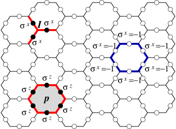
Figure 2: The constraint term $\prod_{\text{legs of }\boldsymbol{I}}\sigma^{x}_{\boldsymbol{i}}$ and magnetic term $\prod_{\text{edges of }\boldsymbol{p}}\sigma^{z}_{\boldsymbol{j}}$ in $Z_{2}$ lattice gauge theory. In the dual picture, we regard the links with $\sigma^{x}=-1$ as being occupied by a string, and the links with $\sigma^{x}=+1$ as being unoccupied. The constraint term then requires the strings to be closed - as shown on the right.

We begin with the simplest gauge theory - $Z_{2}$ lattice gauge theory Wegner (1971). The Hamiltonian is

$$H_{Z_{2}}=-U\sum_{\boldsymbol{i}}\sigma^{x}_{\boldsymbol{i}}+t\sum_{\boldsymbol{p}}\prod_{\text{edges of }\boldsymbol{p}}\sigma^{z}_{\boldsymbol{j}}$$ (1)

where $\sigma^{x,y,z}$ are the Pauli matrices, and $\boldsymbol{I}$, $\boldsymbol{i}$, $\boldsymbol{p}$ label the sites, links, and plaquettes of the lattice. The Hilbert space is formed by states satisfying

$$\prod_{\text{legs of }\boldsymbol{I}}\sigma^{x}_{\boldsymbol{i}}|\Phi\rangle=|\Phi\rangle,$$ (2)

for every site $\boldsymbol{I}$. For simplicity we will restrict our discussion to trivalent lattices such as the honeycomb lattice (see Fig. 2).

It is well known that $Z_{2}$ lattice gauge theory is dual to the Ising model in $(2+1)$ dimensions Kogut (1979). What is less well known is that there is a more general dual description of $Z_{2}$ gauge theory that exists in any number of dimensions Itzykson et al. (1988). To obtain this dual picture, we view links with $\sigma^{x}=-1$ as being occupied by a string and links with $\sigma^{x}=+1$ as being unoccupied. The constraint (2) then implies that only closed strings are allowed in the Hilbert space (Fig. 2).

In this way, $Z_{2}$ gauge theory can be reformulated as a closed string theory, and the Hamiltonian can be viewed as a closed string Hamiltonian. The electric and magnetic energy terms have a simple interpretation in this dual picture: the “electric energy” $-U\sum_{\boldsymbol{i}}\sigma^{x}_{\boldsymbol{i}}$ is a string tension while the “magnetic energy” $t\sum_{\boldsymbol{p}}\prod_{\text{edges of }\boldsymbol{p}}\sigma^{z}_{\boldsymbol{j}}$ is a string kinetic energy. The physical picture for the confining and deconfined phases is also clear. The confining phase corresponds to a large electric energy and hence a large string tension $U\gg t$. The ground state is therefore the vacuum configuration with a few small strings. The deconfined phase corresponds to a large magnetic energy and hence a large kinetic energy. The ground state is thus a superposition of many large string configurations. In other words, the deconfined phase of $Z_{2}$ gauge theory is a quantum liquid of large strings - a “string condensate.” (Fig. 3a).

A similar, but more complicated, picture exists for other deconfined gauge theories. The next layer of complexity is revealed when we consider other Abelian theories, such as $U(1)$ gauge theory. As in the case of $Z_{2}$, $U(1)$ lattice gauge theory can be reformulated as a theory of electric flux lines. However, unlike $Z_{2}$, there is more then one type of flux line. The electric flux on a link can take any integral value in $U(1)$ lattice gauge theory. Therefore, the electric flux lines need to be labeled with integers to indicate the amount of flux carried by the line. In addition, the flux lines need to be oriented to indicate the direction of the flux. The final point is that the flux lines don’t necessarily form closed loops. It is possible for three flux lines $E_{1},E_{2},E_{3}$ to meet at a point, as long as Gauss’ law is obeyed: $E_{1}+E_{2}+E_{3}=0$. Thus, the dual formulation of $U(1)$ gauge theory involves not strings, but more general objects: networks of strings (or “string-nets”). The strings in a string-net are labeled, oriented, and obey branching rules, given by Gauss’ law (Fig. 3b).

This “string-net” picture exists for general gauge theories. In the general case, the strings (electric flux lines) are labeled by representations of the gauge group. The branching rules (Gauss’ law) require that if three strings $E_{1},E_{2},E_{3}$ meet at a point, then the product of the representations $E_{1}\otimes E_{2}\otimes E_{3}$ must contain the trivial representation. (For example, in the case of $SU(2)$, the strings are labeled by half-integers $E=1/2,1,3/2,...$, and the branching rules are given by the triangle inequality: $\{E_{1},E_{2},E_{3}\}$ are allowed to meet at a point if and only if $E_{1}\leq E_{2}+E_{3}$, $E_{2}\leq E_{3}+E_{1}$, $E_{3}\leq E_{1}+E_{2}$ and $E_{1}+E_{2}+E_{3}$ is an integer (Fig. 3c)) Kogut and Susskind (1975). These string-nets provide a general dual formulation of gauge theory. As in the case of $Z_{2}$, the deconfined phase of the gauge theory always corresponds to highly fluctuating string-nets – a string-net condensate.

Figure 3: Typical string-net configurations in the dual formulation of (a) $Z_{2}$, (b) $U(1)$, and (c) $SU(2)$ gauge theory. In the case of (a) $Z_{2}$ gauge theory, the string-net configurations consist of closed (non-intersecting) loops. In (b) $U(1)$ gauge theory, the string-nets are oriented graphs with edges labeled by integers. The string-nets obey the branching rules $E_{1}+E_{2}+E_{3}=0$ for any three edges meeting at a point. In the case of (c) $SU(2)$ gauge theory, the string-nets consist of (unoriented) graphs with edges labeled by half-integers $1/2,1,3/2,...$. The branching rules are given by the triangle inequality: $\{E_{1},E_{2},E_{3}\}$ are allowed to meet at a point if and only if $E_{1}\leq E_{2}+E_{3}$, $E_{2}\leq E_{3}+E_{1}$, $E_{3}\leq E_{1}+E_{2}$, and $E_{1}+E_{2}+E_{3}$ is an integer.

III General string-net picture

Given the large scope of gauge theory, it is natural to wonder if string-nets can describe more general topological phases. In this section we will discuss this more general string-net picture. (Actually, we will not discuss the most general string-net picture. We will focus on a special case for the sake of simplicity. See Appendix A for a discussion of the most general picture).

We begin with a more detailed definition of “string-nets.” As the name suggests, string-nets are networks of strings. We will focus on trivalent networks where each node or branch point is attached to exactly $3$ strings. The strings in a string-net are oriented and come in various “types.” Only certain combinations of string types are allowed to meet at a node or branch point. To specify a particular string-net model, one needs to provide the following data:

1. String types: The number of different string types $N$. For simplicity, we will label the different string types with the integers $i=1,...,N$.

2. Branching rules: The set of all triplets of string-types $\{\{i,j,k\}...\}$ that are allowed to meet at a point. (See Fig. 4).

3. String orientations: The dual string type $i^{*}$ associated with each string type $i$. The duality must satisfy $(i^{*})^{*}=i$. The type-$i^{*}$ string corresponds to the type-$i$ string with the opposite orientation. If $i=i^{*}$, then the string is unoriented (See Fig. 5).

Figure 4: The orientation convention for the branching rules.

Figure 5: $i$ and $i^{*}$ label strings with opposite orientations.

This data describes the detailed structure of the string-nets. The Hilbert space of the string-net model is then defined in the natural way. The states in the Hilbert space are simply linear superpositions of different spatial configurations of string-nets.

Once the Hilbert space has been specified, we can imagine writing down a string-net Hamiltonian. The string-net Hamiltonian can be any local operator which acts on quantum string-net states. A typical Hamiltonian is a sum of potential and kinetic energy pieces:

$$H=UH_{U}+tH_{t}$$ (3)

The kinetic energy $H_{t}$ gives dynamics to the string-nets, while the potential energy $H_{U}$ is typically some kind of string tension. When $U>>t$, the string tension dominates and we expect the ground state to be the vacuum state with a few small string-nets. On the other hand, when $t>>U$, the kinetic energy dominates, and we expect the ground state to consist of many large fluctuating string-nets. We expect that there is a quantum phase transition between the two states at some $t/U$ on the order of unity. (See Fig. 1). Because of the analogy with particle condensation, we say that the large $t$, highly fluctuating string-net phase is “string-net condensed.”

This notion of string-net condensation provides a natural physical mechanism for the emergence of topological phases in real condensed matter systems. Local energetic constraints can cause the microscopic degrees of freedom to organize into effective extended objects or string-nets. If the kinetic energy of these string-nets is large, then they can condense giving rise to a topological phase. The type of topological phase is determined by the structure of the string-nets, and the form of string-net condensation.

But how general is this picture? In the previous section, we pointed out that all deconfined gauge theories can be viewed as string-net condensates. In fact, mathematical results suggest that the string-net picture is even more general. In $(2+1)$ dimensions, all so-called “doubled” topological phases can be described by string-net condensation (provided that we generalize the string-net picture as in Appendix A). Turaev (1994) Physically, this means that the string-net picture can be applied to essentially all parity and time reversal invariant topological phases in $(2+1)$ dimensions. Examples include all discrete gauge theories, and all doubled Chern-Simons theories. The situation for dimension $d>2$ is less well understood. However, we know that string-net condensation quite generally describes all lattice gauge theories with or without emergent Fermi statistics.

IV String-net condensation in $(2+1)$ dimensions

IV.1 Fixed-point wave functions

In this section, we attempt to capture the universal features of string-net condensed phases in $(2+1)$ dimensions. Our approach, inspired by LABEL:KS7595,W8929,W9085,F0160,FNS0311,FNS0320, is based on the string-net wave function. We construct a special “fixed-point” wave function for each string-net condensed phase. We believe that these “fixed-point” wave functions capture the universal properties of the corresponding phases. Each “fixed-point” wave function is associated with a six index object $F^{ijk}_{lmn}$ that satisfies certain algebraic equations $(\ref{pent})$. In this way, we derive a one-to-one correspondence between doubled topological phases and tensor categories $F^{ijk}_{lmn}$. We would like to mention that a related result on the classification of $(2+1)D$ topological quantum field theories was obtained independently in the mathematical community. Turaev (1994)

Let us try to visualize the wave function of a string-net condensed state. Though we haven’t defined string-net condensation rigorously, we expect that a string-net condensed state is a superposition of many different string-net configurations. Each string-net configuration has a size typically on the same order as the system size. The large size of the string-nets implies that a string-net condensed wave function has a non-trivial long distance structure. It is this long distance structure that distinguishes the condensed state from the “normal” state.

In general, we expect that the universal features of a string-net condensed phase are contained in the long distance character of the wave functions. Imagine comparing two different string-net condensed states that belong to the same quantum phase. The two states will have different wave functions. However, by the standard RG reasoning, we expect that the two wave functions will look the same at long distances. That is, the two wave functions will only differ in short distance details - like those shown in Fig. 6.

Figure 6: Three pairs of string-net configurations that differ only in their short distance structure. We expect string-net wave functions in the same quantum phase to only differ by these short distance details.

Continuing with this line of thought, we imagine performing an RG analysis on ground state functions. All the states in a string-net condensed phase should flow to some special “fixed-point” state. We expect that the wave function of this state captures the universal long distance features of the whole quantum phase. (See Fig. 7).

Figure 7: A schematic RG flow diagram for a string-net model with $4$ string-net condensed phases $a$, $b$, $c$, and $d$. All the states in each phase flow to fixed-points in the long distance limit. The corresponding fixed-point wave functions $\Phi_{a}$, $\Phi_{b}$, $\Phi_{c}$, and $\Phi_{d}$ capture the universal long distance features of the associated quantum phases. Our ansatz is that the fixed-point wave functions $\Phi$ are described by local constraints of the form (4-7).

In the following, we will construct these special fixed-point wave functions. Suppose $\Phi$ is some fixed-point wave function. We know that $\Phi$ is the ground state of some fixed-point Hamiltonian $H$. Based on our experience with gauge theories, we expect that $H$ is free. That is, $H$ is a sum of local string kinetic energy terms with no string tension terms:

$$H=tH_{t}=t\sum_{i}H_{t,i}$$

In particular, $H$ is unfrustrated, and the ground state wave function minimizes the expectation values of all the kinetic energy terms $\{H_{ti}\}$ simultaneously. Minimizing the expectation value of an individual kinetic energy term $H_{t,i}$ is equivalent to imposing a local constraint on the ground state wave function, namely $H_{t,i}|\Phi\rangle=E_{i}|\Phi\rangle$ (where $E_{i}$ is the smallest eigenvalue of $H_{t,i}$). We conclude that the wave function $\Phi$ can be specified uniquely by local constraint equations. The local constraints are linear relations between several string-net amplitudes $\Phi(X_{1}),\Phi(X_{2}),\Phi(X_{3})...$ where the configurations $X_{1},X_{2},X_{3}...$ only differ by local transformations.

To derive these local constraints from first principles is difficult, so we will use a more heuristic approach. We will first guess the form of the local constraints (ie guess the form of the fixed-point wave function). Then, in the next section, we will construct the fixed-point Hamiltonian and show that its ground state wave function does indeed satisfy these local relations. Our ansatz is that the local constraints can be put in the following graphical form:

$$\Phi\begin{pmatrix}\includegraphics[height=21.68121pt]{Xi0.eps}\end{pmatrix}= \Phi\begin{pmatrix}\includegraphics[height=21.68121pt]{Xis0.eps}\end{pmatrix}$$ (4)

$$\Phi\begin{pmatrix}\includegraphics[height=21.68121pt]{Xil0.eps}\end{pmatrix}= d_{i}\Phi\begin{pmatrix}\includegraphics[height=21.68121pt]{X0.eps}\end{pmatrix}$$ (5)

$$\Phi\begin{pmatrix}\includegraphics[height=21.68121pt]{XikljO.eps}\end{pmatrix}= \delta_{ij}\Phi\begin{pmatrix}\includegraphics[height=21.68121pt]{XikliO.eps}\end{pmatrix}$$ (6)

$$\Phi\begin{pmatrix}\includegraphics[height=21.68121pt]{XijklmXO.eps}\end{pmatrix}= \sum_{n}F^{ijm}_{kln}\Phi\begin{pmatrix}\includegraphics[height=20.2355pt]{XijklnXO.eps}\end{pmatrix}$$ (7)

Here, $i$, $j$, $k$ etc. are arbitrary string types and the shaded regions represent arbitrary string-net configurations. The $d_{i}$ are complex numbers. The $6$ index symbol $F^{ijm}_{kln}$ is a complex numerical constant that depends on $6$ string types $i$, $j$, $m$, $k$, $l$, and $n$. If one or more of the branchings $\{i,j,m\},\{k,l,m^{*}\},\{i,n,l\},\{j,k,n^{*}\}$ is illegal, the value of the symbol $F^{ijm}_{kln}$ is unphysical. However, for simplicity, we will set $F^{ijm}_{kln}=0$ in this case.

The local rules (4-7) are written using a new notational convention. According to this convention, the indices $i,j,k$ etc., can take on the value $i=0$ in addition to the $N$ physical string types $i=1,...N$. We think of the $i=0$ string as the “empty string” or “null string.” It represents empty space - the vacuum. Thus, we can convert labeled string-nets to our old convention by simply erasing all the $i=0$ strings. The branching rules and dualities associated with $i=0$ are defined in the obvious way: $0^{*}=0$, and $\{i,j,0\}$ is allowed if and only if $i=j^{*}$. Our convention serves two purposes: it simplifies notation (each equation in (4- 7) represents several equations with the old convention), and it reveals the mathematical framework underlying string-net condensation.

We now briefly motivate these rules. The first rule (4) constrains the wave function $\Phi$ to be topologically invariant. It requires the quantum mechanical amplitude for a string-net configuration to only depend on the topology of the configuration: two configurations that can be continuously deformed into one another must have the same amplitude. The motivation for this constraint is our expectation that topological string-net phases have topologically invariant fixed-points.

The second rule (5) is motivated by the fundamental property of RG fixed-points: scale invariance. The wave function $\Phi$ should look the same at all distance scales. Since a closed string disappears at length scales larger then the string size, the amplitude of an arbitrary string-net configuration with a closed string should be proportional to the amplitude of the string-net configuration alone.

The third rule (6) is similar. Since a “bubble” is irrelevant at long length scales, we expect

$$\Phi\begin{pmatrix}\includegraphics[height=21.68121pt]{XikljO.eps}\end{pmatrix} \propto\Phi\begin{pmatrix}\includegraphics[height=21.68121pt]{XijO.eps}\end{pmatrix}$$

But if $i\neq j$, the configuration is not allowed: $\Phi\begin{pmatrix}\includegraphics[height=21.68121pt]{XijO.eps}\end{pmatrix}=0$. We conclude that the amplitude for the bubble configuration vanishes when $i\neq j$ (6).

The last rule is less well-motivated. The main point is that the first three rules are not complete: another constraint is needed to specify the ground state wave function uniquely. The last rule (7) is the simplest local constraint with this property. An alternative motivation for this rule is the fusion algebra in conformal field theory.Moore and Seiberg (1989)

The local rules (4-7) uniquely specify the fixed-point wave function $\Phi$. The universal features of the string-net condensed state are captured by these rules. Equivalently, they are captured by the six index object $F^{ijm}_{kln}$, and the numbers $d_{i}$.

However, not every choice of $(F^{ijm}_{kln}$, $d_{i})$ corresponds to a string-net condensed phase. In fact, a generic choice of $(F^{ijm}_{kln}$, $d_{i})$ will lead to constraints (4-7) that are not self-consistent. The only $(F^{ijm}_{kln}$, $d_{i})$ that give rise to self-consistent rules and a well-defined wave function $\Phi$ are (up to a trivial rescaling) those that satisfy

$$F^{ijk}_{j^{*}i^{*}0} = \frac{v_{k}}{v_{i}v_{j}}\delta_{ijk}$$

$$F^{ijm}_{kln}=F^{lkm^{*}}_{jin} = F^{jim}_{lkn^{*}}=F^{imj}_{k^{*}nl}\frac{v_{m}v_{n}}{v_{j}v_{l}}$$

$$\sum_{n=0}^{N}F^{mlq}_{kp^{*}n}F^{jip}_{mns^{*}}F^{js^{*}n}_{lkr^{*}} = F^{jip}_{q^{*}kr^{*}}F^{riq^{*}}_{mls^{*}}$$ (8)

where $v_{i}=v_{i^{*}}=\sqrt{d_{i}}$ (and $v_{0}=1$). (See appendix B). Here, we have introduced a new object $\delta_{ijk}$ defined by the branching rules:

$$\delta_{ijk}=\left\{\begin{matrix}1,&\text{if $\{i,j,k\}$ is allowed,}\\ 0,&\text{otherwise.}\end{matrix}\right.$$ (9)

There is a one-to-one correspondence between $(2+1)D$ string-net condensed phases and solutions of (8). These solutions correspond to mathematical objects known as tensor categories. Kassel (1995) Tensor category theory is the fundamental mathematical framework for string-net condensation, just as group theory is for particle condensation. We have just shown that it gives a complete classification of $(2+1)D$ string-net condensed phases (or equivalently doubled topological phases): each phase is associated with a different solution to (8). We will show later that it also provides a convenient framework for deriving the physical properties of quasiparticles.

It is highly non-trivial to find solutions of (8). However, it turns out each group $G$ provides a solution. The solution is obtained by (a) letting the string-type index $i$ run over the irreducible representations of the group, (b) letting the numbers $d_{i}$ be the dimensions of the representations and (c) letting the $6$ index object $F^{ijm}_{kln}$ be the $6j$ symbol of the group. The low energy effective theory of the corresponding string-net condensed state turns out to be a deconfined gauge theory with gauge group $G$. Another class of solutions can be obtained from $6j$ symbols of quantum groups. It turns out that in these cases, the low energy effective theories of the corresponding string-net condensed states are doubled Chern-Simons gauge theories. These two classes of solutions are not necessarily exhaustive: Eq. (8) may have solutions other then gauge theories or Chern-Simons theories. Nevertheless, it is clear that gauge bosons and gauge groups emerge from string-net condensation in a very natural way.

In fact, string-net condensation provides a new perspective on gauge theory. Traditionally, we think of gauge theories geometrically. The gauge field $A_{\mu}$ is analogous to an affine connection, and the field strength $F_{\mu\nu}$ is essentially a curvature tensor. From this point of view, gauge theory describes the dynamics of certain geometric objects (e.g. fiber bundles). The gauge group determines the structure of these objects and is introduced by hand as part of the basic definition of the theory. In contrast, according to the string-net condensation picture, the geometrical character of gauge theory is not fundamental. Gauge theories are fundamentally theories of extended objects. The gauge group and the geometrical gauge structure emerge dynamically at low energies and long distances. A string-net system “chooses” a particular gauge group, depending on the coupling constants in the underlying Hamiltonian: these parameters determine a string-net condensed phase which in turn determines a solution to (8). The nature of this solution determines the gauge group.

One advantage of this alternative picture is that it unifies two seemingly unrelated phenomena: gauge interactions and Fermi statistics. Indeed, as we will show in section V, string-net condensation naturally gives rise to both gauge interactions and Fermi statistics (or fractional statistics in $(2+1)D$). In addition, these structures always appear together. Levin and Wen (2003)

IV.2 Fixed-point Hamiltonians

In this section, we construct exactly soluble lattice spin Hamiltonians with the fixed-point wave functions $\Phi$ as ground states. These Hamiltonians provide an explicit realization of all $(2+1)D$ string-net condensates and therefore all $(2+1)D$ doubled topological phases (provided that we generalize these models as discussed in Appendix A). In the next section, we will use them to calculate the physical properties of the quasiparticle excitations.

For every $(F^{ijm}_{kln},d_{i})$ satisfying the self-consistency conditions (8) and the unitarity condition (14), we can construct an exactly soluble Hamiltonian. Let us first describe the Hilbert space of the exactly soluble model. The model is a spin system on a (2D) honeycomb lattice, with a spin located on each link of the lattice. Each “spin” can be in $N+1$ different states labeled by $i=0,1,...,N$. We assign each link an arbitrary orientation. When a spin is in state $i$, we think of the link as being occupied by a type-$i$ string oriented in the appropriate direction. We think of the type-$0$ string or null string as the vacuum (ie no string on the link).

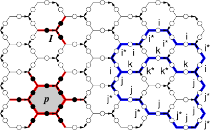
Figure 8: A picture of the lattice spin model (10). The electric charge operator $Q_{\boldsymbol{I}}$ acts on the three spins adjacent to the vertex $\boldsymbol{I}$, while the magnetic energy operator $B_{\boldsymbol{p}}$ acts on the $12$ spins adjacent to the hexagonal plaquette $\boldsymbol{p}$. The term $Q_{\boldsymbol{I}}$ constrains the string-nets to obey the branching rules, while $B_{\boldsymbol{p}}$ provides dynamics. A typical state satisfying the low-energy constraints is shown on the right. The empty links have spins in the $i=0$ state.

The exactly soluble Hamiltonian for our model is given by

$$H=-\sum_{\boldsymbol{I}}Q_{\boldsymbol{I}}-\sum_{\boldsymbol{p}}B_{\boldsymbol{p}},\ \ \ \ \ B_{\boldsymbol{p}}=\sum_{s=0}^{N}a_{s}B_{\boldsymbol{p}}^{s}$$ (10)

where the sums run over vertices $\boldsymbol{I}$ and plaquettes $\boldsymbol{p}$ of the honeycomb lattice. The coefficients $a_{s}$ satisfy $a_{s^{*}}=a_{s}^{*}$ but are otherwise arbitrary.

Let us explain the terms in (10). We think of the first term $Q_{\boldsymbol{I}}$ as an electric charge operator. It measures the “electric charge” at site $\boldsymbol{I}$, and favors states with no charge. It acts on the $3$ spins adjacent to the site $\boldsymbol{I}$:

$$Q_{\boldsymbol{I}}\left|\begin{matrix}\includegraphics[height=21.68121pt]{starD.eps}\end{matrix}\right\rangle=\delta_{ijk}\left|\begin{matrix}\includegraphics[height=21.68121pt]{starD.eps}\end{matrix}\right\rangle$$ (11)

where $\delta_{ijk}$ is the branching rule symbol (9). Clearly, this term constrains the strings to obey the branching rules described by $\delta_{ijk}$. With this constraint the low energy Hilbert space is essentially the set of all allowed string-net configurations on a honeycomb lattice. (See Fig. 8).

We think of the second term $B_{\boldsymbol{p}}$ as a magnetic flux operator. It measures the “magnetic flux” though the plaquette $\boldsymbol{p}$ (or more precisely, the cosine of the magnetic flux) and favors states with no flux. This term provides dynamics for the string-net configurations.

The magnetic flux operator $B_{\boldsymbol{p}}$ is a linear combination of $(N+1)$ terms $B_{\boldsymbol{p}}^{s}$, $s=0,1,...,N$. Each $B_{\boldsymbol{p}}^{s}$ is an operator that acts on the $12$ links that are adjacent to vertices of the hexagon $\boldsymbol{p}$. (See Fig. 8). Thus, the $B_{\boldsymbol{p}}^{s}$ are essentially $(N+1)^{12}\times(N+1)^{12}$ matrices. However, the action of $B_{\boldsymbol{p}}^{s}$ does not change the spin states on the $6$ outer links of $\boldsymbol{p}$. Therefore the $B_{\boldsymbol{p}}^{s}$ can be block diagonalized into $(N+1)^{6}$ blocks, each of dimension $(N+1)^{6}\times(N+1)^{6}$. Let $B^{s,g^{\prime}h^{\prime}i^{\prime}j^{\prime}k^{\prime}l^{\prime}}_{\boldsymbol{p},ghijkl}(abcdef)$, with $a,b,c...=0,1,...,N$, denote the matrix elements of these $(N+1)^{6}$ matrices:

$$B^{s}_{\boldsymbol{p}}\left|\begin{matrix}\includegraphics[height=43.36243pt]{hexstar1O.eps}\end{matrix}\right\rangle$$

$$= \sum_{m,...,r}B_{\boldsymbol{p},ghijkl}^{s,g^{\prime}h^{\prime}i^{\prime}j^{\prime}k^{\prime}l^{\prime}}(abcdef)\left|\begin{matrix}\includegraphics[height=43.36243pt]{hexstar2O.eps}\end{matrix}\right\rangle$$ (12)

Then the operators $B_{\boldsymbol{p}}^{s}$ are defined by

$$B_{\boldsymbol{p},ghijkl}^{s,g^{\prime}h^{\prime}i^{\prime}j^{\prime}k^{\prime}l^{\prime}}(abcdef)$$

$$= \;F^{al^{*}g}_{s^{*}g^{\prime}l^{\prime*}}F^{bg^{*}h}_{s^{*}h^{\prime}g^{\prime*}}F^{ch^{*}i}_{s^{*}i^{\prime}h^{\prime*}}F^{di^{*}j}_{s^{*}j^{\prime}i^{\prime*}}F^{ej^{*}k}_{s^{*}k^{\prime}j^{\prime*}}F^{fk^{*}l}_{s^{*}l^{\prime}k^{\prime*}}$$ (13)

(See appendix C for a graphical representation of $B_{\boldsymbol{p}}^{s}$). One can check that the Hamiltonian (10) is Hermitian if $F$ satisfies

$$F^{i^{*}j^{*}m^{*}}_{k^{*}l^{*}n^{*}}=(F^{ijm}_{kln})^{*}$$ (14)

in addition to (8). Our model is only applicable to topological phases satisfying this additional constraint. We believe that this is true much more generally: only topological phases satisfying the unitarity condition (14) are physically realizable.

The Hamiltonian (10) has a number of interesting properties, provided that $(F^{ijm}_{kln}$, $d_{i})$ satisfy the self-consistency conditions (8). It turns out that:

1. The $B_{\boldsymbol{p}}^{s}$ and $Q_{\boldsymbol{I}}$’s all commute with each other. Thus the Hamiltonian (10) is exactly soluble.

2. Depending on the choice of the coefficients $a_{s}$, the system can be in $N+1$ different quantum phases.

3. The choice $a_{s}=\frac{d_{s}}{\sum_{i=0}^{N}d_{i}^{2}}$ corresponds to a topological phase with a smooth continuum limit. The ground state wave function for this parameter choice is topologically invariant, and obeys the local rules (4-7). It is precisely the wave function $\Phi$, defined on a honeycomb lattice. Furthermore, $Q_{\boldsymbol{I}}$, $B_{\boldsymbol{p}}$ are projection operators in this case. Thus, the ground state satisfies $Q_{\boldsymbol{I}}=B_{\boldsymbol{p}}=1$ for all $\boldsymbol{I}$, $\boldsymbol{p}$, while the excited states violate these constraints.

The Hamiltonian (10) with the above choice of $a_{s}$ provides an exactly soluble realization of the doubled topological phase described by $F^{ijm}_{kln}$. We can obtain some intuition for the Hamiltonian (10) by considering the case where $F^{ijm}_{kln}$ is the $6j$ symbol of some group $G$. In this case, it turns out that $Q_{\boldsymbol{I}}$ and $B_{\boldsymbol{p}}$ are precisely the electric charge and magnetic flux operators in the standard lattice gauge theory with group $G$. Thus, (10) is the usual Hamiltonian of lattice gauge theory, except with no electric field term. This is nothing more than the well-known exactly soluble Hamiltonian of lattice gauge theory. Wegner (1971); Kitaev (2003) In this way, our construction can be viewed as a natural generalization of lattice gauge theory.

In this paper, we will focus on the smooth topological phase corresponding to the parameter choice $a_{s}=\frac{d_{s}}{\sum_{i=0}^{N}d_{i}^{2}}$ (see appendix C). However, we would like to mention that the other $N$ quantum phases also have non-trivial topological (or quantum) order. However, in these phases, the ground state wave function does not have a smooth continuum limit. Thus, these are new topological phases beyond those described by continuum theories.

IV.3 Quasiparticle excitations

In this section, we find the quasiparticle excitations of the string-net Hamiltonian (10), and calculate their statistics (e.g. the twists $\theta_{\alpha}$ and the $S$ matrix $s_{\alpha\beta}$). We will only consider the topological phase with smooth continuum limit. That is, we will choose $a_{s}=\frac{d_{s}}{\sum_{i=0}^{N}d_{i}^{2}}$ in our lattice model.

Recall that the ground state satisfies $Q_{\boldsymbol{I}}=B_{\boldsymbol{p}}=1$ for all vertices $\boldsymbol{I}$, and all plaquettes $\boldsymbol{p}$. The quasiparticle excitations correspond to violations of these constraints for some local collection of vertices and plaquettes. We are interested in the topological properties (e.g. statistics) of these excitations.

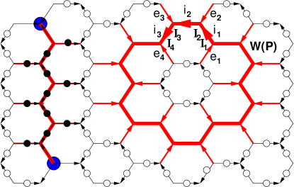
Figure 9: Open and closed string operators for the lattice spin model (10). Open string operators create quasiparticles at the two ends, as shown on the left. Closed string operators, as shown on the right, commute with the Hamiltonian. The closed string operator $W(P)$ only acts non-trivially on the spins along the path $P=\boldsymbol{I_{1}},\boldsymbol{I_{2}}...$ (thick line), but its action depends on the spin states on the legs (thin lines). The matrix element between an initial state $i_{1},i_{2},...$ and a final state $i^{\prime}_{1},i^{\prime}_{2},...$ is $W_{i_{1}i_{2}...}^{i^{\prime}_{1}i^{\prime}_{2}...}(e_{1}e_{2}...)=(F^{e_{2}i^{*}_{2}i_{1}}_{s^{*}i^{\prime}_{1}i_{2}^{\prime*}}F^{e_{3}i^{*}_{3}i_{2}}_{s^{*}i^{\prime}_{2}i_{3}^{\prime*}}...)\cdot(\frac{v_{i_{1}}v_{s_{1}}}{v_{i_{1}^{\prime}}}\omega^{i^{\prime}_{1}}_{i_{1}}\frac{v_{i_{3}}v_{s_{3}}}{v_{i_{3}^{\prime}}}\bar{\omega}^{i^{\prime}_{3}}_{i_{3}}...)$ for a type-$s$ simple string and $W_{i_{1}i_{2}...}^{i^{\prime}_{1}i^{\prime}_{2}...}(e_{1}e_{2}...)=\sum_{\{s_{k}\}}(F^{e_{2}i^{*}_{2}i_{1}}_{s^{*}_{2}i^{\prime}_{1}i_{2}^{\prime*}}F^{e_{3}i^{*}_{3}i_{2}}_{s^{*}_{3}i^{\prime}_{2}i_{3}^{\prime*}}...)\cdot{\rm Tr}(\frac{v_{i_{1}}v_{s_{1}}}{v_{i_{1}^{\prime}}}\Omega^{i^{\prime}_{1}}_{s_{1}s_{2}i_{1}}\delta_{s_{2}s_{3}}\text{Id}\frac{v_{i_{3}}v_{s_{3}}}{v_{i_{3}^{\prime}}}\bar{\Omega}^{i^{\prime}_{3}}_{s_{3}s_{4}i_{3}}...)$ for a general string.

We will focus on topologically nontrivial quasiparticles - that is, particles with nontrivial statistics or mutual statistics. By the analysis in LABEL:LWsta, we know that these types of particles are always created in pairs, and that their pair creation operator has a string-like structure, with the newly created particles appearing at the ends. (See Fig. 9). The position of this string operator is unobservable in the string-net condensed state - only the endpoints of the string are observable. Thus the two ends of the string behave like independent particles.

If the two endpoints of the string coincide so that the string forms a loop, then the associated closed string operator commutes with the Hamiltonian. This follows from the fact that the string is truly unobservable; the action of an open string operator on the ground state depends only on its endpoints.

Thus, each topologically nontrivial quasiparticle is associated with a (closed) string operator that commutes with the Hamiltonian. To find the quasiparticles, we need to find these closed string operators.

An important class of string operators are what we will call “simple” string operators. The defining property of simple string operators is their action on the vacuum state. If we apply a type-$s$ simple string operator $W(P)$ to the vacuum state, it creates a type-$s$ string along the path of the string, $P$. We already have some examples of these operators, namely the magnetic flux operators $B^{s}_{\boldsymbol{p}}$. When $B^{s}_{\boldsymbol{p}}$ acts on the vacuum configuration $|0\rangle$, it creates a type-$s$ string along the boundary of the plaquette $\boldsymbol{p}$. Thus, we can think of $B^{s}_{\boldsymbol{p}}$ as a short type-$s$ simple string operator, $W(\partial\boldsymbol{p})$.

We would like to construct simple string operators $W(P)$ for arbitrary paths $P=\boldsymbol{I_{1}},...,\boldsymbol{I_{N}}$ on the honeycomb lattice. Using the definition of $B^{s}_{\boldsymbol{p}}$ as a guide, we make the following ansatz. The string operator $W(P)$ only changes the spin states along the path $P$. The matrix element of a general type-$s$ simple string operator $W(P)$ between an initial spin state $i_{1},...i_{N}$ and final spin state $i^{\prime}_{1},...i^{\prime}_{N}$ is of the form

$$W_{i_{1}i_{2}...i_{N}}^{i_{1}^{\prime}i_{2}^{\prime}...i_{N}^{\prime}}(e_{1}e_{2}...e_{N})=\left(\prod_{k=1}^{N}F^{s}_{k}\right)\left(\prod_{k=1}^{N}\omega_{k}\right)$$ (15)

where $e_{1},...,e_{N}$ are the spin states of the $N$ “legs” of $P$ (see Fig. 9) and

$$F^{s}_{k}=\left\{\begin{matrix}F^{e_{k}i_{k}^{*}i_{k-1}}_{s^{*}i_{k-1}^{\prime}i_{k}^{\prime*}},&\text{if $P$ turns left at $\boldsymbol{I_{k}}$}\\ F^{e_{k}i_{k-1}^{*}i_{k}}_{si_{k}^{\prime}i_{k-1}^{\prime*}},&\text{if $P$ turns right at $\boldsymbol{I_{k}}$}\end{matrix}\right.$$ (16)

$$\omega_{k}=\left\{\begin{matrix}\frac{v_{i_{k}}v_{s}}{v_{i_{k}^{\prime}}}\omega^{i_{k}^{\prime}}_{i_{k}},&\text{if $P$ turns right, left at $\boldsymbol{I_{k}}$, $\boldsymbol{I_{k+1}}$}\\ \frac{v_{i_{k}}v_{s}}{v_{i_{k}^{\prime}}}\bar{\omega}^{i_{k}^{\prime}}_{i_{k}},&\text{if $P$ turns left, right at $\boldsymbol{I_{k}}$, $\boldsymbol{I_{k+1}}$}\\ $1$,&\text{otherwise}\end{matrix}\right.$$ (17)

Here, $\omega^{i}_{j}$, $\bar{\omega}^{i}_{j}$ are two (complex) two index objects that characterize the string $W$.

Note the similarity to the definition of $B^{s}_{\boldsymbol{p}}$. The major difference is the additional factor $\prod_{k=1}^{N}\omega_{k}$. We conjecture that $|\omega^{j}_{i}\frac{v_{i}v_{s}}{v_{j}}|=1$ for a type-$s$ string, so $\prod_{k=1}^{N}\omega_{k}$ is simply a phase factor that depends on the initial and final spin states $i_{1}$, $i_{2}$, …, $i_{N}$, $i^{\prime}_{1}$, $i^{\prime}_{2}$, …, $i^{\prime}_{N}$. This phase vanishes for paths $P$ that make only left or only right turns, such as plaquette boundaries $\partial\boldsymbol{p}$. In that case, the definition of $W(P)$ coincides with $B^{s}_{\boldsymbol{p}}$.

A straightforward calculation shows that the operator $W(P)$ defined above commutes with the Hamiltonian (10) if $\omega^{i}_{j},\bar{\omega}^{i}_{j}$ satisfy

$$\bar{\omega}^{m}_{j}F^{sl^{*}i}_{kjm^{*}}\omega^{l}_{i}\frac{v_{j}v_{s}}{v_{m}} = \sum_{n=0}^{N}F^{ji^{*}k}_{s^{*}nl^{*}}\omega^{n}_{k}F^{jl^{*}n}_{ksm^{*}}$$

$$\bar{\omega}^{j}_{i} = \sum_{k=0}^{N}\omega^{k}_{i^{*}}F^{is^{*}k}_{i^{*}sj*}$$ (18)

The solutions to these equations give all the type-$s$ simple string operators.

For example, consider the case of Abelian gauge theory. In this case, the solutions to (IV.3) can be divided into three classes. The first class is given by $s\neq 0$, $\omega^{j}_{i}\frac{v_{i}v_{s}}{v_{j}}=\bar{\omega}^{j}_{i}\frac{v_{i}v_{s}}{v_{j}}=1$. These string operators create electric flux lines and the associated quasiparticles are electric charges. In more traditional nomenclature, these are known as (Wegner-)Wilson loop operators Wegner (1971); Wilson (1974). The second class of solutions is given by $s=0$, and $\omega^{j}_{i}\frac{v_{i}v_{s}}{v_{j}}=(\bar{\omega}^{j}_{i}\frac{v_{i}v_{s}}{v_{j}})^{*}\neq 1$. These string operators create magnetic flux lines and the associated quasiparticles are magnetic fluxes. The third class has $s\neq 0$ and $\omega^{j}_{i}\frac{v_{i}v_{s}}{v_{j}}=(\bar{\omega}^{j}_{i}\frac{v_{i}v_{s}}{v_{j}})^{*}\neq 1$. These strings create both electric and magnetic flux and the associated quasiparticles are electric charge/magnetic flux bound states. This accounts for all the quasiparticles in $(2+1)D$ Abelian gauge theory. Therefore, all the string operators are simple in this case.

However, this is not true for non-Abelian gauge theory or other $(2+1)D$ topological phases. To compute the quasiparticle spectrum of these more general theories, we need to generalize the expression (15) for $W(P)$ to include string operators that are not simple.

One way to guess the more general expression for $W(P)$ is to consider products of simple string operators. Clearly, if $W_{1}(P)$ and $W_{2}(P)$ commute with the Hamiltonian, then $W(P)=W_{1}(P)\cdot W_{2}(P)$ also commutes with the Hamiltonian. Thus, we can obtain other string operators by taking products of simple string operators. In general, the resulting operators are not simple. If $W_{1}$ and $W_{2}$ are type-$s_{1}$ and type-$s_{2}$ simple string operators, then the action of the product string on the vacuum state is:

$$W(P)|0\rangle=W_{1}(P)W_{2}(P)|0\rangle=W_{1}(P)|s_{2}\rangle=\sum_{s}\delta_{ss_{1}s_{2}}|s\rangle$$

where $|s\rangle$ denotes the string state with a type-$s$ string along the path $P$ and the vacuum everywhere else. If we take products of more then two simple string operators then the action of the product string on the vacuum is of the form $W(P)|0\rangle=\sum_{s}n_{s}|s\rangle$ where $n_{s}$ are some non-negative integers.

We now generalize the expression for $W(P)$ so that it includes arbitrary products of simple strings. Let $W$ be a product of simple string operators, and let $n_{s}$ be the non-negative integers characterizing the action of $W$ on the vacuum: $W(P)|0\rangle=\sum_{s}n_{s}|s\rangle$. Then, one can show that the matrix elements of $W(P)$ are always of the form

$$W_{i_{1}i_{2}...i_{N}}^{i_{1}^{\prime}i_{2}^{\prime}...i_{N}^{\prime}}(e_{1}e_{2}...e_{N})=\sum_{\{s_{k}\}}\left(\prod_{k=1}^{N}F^{s_{k}}_{k}\right){\rm Tr}\left(\prod_{k=1}^{N}\Omega^{s_{k}}_{k}\right)$$ (19)

where

$$\Omega^{s_{k}}_{k}=\left\{\begin{matrix}\frac{v_{i_{k}}v_{s_{k}}}{v_{i_{k}^{\prime}}}\Omega^{i_{k}^{\prime}}_{s_{k}s_{k+1}i_{k}},&\text{if $P$ turns right, left at $\boldsymbol{I_{k}}$, $\boldsymbol{I_{k+1}}$}\\ \frac{v_{i_{k}}v_{s_{k}}}{v_{i_{k}^{\prime}}}\bar{\Omega}^{i_{k}^{\prime}}_{s_{k}s_{k+1}i_{k}},&\text{if $P$ turns left, right at $\boldsymbol{I_{k}}$, $\boldsymbol{I_{k+1}}$}\\ \delta_{s_{k}s_{k+1}}\cdot\text{Id},&\text{otherwise}\end{matrix}\right.$$ (20)

and $\Omega^{i}_{stj}$,$\bar{\Omega}^{i}_{stj}$ are two $4$ index objects that characterize the string operator $W$. For any quadruple of string types $i,j,s,t$, $(\Omega^{i}_{stj}$, $\bar{\Omega}^{i}_{stj})$ are (complex) rectangular matrices of dimension $n_{s}\times n_{t}$. Note that type-$s_{0}$ simple string operators correspond to the special case where $n_{s}=\delta_{s_{0}s}$. In this case, the matrices $\Omega^{i}_{stj},\bar{\Omega}^{i}_{stj}$ reduce to complex numbers, and we can identify

$$\Omega^{i}_{stj}=\omega^{i}_{j}\delta_{ss_{0}}\delta_{ts_{0}},\ \ \ \ \ \ \ \ \ \bar{\Omega}^{i}_{stj}=\bar{\omega}^{i}_{j}\delta_{ss_{0}}\delta_{ts_{0}}.$$ (21)

As we mentioned above, products of simple string operators are always of the form (19). In fact, we believe that all string operators are of this form. Thus, we will use (19) as an ansatz for general string operators in $(2+1)D$ topological phases. This ansatz is complicated algebraically, but like the definition of $B^{s}_{\boldsymbol{p}}$, it has a simple graphical interpretation (see appendix D).

A straightforward calculation shows that the closed string $W(P)$ commutes with the Hamiltonian (10) if $\Omega$ and $\bar{\Omega}$ satisfy

$$\sum_{s=0}^{N}\bar{\Omega}^{m}_{rsj}F^{sl^{*}i}_{kjm^{*}}\Omega^{l}_{sti}\frac{v_{j}v_{s}}{v_{m}} = \sum_{n=0}^{N}F^{ji^{*}k}_{t^{*}nl^{*}}\Omega^{n}_{rtk}F^{jl^{*}n}_{krm^{*}}$$

$$\bar{\Omega}^{j}_{sti} = \sum_{k=0}^{N}\Omega^{k}_{sti^{*}}F^{it^{*}k}_{i^{*}sj*}$$ (22)

The solutions $(\Omega_{m},\bar{\Omega}_{m})$ to these equations give all the different closed string operators $W_{m}$. However, not all of these solutions are really distinct. Notice that two solutions $(\Omega_{1},\bar{\Omega}_{1})$, $(\Omega_{2},\bar{\Omega}_{2})$ can be combined to form a new solution $(\Omega^{\prime},\bar{\Omega}^{\prime})$:

$$\Omega^{\prime j}_{sti}=\Omega^{j}_{1,sti}\oplus\Omega^{j}_{2,sti}$$

$$\bar{\Omega}^{\prime j}_{sti}=\bar{\Omega}^{j}_{1,sti}\oplus\bar{\Omega}^{j}_{2,sti}$$ (23)

This is not surprising: the string operator $W^{\prime}$ corresponding to $(\Omega^{\prime},\bar{\Omega}^{\prime})$ is simply the sum of the two operators corresponding to $(\Omega_{1,2},\bar{\Omega}_{1,2})$: $W^{\prime}=W_{1}+W_{2}$.

Given this additivity property, it is natural to consider the “irreducible” solutions $(\Omega_{\alpha},\bar{\Omega}_{\alpha})$ that cannot be written as a sum of two other solutions. Only the “irreducible” string operators $W_{\alpha}$ create quasiparticle-pairs in the usual sense. Reducible string operators $W$ create superpositions of different strings - which correspond to superpositions of different quasiparticles.

To analyze a topological phase, one only needs to find the irreducible solutions $(\Omega_{\alpha},\bar{\Omega}_{\alpha})$ to (IV.3). The number $M$ of such solutions is always finite. In general, each solution corresponds to an irreducible representation of an algebraic object. In the case of lattice gauge theory, there is one solution for every irreducible representation of the quantum double $D(G)$ of the gauge group $G$. Similarly, in the case of doubled Chern-Simons theories there is one solution for each irreducible representation of a doubled quantum group.

The structure of these irreducible string operators $W_{\alpha}$ determines all the universal features of the topological phase. The number $M$ of irreducible string operators is the number of different kinds of quasiparticles. The fusion rules $W_{\alpha}W_{\beta}=\sum_{\gamma=1}^{M}h_{\alpha\beta}^{\gamma}W_{\gamma}$ determine how bound states of type-$\alpha$ and type-$\beta$ quasiparticles can be viewed as a superposition of other types of quasiparticles.

The topological properties of the quasiparticles are also easy to compute. As an example, we now derive two particularly fundamental objects that characterize the spins and statistics of quasiparticles: the $M$ twists $\theta_{\alpha}$ and the $M\times M$ S-matrix, $s_{\alpha\beta}$ Verlinde (1988); Witten (1989a, b); Wen (1990).

The twists $\theta_{\alpha}$ are defined to be statistical angles of the type-$\alpha$ quasiparticles. By the spin-statistics theorem they are closely connected to the quasiparticle spins $s_{\alpha}$: $e^{i\theta_{\alpha}}=e^{2\pi is_{\alpha}}$. We can calculate $\theta_{\alpha}$ by comparing the quantum mechanical amplitude for the following two processes. In the first process, we create a pair of quasiparticles $\alpha,\bar{\alpha}$ (from the ground state), exchange them, and then annihilate the pair. In the second process, we create and then annihilate the pair without any exchange. The ratio of the amplitudes for these two processes is precisely $e^{i\theta_{\alpha}}$.

The amplitude for each process is given by the expectation value of the closed string operator $W_{\alpha}$ for a particular path $P$:

$$\mathcal{A}_{1} = \Big{\langle}\Phi\Big{|}\begin{matrix}\includegraphics[height=21.68121pt]{twst.eps}\end{matrix}\Big{|}\Phi\Big{\rangle}$$ (24)

$$\mathcal{A}_{2} = \Big{\langle}\Phi\Big{|}\begin{matrix}\includegraphics[height=21.68121pt]{untwst.eps}\end{matrix}\Big{|}\Phi\Big{\rangle}$$ (25)

Here, $|\Phi\rangle$ denotes the ground state of the Hamiltonian (10).

Let $(\Omega_{\alpha},\bar{\Omega}_{\alpha},n_{\alpha})$ be the irreducible solution corresponding to the string operator $W_{\alpha}$. The above two amplitudes can be then be expressed in terms of $(\Omega_{\alpha},\bar{\Omega}_{\alpha},n_{\alpha})$ (see appendix D):

$$\mathcal{A}_{1} = \sum_{s}d_{s}^{2}\cdot{\rm Tr}(\Omega^{0}_{\alpha,sss^{*}})$$ (26)

$$\mathcal{A}_{2} = \sum_{s}n_{\alpha,s}d_{s}$$ (27)

Combining these results, we find that the twists are given by

$$e^{i\theta_{\alpha}}=\frac{\mathcal{A}_{1}}{\mathcal{A}_{2}}=\frac{\sum_{s}d_{s}^{2}\cdot{\rm Tr}(\Omega^{0}_{\alpha,sss^{*}})}{\sum_{s}n_{\alpha,s}d_{s}}$$ (28)

Just as the twists $\theta_{\alpha}$ are related to the spin and statistics of individual particle types $\alpha$, the elements of the S-matrix, $s_{\alpha\beta}$ describe the mutual statistics of two particle types $\alpha,\beta$. Consider the following process: We create two pairs of quasiparticles $\alpha,\bar{\alpha},\beta,\bar{\beta}$, braid $\alpha$ around $\beta$, and then annihilate the two pairs. The element $s_{\alpha\beta}$ is defined to be the quantum mechanical amplitude $\mathcal{A}$ of this process, divided by a proportionality factor $D$ where $D^{2}=\sum_{\alpha}(\sum_{s}n_{\alpha,s}d_{s})^{2}$. The amplitude $\mathcal{A}$ can be calculated from the expectation value of $W_{\alpha},W_{\beta}$ for two “linked” paths $P$:

$$\mathcal{A}=\Big{\langle}\Phi\Big{|}\begin{matrix}\includegraphics[height=21.68121pt]{link.eps}\end{matrix}\Big{|}\Phi\Big{\rangle}$$ (29)

Expressing $\mathcal{A}$ in terms of $(\Omega_{\alpha},\bar{\Omega}_{\alpha},n_{\alpha})$, we find

$$s_{\alpha\beta}=\frac{\mathcal{A}}{D}=\frac{1}{D}\sum_{ijk}{\rm Tr}(\Omega^{k}_{\alpha,iij^{*}})\cdot{\rm Tr}(\Omega^{k^{*}}_{\beta,jji^{*}})d_{i}d_{j}$$ (30)

V String-net condensation in $(3+1)$ and higher dimensions

In this section, we generalize our results to $(3+1)$ and higher dimensions. We find that there is a one-to-one correspondence between $(3+1)$ (and higher) dimensional string-net condensates and mathematical objects known as “symmetric tensor categories.” Kassel (1995) The low energy effective theories for these states are gauge theories coupled to bosonic or fermionic charges.

Our approach is based on the exactly soluble lattice spin Hamiltonian (10). In that model, the spins live on the links of the honeycomb lattice. However, the choice of lattice was somewhat arbitrary: we could equally well have chosen any trivalent lattice in two dimensions.

Trivalent lattices can also be constructed in three and higher dimensions. For example, we can create a space-filling trivalent lattice in three dimensions, by “splitting” the sites of the cubic lattice (see Fig. 10). Consider the spin Hamiltonian (10) for this lattice, where $\boldsymbol{I}$ runs over all the vertices of the lattice, and $\boldsymbol{p}$ runs over all the “plaquettes” (that is, the closed loops that correspond to plaquettes in the original cubic lattice).

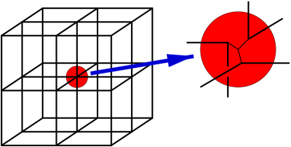
Figure 10: A three dimensional trivalent lattice, obtained by splitting the sites of the cubic lattice. We replace each vertex of the cubic lattice with $4$ other vertices as shown above.

This model is a natural candidate for string-net condensation in three dimensions. Unfortunately, it turns out that the Hamiltonian (10) is not exactly soluble on this lattice. The magnetic flux operators $B^{s}_{\boldsymbol{p}}$ do not commute in general.

This lack of commutativity originates from two differences between the plaquettes in the honeycomb lattice and in higher dimensional trivalent lattices. The first difference is that in the honeycomb lattice, neighboring plaquettes always share precisely two vertices, while in higher dimensions the boundary between plaquettes can contain three or more vertices (see Fig. 11). The existence of these interior vertices has the following consequence. Imagine we choose orientation conventions for each vertex, so that we have a notion of “left turns” and “right turns” for oriented paths on our lattice (such an orientation convention can be obtained by projecting the $3D$ lattice onto a $2D$ plane - as in Fig. 11). Then, no matter how we assign these orientations the plaquette boundaries will always make both left and right turns. Thus, we cannot regard the boundaries of the $3D$ plaquettes as small closed strings the way we did in two dimensions (since small closed strings always make all left turns, or all right turns). But the magnetic flux operators $B^{s}_{\boldsymbol{p}}$ only commute if their boundaries are small closed strings. It is this inconsistency between the algebraic definition of $B^{s}_{\boldsymbol{p}}$ and the topology of the plaquettes that leads to the lack of commutativity.

To resolve this problem, we need to define a Hamiltonian using the general simple string operators $W(\partial\boldsymbol{p})$ rather then the small closed strings $B^{s}_{\boldsymbol{p}}$. Suppose $(\omega^{i}_{sj},\bar{\omega}^{i}_{sj})$, $s=0,1,...N$ are type-$s$ solutions of (IV.3). After picking some “left turn”, “right turn” orientation convention at each vertex, we can define the corresponding type-$s$ simple string operators $W_{s}(P)$ as in (15). Suppose, in addition, that we choose $(\omega^{i}_{sj},\bar{\omega}^{i}_{sj})$ so that the string operators satisfy $W_{r}\cdot W_{s}=\sum_{t}\delta_{rst}W_{t}$ (this property ensures that $W_{s}(\partial\boldsymbol{p})$ are analogous to $B^{s}_{\boldsymbol{p}}$). Then, a natural higher dimensional generalization of the Hamiltonian (10) is

$$H=-\sum_{\boldsymbol{I}}Q_{\boldsymbol{I}}-\sum_{\boldsymbol{p}}W_{\boldsymbol{p}},\ \ \ \ \ W_{\boldsymbol{p}}=\sum_{s=0}^{N}a_{s}W_{s}(\partial\boldsymbol{p})$$ (31)

For a two dimensional lattice, the conditions (IV.3) are sufficient to guarantee that the Hamiltonian (31) is an exactly soluble realization of a doubled topological phase. (This is because the plaquette boundaries $\partial\boldsymbol{p}$ are not linked and hence the $W_{s}(\partial\boldsymbol{p})$ all commute). However, in higher dimensions, one additional constraint is necessary.

Figure 11: Three plaquettes demonstrating the two fundamental differences between higher dimensional trivalent lattices and the honeycomb lattice. The plaquettes $\boldsymbol{p_{1}}$, $\boldsymbol{p_{2}}$ lie in the $xz$ plane, while $\boldsymbol{p_{3}}$ is oriented in the $xy$ direction. Notice that $\boldsymbol{p_{1}}$ and $\boldsymbol{p_{2}}$ share three vertices, $\boldsymbol{I_{1}}$, $\boldsymbol{I_{2}}$, $\boldsymbol{I_{3}}$. Also, notice that the plaquette boundaries $\partial\boldsymbol{p_{1}}$ and $\partial\boldsymbol{p_{3}}$ intersect only at the line segment $\boldsymbol{I_{3}}\boldsymbol{I_{4}}$. The boundary $\partial\boldsymbol{p_{1}}$ makes a left turn at $\boldsymbol{I_{3}}$, and a right turn at $\boldsymbol{I_{4}}$. Thus, viewed from far away, these two plaquette boundaries intersect exactly once (unlike the pair $\partial\boldsymbol{p_{1}}$ and $\partial\boldsymbol{p_{2}}$).

This constraint stems from the second, and perhaps more fundamental, difference between $2D$ and higher dimensional lattices. In two dimensions, two closed curves always intersect an even number of times. For higher dimensional lattices, this is not the case. Small closed curves, in particular plaquette boundaries, can (in a sense) intersect exactly once (see Fig. 11). Because of this, the objects $\omega^{i}_{jk}$ must satisfy the additional relation:

$$\omega^{i}_{jk}=\bar{\omega}^{i}_{kj}$$ (32)

One can show that if this additional constraint is satisfied, then (a) the higher dimensional Hamiltonian (31) is exactly soluble, and (b) the ground state wave function $\Phi$ is defined by local topological rules analogous to (4-7). This means that (31) provides an exactly soluble realization of topological phases in $(3+1)$ and higher dimensions.

Each exactly soluble Hamiltonian is associated with a solution $(F^{ijm}_{kln},\omega^{i}_{jk},\bar{\omega}^{i}_{jk})$ of (8), (IV.3), (32). By analogy with the two dimensional case, we conjecture that there is a one-to-one correspondence between topological string-net condensed phases in $(3+1)$ or higher dimensions, and these solutions. The solutions $(F^{ijm}_{kln},\omega^{i}_{jk},\bar{\omega}^{i}_{jk})$ correspond to a special class of tensor categories - symmetric tensor categories. Kassel (1995) Thus, just as tensor categories are the mathematical objects underlying string condensation in $(2+1)$ dimensions, symmetric tensor categories are fundamental to string condensation in higher dimensions.

There are relatively few solutions to (8), (IV.3), (32). Physically, this is a consequence of the restrictions on quasiparticle statistics in $3$ or higher dimensions. Unlike in two dimensions, higher dimensional quasiparticles necessarily have trivial mutual statistics, and must be either bosonic or fermionic. From a more mathematical point of view, the scarcity of solutions is a result of the symmetry condition (32). Doubled topological phases, such as Chern-Simons theories, typically fail to satisfy this condition.

However, gauge theories do satisfy the symmetry condition (32) and therefore do correspond to higher dimensional string-net condensates. Recall that the gauge theory solution to (8) is obtained by (a) letting the string-type index $i$ run over the irreducible representations of the gauge group, (b) letting the numbers $d_{i}$ be the dimensions of the representations, and (c) letting the $6$ index object $F^{ijm}_{kln}$ be the $6j$ symbol of the group. One can check that this also provides a solution to (IV.3), (32), if we set $\omega^{i}_{jk}\frac{v_{j}v_{k}}{v_{i}}=-1$ when $j=k$ and the invariant tensor in $k\otimes k\otimes i^{*}$ is antisymmetric in the first two indices, and $\omega^{i}_{jk}\frac{v_{j}v_{k}}{v_{i}}=1$ otherwise. This result is to be expected, since the string-net picture of gauge theory (section II) is valid in any number of dimensions. Thus, it is not surprising that gauge theories can emerge from higher dimensional string-net condensation.

There is another class of higher dimensional string-net condensed phases that is more interesting. The low energy effective theories for these phases are variants of gauge theories. Mathematically, they are obtained by twisting the usual gauge theory solution by

$$\tilde{\omega}^{i}_{jk}=\omega^{i}_{jk}\cdot(-1)^{P(j)P(k)}$$ (33)

Here $P(i)$ is some assignment of parity (“even”, or “odd”) to each representation $i$. The assignment must be self-consistent in the sense that the tensor product of two representations with the same (different) parity, decomposes into purely even (odd) representations. If all the representations are assigned an even parity - that is $P(i)$ is trivial - then the twisted gauge theory reduces to standard gauge theory.

The major physical distinction between twisted gauge theories and standard gauge theories is the quasiparticle spectrum. In standard gauge theory, the fundamental quasiparticles are the electric charges created by the $N+1$ string operators $W_{i}$. These quasiparticles are all bosonic. In contrast, in twisted gauge theories, all the quasiparticles corresponding to “odd” representations $i$ are fermionic.

In this way, higher dimensional string-net condensation naturally gives rise to both emerging gauge bosons and emerging fermions. This feature suggests that gauge interactions and Fermi statistics may be intimately connected. The string-net picture may be the bridge between these two seemingly unrelated phenomena. Levin and Wen (2003)

In fact, it appears that gauge theories coupled to fermionic or bosonic charged particles are the only possibilities for higher dimensional string-net condensates: mathematical work on symmetric tensor categories suggests that the only solutions to (8), (IV.3), (32) are those corresponding to gauge theories and twisted gauge theories. Etingof and Gelaki (2003)

We would like to point out that $(3+1)$ dimensional string-net condensed states also exhibit membrane condensation. These membrane operators are entirely analogous to the string operators. Just as open string operators create charges at their two ends, open membrane operators create magnetic flux loops along their boundaries. Furthermore, just as string condensation makes the string unobservable, membrane condensation leads to the unobservability of the membrane. Only the boundary of the membrane - the magnetic flux loop - is observable.

VI Examples

VI.1 $N=1$ string model

We begin with the simplest string-net model. In the notation from section III, this model is given by

1. Number of string types: $N=1$

2. Branching rules: $\emptyset$ (no branching)

3. String orientations: $1^{*}=1$.

In other words, the string-nets in this model contain one unoriented string type and have no branching. Thus, they are simply closed loops. (See Fig. 3a).

We would like to find the different topological phases that can emerge from these closed loops. According to the discussion in section IV, each phase is captured by a fixed-point wave function, and each fixed-point wave function is specified by local rules (4-7) that satisfy the self-consistency relations (8). It turns out that (8) have only two solutions in this case (up to rescaling):

$$d_{0} = 1$$

$$d_{1} = F^{110}_{110}=\pm 1$$

$$F^{000}_{000} = F^{101}_{101}=F^{011}_{011}=1$$

$$F^{000}_{111} = F^{110}_{001}=F^{101}_{010}=F^{011}_{100}=1$$ (34)

where the other elements of $F$ all vanish. The corresponding local rules (4-7) are:

$$\Phi\begin{pmatrix}\includegraphics[height=16.62178pt]{Xl.eps}\end{pmatrix}= \pm\Phi\begin{pmatrix}\includegraphics[height=16.62178pt]{X0.eps}\end{pmatrix}$$

$$\Phi\begin{pmatrix}\includegraphics[height=16.62178pt]{XijklX.eps}\end{pmatrix}= \pm\Phi\begin{pmatrix}\includegraphics[height=16.62178pt]{XijX.eps}\end{pmatrix}$$ (35)

We have omitted those rules that can be derived from topological invariance (4).

The fixed-point wave functions $\Phi_{\pm}$ satisfying these rules are given by

$$\Phi_{\pm}(X)=(\pm 1)^{X_{c}}$$ (36)

where $X_{c}$ is the number of disconnected components in the string configuration $X$.

The two fixed-point wave functions $\Phi_{\pm}$ correspond to two simple topological phases. As we will see, $\Phi_{+}$ corresponds to $Z_{2}$ gauge theory, while $\Phi_{-}$ is a $U(1)\times U(1)$ Chern-Simons theory. (Actually, other topological phases can emerge from closed loops - such as in LABEL:F0160,FNS0311,FNS0320. However, we regard these phases as emerging from more complicated string-nets. The closed loops organize into these effective string-nets in the infrared limit).

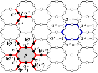
Figure 12: The Hamiltonians (39), (40), realizing the two $N=1$ string-condensed phases. Each circle denotes a spin-1/2 spin. The links with $\sigma^{x}=-1$ are thought of as being occupied by a type-$1$ string, while the links with $\sigma^{x}=+1$ are regarded as empty. The electric charge term acts on the three legs of the vertex $\boldsymbol{I}$ with $\sigma^{x}$. The magnetic energy term acts on the $6$ edges of the plaquette $\boldsymbol{p}$ with $\sigma^{z}$, and acts on the $6$ legs of $\boldsymbol{p}$ with an operator of the form $f(\sigma^{x})$. For the $Z_{2}$ phase, $f=1$, while for the Chern-Simons phase, $f(x)=i^{(1-x)/2}$.

The exactly soluble models (10) realizing these two phases can be written as spin $1/2$ systems with one spin on each link of the honeycomb lattice (see Fig. 12). We regard a link with $\sigma^{x}=-1$ as being occupied by a type-$1$ string, and the state $\sigma^{x}=+1$ as being unoccupied (or equivalently, occupied by a type-$0$ or null string). The Hamiltonians for the two phases are of the form

$$H_{\pm}=-\sum_{\boldsymbol{I}}Q_{\boldsymbol{I},\pm}-\sum_{\boldsymbol{p}}B_{\boldsymbol{p},\pm}$$

The electric charge term is the same for both phases (since it only depends on the branching rules):

$$Q_{\boldsymbol{I},\pm}=\frac{1}{2}(1+\prod_{\text{legs of }\boldsymbol{I}}\sigma_{\boldsymbol{i}}^{x})$$ (37)

The magnetic terms for the two phases are

$$B_{\boldsymbol{p},\pm} = \frac{1}{2}(B_{\boldsymbol{p},\pm}^{0}\pm B_{\boldsymbol{p},\pm}^{1})$$

$$= \frac{1}{2}\left(1\pm\prod_{\text{edges of }\boldsymbol{p}}\sigma^{z}_{\boldsymbol{j}}\cdot\prod_{\text{legs of }\boldsymbol{p}}(\sqrt{\pm 1})^{\frac{1-\sigma^{x}_{\boldsymbol{j}}}{2}}\right)P_{\boldsymbol{p}}$$

where $P_{\boldsymbol{p}}$ is the projection operator $P_{\boldsymbol{p}}=\prod_{\boldsymbol{I}\in\boldsymbol{p}}Q_{\boldsymbol{I}}$. The projection operator $P_{\boldsymbol{p}}$ can be omitted without affecting the physics (or the exact solubility of the Hamiltonian). We have included it only to be consistent with (10). If we omit this term, the Hamiltonian for the first phase ($\Phi_{+}$) reduces to the usual exactly soluble Hamiltonian of $Z_{2}$ lattice gauge theory (neglecting numerical factors):

$$H_{+}=-\sum_{\boldsymbol{I}}\prod_{\text{legs of }\boldsymbol{I}}\sigma_{\boldsymbol{i}}^{x}-\sum_{\boldsymbol{p}}\prod_{\text{edges of }\boldsymbol{p}}\sigma^{z}_{\boldsymbol{j}}$$ (39)

The Hamiltonian for the second phase,

$$H_{-}=-\sum_{\boldsymbol{I}}\prod_{\text{legs of }\boldsymbol{I}}\sigma_{\boldsymbol{i}}^{x}+\sum_{\boldsymbol{p}}(\prod_{\text{edges of }\boldsymbol{p}}\sigma^{z}_{\boldsymbol{j}})(\prod_{\text{legs of }\boldsymbol{p}}i^{\frac{1-\sigma^{x}_{\boldsymbol{j}}}{2}})$$ (40)

is less familiar. However, one can check that in both cases, the Hamiltonians are exactly soluble and the two ground state wave functions are precisely $\Phi_{\pm}$ (in the $\sigma^{x}$ basis).

Next we find the quasiparticle excitations for the two phases, and the corresponding S-matrix and twists $\theta_{\alpha}$.

In both cases, equation (IV.3) has 4 irreducible solutions $(n_{\alpha,s},\Omega^{ij}_{\alpha,st},\bar{\Omega}^{ij}_{\alpha,st})$, $\alpha=1,2,3,4$ - corresponding to 4 quasiparticle types. For the first phase ($\Phi_{+}$) these solutions are given by:

$$\begin{array}[]{llll}n_{1,0}=1,&n_{1,1}=0,&\Omega^{0}_{1,000}=1,&\Omega^{1}_{1,001}=1\\ n_{2,0}=0,&n_{2,1}=1,&\Omega^{1}_{2,110}=1,&\Omega^{0}_{2,111}=1\\ n_{3,0}=1,&n_{3,1}=0,&\Omega^{0}_{3,000}=1,&\Omega^{1}_{3,001}=-1\\ n_{4,0}=0,&n_{4,1}=1,&\Omega^{1}_{4,110}=1,&\Omega^{0}_{4,111}=-1\end{array}$$

The other elements of $\Omega$ vanish. In all cases $\bar{\Omega}$ = $\Omega$.

The corresponding string operators for a path $P$ are

$$W_{1} =$$ Id

$$W_{2} = \prod_{\text{edges of }P}\sigma^{z}_{\boldsymbol{j}}$$

$$W_{3} = \prod_{\text{R-legs}}\sigma^{x}_{\boldsymbol{k}}$$

$$W_{4} = \prod_{\text{edges of }P}\sigma^{z}_{\boldsymbol{j}}\prod_{\text{R-legs}}\sigma^{x}_{\boldsymbol{k}}$$ (41)

where the “R-legs” $\boldsymbol{k}$ are the legs that are to the right of $P$. (See Fig. 13). Technically, we should multiply these string operators by an additional projection operator $\prod_{\boldsymbol{I}\in P}Q_{\boldsymbol{I}}$, in order to be consistent with the general result (19). However, we will neglect this factor since it doesn’t affect the physics.

Once we have the string operators, we can easily calculate the twists and the S-matrix. We find:

$$\begin{array}[]{llll}e^{i\theta_{1}}=1,&e^{i\theta_{2}}=1,&e^{i\theta_{3}}=1,&e^{i\theta_{4}}=-1\end{array}$$ (43)

$$S=\frac{1}{2}\left(\begin{array}[]{cccc}1&1&1&1\\ 1&1&-1&-1\\ 1&-1&1&-1\\ 1&-1&-1&1\\ \end{array}\right)$$ (48)

This is in agreement with the twists and S-matrix for $Z_{2}$ gauge theory: $W_{1}$ creates trivial quasiparticles, $W_{2}$ creates magnetic fluxes, $W_{3}$ creates electric charges, $W_{4}$ creates electric/magnetic bound states.

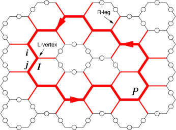
Figure 13: A closed string operator $W(P)$ for the two models (39),(40). The path $P$ is drawn with a thick line, while the legs are drawn with thin lines. The action of the string operators (41),(49) on the legs is different for legs that branch to the right of $P$, “R-legs”, and legs that branch to the left of $P$, “L-legs.” Similarly, we distinguish between “R-vertices” and “L-vertices” which are ends of “R-leg” and “L-leg” respectively.

In the second phase ($\Phi_{-}$), we find

$$\begin{array}[]{llll}n_{1,0}=1,&n_{1,1}=0,&\Omega^{0}_{1,000}=1,&\Omega^{1}_{1,001}=1\\ n_{2,0}=0,&n_{2,1}=1,&\Omega^{1}_{2,110}=1,&\Omega^{0}_{2,111}=i\\ n_{3,0}=0,&n_{3,1}=1,&\Omega^{1}_{3,110}=1,&\Omega^{0}_{3,111}=-i\\ n_{4,0}=1,&n_{4,1}=0,&\Omega^{0}_{4,000}=1,&\Omega^{1}_{4,001}=-1\\ \end{array}$$

Once again, the other elements of $\Omega$ vanish. Also, in all cases, $\bar{\Omega}=\Omega^{*}$. The corresponding string operators for a path $P$ are

$$W_{1} =$$ Id

$$W_{2} = \prod_{\text{edges of }P}\sigma^{z}_{\boldsymbol{j}}\prod_{\text{R-legs}}i^{\frac{1-\sigma^{x}_{\boldsymbol{j}}}{2}}\prod_{\text{L-vertices}}(-1)^{s_{\boldsymbol{I}}}$$

$$W_{3} = \prod_{\text{edges of }P}\sigma^{z}_{\boldsymbol{j}}\prod_{\text{R-legs}}(-i)^{\frac{1-\sigma^{x}_{\boldsymbol{j}}}{2}}\prod_{\text{L-vertices}}(-1)^{s_{\boldsymbol{I}}}$$

$$W_{4} = \prod_{\text{R-legs}}\sigma^{x}_{\boldsymbol{j}}$$ (49)

where the “L-vertices” $\boldsymbol{I}$ are the vertices of $P$ adjacent to legs that are to the left of $P$. The exponent $s_{\boldsymbol{I}}$ is defined by $s_{\boldsymbol{I}}=\frac{1}{4}(1-\sigma^{x}_{\boldsymbol{i}})(1+\sigma^{x}_{\boldsymbol{j}})$, where $\boldsymbol{i}$, $\boldsymbol{j}$ are the links just before and just after the vertex $\boldsymbol{I}$, along the path $P$. (See Fig. 13).

We find the twists and S-matrix are

$$\begin{array}[]{llll}e^{i\theta_{1}}=1,&e^{i\theta_{2}}=i,&e^{i\theta_{3}}=-i,&e^{i\theta_{4}}=1\end{array}$$ (51)

$$S=\frac{1}{2}\left(\begin{array}[]{cccc}1&1&1&1\\ 1&-1&1&-1\\ 1&1&-1&-1\\ 1&-1&-1&1\\ \end{array}\right)$$ (56)

We see that $W_{1}$ creates trivial quasiparticles, $W_{2}$, $W_{3}$ create semions with opposite chiralities and trivial mutual statistics, and $W_{4}$ creates bosonic bound states of the semions. These results agree with the $U(1)\times U(1)$ Chern-Simons theory

$$L=\frac{1}{4\pi}K_{IJ}a_{I\mu}\partial_{\nu}a_{J\lambda}\epsilon^{\mu\nu\lambda},\ \ \ \ \ \ \ I,J=1,2$$ (57)

with $K$-matrix

$$K=\begin{pmatrix}2&0\\ 0&-2\end{pmatrix}$$ (58)

Thus the above $U(1)\times U(1)$ Chern-Simons theory is the low energy effective theory of the second exactly soluble model (with $d_{1}=-1$).

Note that the $Z_{2}$ gauge theory from the first exactly soluble model (with $d_{1}=1$) can also be viewed as a $U(1)\times U(1)$ Chern-Simons theory with $K$-matrix Hansson et al. (2004)

$$K=\begin{pmatrix}0&2\\ 2&0\end{pmatrix}$$ (59)

VI.2 $N=1$ string-net model

The next simplest string-net model also contains only one oriented string type - but with branching. Simple as it is, we will see that this model contains non-Abelian anyons and is theoretically capable of universal fault tolerant quantum computation Freedman et al. (2002). Formally, the model is defined by

1. Number of string types: $N=1$

2. Branching rules: $\{\{1,1,1\}\}$

3. String orientations: $1^{*}=1$.

The string-nets are unoriented trivalent graphs. To find the topological phases that can emerge from these objects, we solve the self-consistency relations (8). We find two sets of self-consistent rules:

$$\Phi\begin{pmatrix}\includegraphics[height=16.62178pt]{Xl.eps}\end{pmatrix}= \gamma_{\pm}\cdot\Phi\begin{pmatrix}\includegraphics[height=16.62178pt]{X0.eps}\end{pmatrix}$$

$$\Phi\begin{pmatrix}\includegraphics[height=16.62178pt]{XijklX.eps}\end{pmatrix}= \gamma_{\pm}^{-1}\cdot\Phi\begin{pmatrix}\includegraphics[height=16.62178pt]{XijX.eps}\end{pmatrix}$$

$$+ \gamma_{\pm}^{-1/2}\cdot\Phi\begin{pmatrix}\includegraphics[height=16.62178pt]{XijklnUX.eps}\end{pmatrix}$$

$$\Phi\begin{pmatrix}\includegraphics[height=16.62178pt]{XijklmUX.eps}\end{pmatrix}= \gamma_{\pm}^{-1/2}\cdot\Phi\begin{pmatrix}\includegraphics[height=16.62178pt]{XijklX.eps}\end{pmatrix}$$

$$- \gamma_{\pm}^{-1}\cdot\Phi\begin{pmatrix}\includegraphics[height=16.62178pt]{XijklnUX.eps}\end{pmatrix}$$ (60)

where $\gamma_{\pm}=\frac{1\pm\sqrt{5}}{2}$. (Once again, we have omitted those rules that can be derived from topological invariance). Unlike the previous case, there is no closed form expression for the wave function amplitude.

Note that the second solution, $d_{1}=\frac{1-\sqrt{5}}{2}$ does not satisfy the unitarity condition (14). Thus, only the first solution corresponds to a physical topological phase. As we will see, this phase is described by an $SO_{3}(3)\times SO_{3}(3)$ Chern-Simons theory.

As before, the exactly soluble realization of this phase (10) is a spin-1/2 model with spins on the links of the honeycomb lattice. We regard a link with $\sigma^{x}=-1$ as being occupied by a type-$1$ string, and a link with $\sigma^{x}=1$ as being unoccupied (or equivalently occupied by a type-$0$ string). However, in this case we will not explicitly rewrite (10) in terms of Pauli matrices, since the resulting expression is quite complicated.

We now find the quasiparticles. These correspond to irreducible solutions of (IV.3). For this model, there are $4$ such solutions, corresponding to $4$ quasiparticles:

$$1:\ \ n_{1,0}=1,\ n_{1,1}=0,\ \Omega^{0}_{1,000}=1,\ \Omega^{1}_{1,001}=1$$

$$2:\ \ n_{2,0}=0,\ n_{2,1}=1,\ \Omega^{1}_{2,110}=1,$$ (61)

$$\ \ \ \Omega^{0}_{2,111}=-\gamma_{+}^{-1}e^{\pi i/5},\ \Omega^{1}_{2,111}=\gamma_{+}^{-1/2}e^{3\pi i/5}$$

$$3:\ \ n_{3,0}=0,\ n_{3,1}=1,\ \Omega^{1}_{3,110}=1,$$

$$\ \ \ \Omega^{0}_{3,111}=-\gamma_{+}^{-1}e^{-\pi i/5},\ \Omega^{1}_{3,111}=\gamma_{+}^{-1/2}e^{-3\pi i/5}$$

$$4:\ \ n_{4,0}=1,\ n_{4,1}=1,\ \Omega^{0}_{4,000}=1,\ \Omega^{1}_{4,110}=1,$$

$$\ \ \ \Omega^{1}_{4,001}=-\gamma_{+}^{-2},\ \Omega^{0}_{4,111}=\gamma_{+}^{-1},\ \Omega^{1}_{4,111}=\gamma_{+}^{-5/2},$$

$$\ \ \ \Omega^{1}_{4,101}=(\Omega^{1}_{4,011})^{*}=\gamma_{+}^{-11/4}(2-e^{3\pi i/5}+\gamma_{+}e^{-3\pi i/5}).$$

In all cases, $\bar{\Omega}=\Omega^{*}$.

We can calculate the twists and the S-matrix. We find:

$$\begin{array}[]{llll}e^{i\theta_{1}}=1,&e^{i\theta_{2}}=e^{-4\pi i/5},&e^{i\theta_{3}}=e^{4\pi i/5},&e^{i\theta_{4}}=1\end{array}$$ (63)

$$S=\frac{1}{1+\gamma^{2}}\left(\begin{array}[]{cccc}1&\gamma&\gamma&\gamma^{2}\\ \gamma&-1&\gamma^{2}&-\gamma\\ \gamma&\gamma^{2}&-1&-\gamma\\ \gamma^{2}&-\gamma&-\gamma&1\\ \end{array}\right)$$ (68)

We conclude that $W_{1}$ creates trivial quasiparticles, $W_{2}$, $W_{3}$ create (non-Abelian) anyons with opposite chiralities, and $W_{4}$ creates bosonic bound states of the anyons. These results agree with $SO_{3}(3)\times SO_{3}(3)$ Chern-Simons theory, the so-called doubled “Yang-Lee” theory.

Researchers in the field of quantum computing have shown that the Yang-Lee theory can function as a universal quantum computer - via manipulation of non-Abelian anyons. Freedman et al. (2002) Therefore, the spin-1/2 Hamiltonian (10) associated with (VI.2) is a theoretical realization of a universal quantum computer. While this Hamiltonian may be too complicated to be realized experimentally, the string-net picture suggests that this problem can be overcome. Indeed, the string-net picture suggests that generic spin Hamiltonians with a trivalent graph structure will exhibit a Yang-Lee phase. Thus, much simpler spin-1/2 Hamiltonians may be capable of universal fault tolerant quantum computation.

VI.3 $N=2$ string-net models

In this section, we discuss two $N=2$ string-net models. The first model contains one oriented string and its dual. In the notation from section III, it is given by

1. Number of string types: $N=2$

2. Branching rules: $\{\{1,1,1\},\{2,2,2\}\}$

3. String orientations: $1^{*}=2$, $2^{*}=1$.

The string-nets are therefore oriented trivalent graphs with $Z_{3}$ branching rules. The string-net condensed phases correspond to solutions of (8). Solving these equations, we find two sets of self-consistent local rules:

$$\Phi\begin{pmatrix}\includegraphics[height=16.62178pt]{Xl0.eps}\end{pmatrix}= \pm\Phi\begin{pmatrix}\includegraphics[height=16.62178pt]{X0.eps}\end{pmatrix}$$

$$\Phi\begin{pmatrix}\includegraphics[height=16.62178pt]{XijklXO.eps}\end{pmatrix}= \pm\Phi\begin{pmatrix}\includegraphics[height=16.62178pt]{XijXO.eps}\end{pmatrix}$$

$$\Phi\begin{pmatrix}\includegraphics[height=16.62178pt]{XijklXPO.eps}\end{pmatrix}= \sqrt{\pm 1}\cdot\Phi\begin{pmatrix}\includegraphics[height=16.62178pt]{XijklnUXO.eps}\end{pmatrix}$$ (69)

The corresponding fixed-point wave functions $\Phi_{\pm}$ are given by

$$\Phi_{\pm}(X)=(\sqrt{\pm 1})^{2X_{c}-X_{v}/2}$$ (70)

where $X_{c}$, $X_{v}$, are the number of connected components, and vertices, respectively in the string-net configuration $X$. As before, we can construct an exactly soluble Hamiltonians, find the quasiparticles for the two theories and compute the twists and S-matrices. We find that the first theory $\Phi_{+}$ is described by a $Z_{3}$ gauge theory, while the second theory $\Phi_{-}$ is described by a $U(1)\times U(1)$ Chern-Simons theory with $K$-matrix

$$K=\begin{pmatrix}3&0\\ 0&-3\end{pmatrix}$$

Both theories have $3^{2}=9$ elementary quasiparticles. In the case of $Z_{3}$, these quasiparticles are electric charge/magnetic flux bound states formed from the $3$ types of electric charges and $3$ types of magnetic fluxes. In the case of the Chern-Simons theory, the quasiparticles are bound states of the two fundamental anyons with statistical angles $\pm\pi/3$.

The final example we will discuss contains two unoriented strings. Formally it is given by

1. Number of string types: $N=2$

2. Branching rules: $\{\{1,2,2\},\{2,2,2\}\}$

3. String orientations: $1^{*}=1$, $2^{*}=2$.

The string-nets are unoriented trivalent graphs, with edges labeled with $1$ or $2$. We find that there is only one set of self-consistent local rules:

$$\Phi\begin{pmatrix}\includegraphics[height=16.62178pt]{Xil0.eps}\end{pmatrix}= d_{i}\cdot\Phi\begin{pmatrix}\includegraphics[height=16.62178pt]{X0.eps}\end{pmatrix}$$

$$\Phi\begin{pmatrix}\includegraphics[height=16.62178pt]{X1111m.eps}\end{pmatrix}= \Phi\begin{pmatrix}\includegraphics[height=16.62178pt]{X1111n.eps}\end{pmatrix}$$

$$\Phi\begin{pmatrix}\includegraphics[height=16.62178pt]{X1221m.eps}\end{pmatrix}= \Phi\begin{pmatrix}\includegraphics[height=16.62178pt]{X1221n.eps}\end{pmatrix}$$

$$\Phi\begin{pmatrix}\includegraphics[height=16.62178pt]{X1212m.eps}\end{pmatrix}= \Phi\begin{pmatrix}\includegraphics[height=16.62178pt]{X1212n.eps}\end{pmatrix}$$

$$\Phi\begin{pmatrix}\includegraphics[height=16.62178pt]{X1222m.eps}\end{pmatrix}= -\Phi\begin{pmatrix}\includegraphics[height=16.62178pt]{X1222n.eps}\end{pmatrix}$$

$$\Phi\begin{pmatrix}\includegraphics[height=16.62178pt]{XmX.eps}\end{pmatrix}= \sum_{n=0}^{2}F^{22m}_{22n}\cdot\Phi\begin{pmatrix}\includegraphics[height=16.62178pt]{XnX.eps}\end{pmatrix}$$ (71)

where $d_{0}=d_{1}=1$, $d_{2}=2$, and $F^{22m}_{22n}$ is the matrix

$$F^{22m}_{22n}=\begin{pmatrix}\frac{1}{2}&\frac{1}{2}&\frac{1}{\sqrt{2}}\\ \frac{1}{2}&\frac{1}{2}&-\frac{1}{\sqrt{2}}\\ \frac{1}{\sqrt{2}}&-\frac{1}{\sqrt{2}}&0\end{pmatrix}$$

If we construct the Hamiltonian (10), we find that it is equivalent to the standard exactly lattice gauge theory Hamiltonian Kitaev (2003) with gauge group $S_{3}$ - the permutation group on $3$ objects. One can show that this theory contains $8$ elementary quasiparticles (corresponding to the $8$ irreducible representations of the quantum double $D(S_{3})$). These quasiparticles are combinations of the $3$ electric charges and $3$ magnetic fluxes.

VII Conclusion

In this paper, we have shown that quantum systems of extended objects naturally give rise to topological phases. These phases occur when the extended objects (e.g. string-nets) become highly fluctuating and condense. This physical picture provides a natural mechanism for the emergence of parity invariant topological phases. Microscopic degrees of freedoms (such as spins or dimers) can organize into effective extended objects which can then condense. We hope that this physical picture may help direct the search for topological phases in real condensed matter systems. It would be interesting to develop an analogous picture for chiral topological phases.

We have also found the fundamental mathematical framework for topological phases. We have shown that each $(2+1)$ dimensional doubled topological phase is associated with a $6$ index object $F^{ijm}_{kln}$ and a set of real numbers $d_{i}$ satisfying the algebraic relations (8). All the universal properties of the topological phase are contained in these mathematical objects (known as tensor categories). In particular, the tensor category directly determines the quasiparticle statistics of the associated topological phase (28, 30). This mathematical framework may also have applications to phase transitions and critical phenomena. Tensor categories may characterize transitions between topological phases just as symmetry groups characterize transitions between ordered phases.

We have constructed exactly soluble $(2+1)D$ lattice spin Hamiltonians (10) realizing each of these doubled topological phases. These models unify $(2+1)D$ lattice gauge theory and doubled Chern-Simons theory. One particular Hamiltonian - a realization of the doubled Yang-Lee theory - is a spin 1/2 model capable of fault tolerant quantum computation.

In higher dimensions, string-nets can also give rise to topological phases. However, the physical and mathematical structure of these phases is more restricted. On a mathematical level, each higher dimensional string-net condensate is associated with a special kind of tensor category - a symmetric tensor category (IV.3), (32). More physically, we have shown that higher dimensional string-net condensation naturally gives rise to both gauge interactions and Fermi statistics. Viewed from this perspective, string-net condensation provides a mechanism for unifying gauge interactions and Fermi statistics. It may have applications to high energy physics Wen (2003a).

From a more general point of view, all of the phases described by Landau’s symmetry breaking theory can be understood in terms of particle condensation. These phases are classified using group theory and lead to emergent gapless scalar bosons Nambu (1960); Goldstone (1961), such as phonons, spin waves, etc . In this paper, we have shown that there is a much richer class of phase - arising from the condensation of extended objects. These phases are classified using tensor category theory and lead to emergence of Fermi statistics and gauge excitations. Clearly, there is whole new world beyond the paradigm of symmetry breaking and long range order. It is a virgin land waiting to be explored.

We would like to thank Pavel Etingof and Michael Freedman for useful discussions of the mathematical aspects of topological field theory. This research is supported by NSF Grant No. DMR–01–23156 and by NSF-MRSEC Grant No. DMR–02–13282.

Appendix A General string-net models

In this section, we discuss the most general string-net models. These models can describe all doubled topological phases, including all discrete gauge theories and doubled Chern-Simons theories.

In these models, there is a “spin” degree of freedom at each branch point or node of a string-net, in addition to the usual string-net degrees of freedom. The dimension of this “spin” Hilbert space depends on the string types of the $3$ strings incident on the node.

To specify a particular model one needs to provide a $3$ index tensor $\delta_{ijk}$ which gives the dimension of the spin Hilbert space associated with $\{i,j,k\}$ (in addition to the usual information). The string-net models discussed above correspond to the special case where $\delta_{ijk}=0,1$ for all $i,j,k$. In the case of gauge theory, $\delta_{ijk}$ is the number of copies of the trivial representation that appear in the tensor product $i\otimes j\otimes k$. Thus we need the more general string-net picture to describe gauge theories where the trivial representation appears multiple times in $i\otimes j\otimes k$.

The Hilbert space of the string-net model is defined in the natural way: the states in the string-net Hilbert space are linear superpositions of different spatial configurations of string-nets with different spin states at the nodes.

One can analyze string-net condensed phases as before. The universal properties of each phase are captured by a fixed-point ground state wave function $\Phi$. The wave function $\Phi$ is specified by the local rules (4), (5) and simple modifications of (6), (7):

$$\Phi\begin{pmatrix}\includegraphics[height=21.68121pt]{XikljsO.eps}\end{pmatrix}= \delta_{ij}\delta_{\sigma\tau}\Phi\begin{pmatrix}\includegraphics[height=21.68121pt]{XiklisO.eps}\end{pmatrix}$$

$$\Phi\begin{pmatrix}\includegraphics[height=26.01724pt]{XijklmsXO.eps}\end{pmatrix}= \sum_{n\mu\nu}(F^{ijm}_{kln})^{\sigma\tau}_{\mu\nu}\Phi\begin{pmatrix}\includegraphics[height=21.68121pt]{XijklnsXO.eps}\end{pmatrix}$$

The complex numerical constant $F^{ijm}_{kln}$ is now a complex tensor $(F^{ijm}_{kln})^{\sigma\tau}_{\mu\nu}$ of dimension $\delta_{ijm}\times\delta_{klm^{*}}\times\delta_{inl}\times\delta_{jkn^{*}}$.

One can proceed as before, with self-consistency conditions, fixed-point Hamiltonians, string operators, and the generalization to $(3+1)$ dimensions. The exactly soluble models are similar to (10). The main difference is the existence of an additional spin degree of freedom at each site of the honeycomb lattice. These spins account for the degrees of freedom at the nodes of the string-nets.

Appendix B Self-consistency conditions

In this section, we derive the self-consistency conditions (8). We begin with the last relation, the so-called “pentagon identity”, since it is the most fundamental. To derive this condition, we use the fusion rule (7) to relate the amplitude $\Phi\left(\begin{matrix}\includegraphics[height=28.90755pt]{pen1O.eps}\end{matrix}\right)$ to the amplitude $\Phi\left(\begin{matrix}\includegraphics[height=28.90755pt]{pen3O.eps}\end{matrix}\right)$ in two distinct ways (see Fig. 14). On the one hand, we can apply the fusion rule (7) twice to obtain the relation

$$\Phi\left(\begin{matrix}\includegraphics[height=28.90755pt]{pen1O.eps}\end{matrix}\right)= \sum_{r}F^{jip}_{q^{*}kr^{*}}\Phi\left(\begin{matrix}\includegraphics[height=28.90755pt]{pen2O.eps}\end{matrix}\right)$$

$$= \sum_{r,s}F^{jip}_{q^{*}kr^{*}}F^{riq^{*}}_{mls^{*}}\Phi\left(\begin{matrix}\includegraphics[height=28.90755pt]{pen3O.eps}\end{matrix}\right)$$

(Here, we neglected to draw a shaded region surrounding the whole diagram. Just as in the local rules (4-7) the ends of the strings $i,j,k,l,m$ are connected to some arbitrary string-net configuration). But we can also apply the fusion rule (7) three times to obtain a different relation:

$$\Phi\left(\begin{matrix}\includegraphics[height=28.90755pt]{pen1O.eps}\end{matrix}\right)= \sum_{n}F^{mlq}_{kp^{*}n}\Phi\left(\begin{matrix}\includegraphics[height=28.90755pt]{pen4O.eps}\end{matrix}\right)$$

$$= \sum_{n,s}F^{mlq}_{kp^{*}n}F^{jip}_{mns^{*}}\Phi\left(\begin{matrix}\includegraphics[height=28.90755pt]{pen5O.eps}\end{matrix}\right)$$

$$= \sum_{n,r,s}F^{mlq}_{kp^{*}n}F^{jip}_{mns^{*}}F^{js^{*}n}_{lkr^{*}}\Phi\left(\begin{matrix}\includegraphics[height=28.90755pt]{pen3O.eps}\end{matrix}\right)$$

If the rules are self-consistent, then these two relations must agree with each other. Thus, the two coefficients of $\Phi\left(\begin{matrix}\includegraphics[height=28.90755pt]{pen3O.eps}\end{matrix}\right)$ must be the same. This equality implies the pentagon identity (8).

Figure 14: The fusion rule (7) can be used to relate the amplitude of (a) to the amplitude of (c) in two different ways. On the one hand, we can apply the fusion rule (7) twice - along the links denoted by solid arrows - to relate (a) $\to$ (b) $\to$ (c). But we can also apply (7) three times - along the links denoted by dashed arrows - to relate (a) $\to$ (d) $\to$ (e) $\to$ (c). Self-consistency requires that the two sequences of the operation lead to the same linear relations between the amplitudes of (a) and (c).

The first two relations in (8) are less fundamental. In fact, the first relation is not required by self-consistency at all; it is simply a useful convention. To see this, consider the following rescaling transformation on wave functions $\Phi\to\tilde{\Phi}$. Given a string-net wave function $\Phi$, we can obtain a new wave function $\tilde{\Phi}$ by multiplying the amplitude $\Phi(X)$ for a string-net configuration $X$ by an arbitrary factor $f(i,j,k)$ for each vertex $\{i,j,k\}$ in $X$. As long as $f(i,j,k)$ is symmetric in $i,j,k$ and $f(0,i,i^{*})=1$, this operation preserves the topological invariance of $\Phi$. The rescaled wave function $\tilde{\Phi}$ satisfies the same set of local rules with rescaled $F^{ijm}_{kln}$:

$$F^{ijm}_{kln}\to\tilde{F}^{ijm}_{kln}=F^{ijm}_{kln}\frac{f(i,j,m)f(k,l,m^{*})}{f(n,l,i)f(j,k,n^{*})}$$ (72)

Since $\Phi$ and $\tilde{\Phi}$ describe the same quantum phase, we regard $F$ and $\tilde{F}$ as equivalent local rules. Thus the first relation in (8) is simply a normalization convention for $F$ or $\Phi$ (except when $i,j$ or $k$ vanishes; these cases require an argument similar to the derivation of the pentagon identity).

The second relation in (8) has more content. This relation can be derived by computing the amplitude for a tetrahedral string-net configuration. We have:

$$\Phi\begin{pmatrix}\includegraphics[width=28.90755pt]{FG0.eps}\end{pmatrix}=F^{ijm}_{kln}\Phi\begin{pmatrix}\includegraphics[height=31.07556pt]{FG1.eps}\end{pmatrix}$$

$$= F^{ijm}_{kln}F^{nk^{*}j^{*}}_{kn^{*}0}d_{k}\Phi\begin{pmatrix}\includegraphics[height=28.90755pt]{FG2.eps}\end{pmatrix}$$

$$= F^{ijm}_{kln}F^{nk^{*}j^{*}}_{kn^{*}0}F^{n^{*}i^{*}l^{*}}_{in0}d_{k}d_{i}d_{n}\Phi(\emptyset)$$ (73)

$$= F^{ijm}_{kln}v_{i}v_{j}v_{k}v_{l}\Phi(\emptyset)$$ (74)

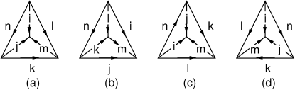
Figure 15: Four string-net configurations related by tetrahedral symmetry. In diagram (a), we show the tetrahedron corresponding to $G^{ijm}_{kln}$. In diagrams (b), (c),(d), we show the tetrahedrons $G^{lkm^{*}}_{jin}$, $G^{jim}_{lkn^{*}}$, $G^{imj}_{k^{*}nl}$, obtained by reflecting (a) in $3$ different planes: the plane joining $n$ to the center of $m$, the plane joining $m$ to the center of $n$, and the plane joining $i$ to the center of $k$. The four tetrahedrons correspond to the four terms in the second relation of (8).

We define the above combination in the front of $\Phi(\emptyset)$ as:

$$G^{ijm}_{kln}\equiv F^{ijm}_{kln}v_{i}v_{j}v_{k}v_{l}$$ (75)

Imagine that the above string-net configuration lies on a sphere. In that case, topological invariance (together with parity invariance) requires that $G^{ijm}_{kln}$ be invariant under all $24$ symmetries of a regular tetrahedron. The second relation in (8) is simply a statement of this tetrahedral symmetry requirement - written in terms of $F^{ijm}_{kln}$. (See Fig. 15).

In this section, we have shown that the relations (8) are necessary for self-consistency. It turns out that these relations are also sufficient. One way of proving this is to use the lattice model (10). A straightforward algebraic calculation shows that the ground state of 10 obeys the local rules (4-7), as long as (8) is satisfied. This establishes that the local rules are self-consistent.

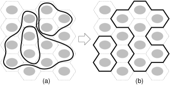
Figure 16: The fattened honeycomb lattice. The strings are forbidden in the shaded region. A string state in the fattened honeycomb lattice (a) can be viewed as a superposition of string states on the links (b).

Appendix C Graphical representation of the Hamiltonian

In this section, we provide an alternative, graphical, representation of the lattice model (10). This graphical representation provides a simple visual technique for understanding properties (a)-(c) of the Hamiltonian (10).

We begin with the $2D$ honeycomb lattice. Imagine we fatten the links of the lattice into stripes of finite width (see Fig. 16). Then, any string-net state in the fattened honeycomb lattice (Fig. 16a) can be viewed as a superposition of string-net states in the original, unfattened lattice (Fig. 16b). This mapping is obtained via the local rules (4-7). Using these rules, we can relate the amplitude $\Phi(X)$ for a string-net in the fattened lattice to a linear combination of string-net amplitudes in the original lattice: $\Phi(X)=\sum a_{i}\Phi(X_{i})$. This provides a natural linear relation between the states in the fattened lattice and those in the unfattened lattice: $|X\rangle=\sum a_{i}|X_{i}\rangle$. This linear relation is independent of the particular way in which the local rules (4-7) are applied, as long as the rules are self-consistent.

In this way, the fattened honeycomb lattice provides an alternative notation for representing the states in the Hilbert space of (10). This notation is useful because the magnetic energy operators $B^{s}_{\boldsymbol{p}}$ are simple in this representation. Indeed, the action of the operator $B^{s}_{\boldsymbol{p}}$ on the string-net state $\Big{|}\begin{matrix}\includegraphics[height=43.36243pt]{BsL0O.eps}\end{matrix}\Big{\rangle}$ is equivalent to simply adding a loop of type-$s$ string:

$$B^{s}_{\boldsymbol{p}}\Big{|}\begin{matrix}\includegraphics[height=57.81621pt]{BsL0O.eps}\end{matrix}\Big{\rangle}=\Big{|}\begin{matrix}\includegraphics[height=57.81621pt]{BsL1O.eps}\end{matrix}\Big{\rangle}$$

As we described above, we can use the local rules (4-7) to rewrite $\Big{|}\begin{matrix}\includegraphics[height=43.36243pt]{BsL1O.eps}\end{matrix}\Big{\rangle}$ as a linear combination of the physical string-net states with strings only on the links, that is to reduce Fig. 17a to Fig. 17b. This allows us to obtain the matrix elements of $B^{s}_{\boldsymbol{p}}$.

The following is a particular way to implement the above procedure:

$$B^{s}_{\boldsymbol{p}}\Big{|}\begin{matrix}\includegraphics[height=57.81621pt]{BsL0O.eps}\end{matrix}\Big{\rangle}=\Big{|}\begin{matrix}\includegraphics[height=57.81621pt]{BsL10O.eps}\end{matrix}\Big{\rangle}=\sum_{g^{\prime}h^{\prime}i^{\prime}j^{\prime}k^{\prime}l^{\prime}}F^{gg^{*}0}_{s^{*}sg^{\prime*}}F^{hh^{*}0}_{s^{*}sh^{\prime*}}F^{ii^{*}0}_{s^{*}si^{\prime*}}F^{jj^{*}0}_{s^{*}sj^{\prime*}}F^{kk^{*}0}_{s^{*}sk^{\prime*}}F^{ll^{*}0}_{s^{*}sl^{\prime*}}\Big{|}\begin{matrix}\includegraphics[height=57.81621pt]{BsL11O.eps}\end{matrix}\Big{\rangle}$$

$$= \sum_{g^{\prime}h^{\prime}i^{\prime}j^{\prime}k^{\prime}l^{\prime}}F^{gg^{*}0}_{s^{*}sg^{\prime*}}F^{hh^{*}0}_{s^{*}sh^{\prime*}}F^{ii^{*}0}_{s^{*}si^{\prime*}}F^{jj^{*}0}_{s^{*}sj^{\prime*}}F^{kk^{*}0}_{s^{*}sk^{\prime*}}F^{ll^{*}0}_{s^{*}sl^{\prime*}}F^{bg^{*}h}_{s^{*}h^{\prime}g^{\prime*}}F^{ch^{*}i}_{s^{*}i^{\prime}h^{\prime*}}F^{di^{*}j}_{s^{*}j^{\prime}i^{\prime*}}F^{ej^{*}k}_{s^{*}k^{\prime}j^{\prime*}}F^{fk^{*}l}_{s^{*}l^{\prime}k^{\prime*}}F^{al^{*}g}_{s^{*}g^{\prime}l^{\prime*}}\Big{|}\begin{matrix}\includegraphics[height=57.81621pt]{BsL12O.eps}\end{matrix}\Big{\rangle}$$

$$= \sum_{g^{\prime}h^{\prime}i^{\prime}j^{\prime}k^{\prime}l^{\prime}}F^{bg^{*}h}_{s^{*}h^{\prime}g^{\prime*}}F^{ch^{*}i}_{s^{*}i^{\prime}h^{\prime*}}F^{di^{*}j}_{s^{*}j^{\prime}i^{\prime*}}F^{ej^{*}k}_{s^{*}k^{\prime}j^{\prime*}}F^{fk^{*}l}_{s^{*}l^{\prime}k^{\prime*}}F^{al^{*}g}_{s^{*}g^{\prime}l^{\prime*}}\Big{|}\begin{matrix}\includegraphics[height=57.81621pt]{BsL6O.eps}\end{matrix}\Big{\rangle}$$ (76)

Notice that (C) is exactly (IV.2). Thus, the graphical representation of $B^{s}_{\boldsymbol{p}}$ agrees with the original algebraic definition.

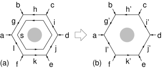
Figure 17: The action of $B^{s}_{\boldsymbol{p}}$ is equivalent to adding a loop of type-$s$ string. The resulting string-net state (a) is actually a linear combination of the string-net states (b). The coefficients in this linear relation can be obtained by using the local rules (4-7) to reduce (a) to (b).

Using the graphical representation of $B^{s}_{\boldsymbol{p}}$ we can easily show that $B^{s_{1}}_{\boldsymbol{p_{1}}}$ and $B^{s_{2}}_{\boldsymbol{p_{2}}}$ commute. The derivation is much simpler then the more straightforward algebraic calculation. First note that these operators will commute if $\boldsymbol{p_{1}}$, $\boldsymbol{p_{2}}$ are well-separated. Thus, we only have to consider the case where $\boldsymbol{p_{1}}$ and $\boldsymbol{p_{2}}$ are adjacent, or the case where $\boldsymbol{p_{1}}$, $\boldsymbol{p_{2}}$ coincide. We begin with the nearest neighbor case. The action of $B^{s_{1}}_{\boldsymbol{p_{1}}}B^{s_{2}}_{\boldsymbol{p_{2}}}$ on the string-net state Fig. 18a can be represented as Fig. 18b. Fig. 18b can then be related to a linear combination of the string-net states shown in Fig. 18c. The coefficients in this relation are the matrix elements of $B^{s_{1}}_{\boldsymbol{p}_{1}}B^{s_{2}}_{\boldsymbol{p}_{2}}$. But by the same argument, the action of $B^{s_{2}}_{\boldsymbol{p}_{2}}B^{s_{1}}_{\boldsymbol{p}_{1}}$ can also be represented by Fig. 18b. We conclude that $B^{s_{2}}_{\boldsymbol{p}_{2}}B^{s_{1}}_{\boldsymbol{p}_{1}}$, $B^{s_{1}}_{\boldsymbol{p}_{1}}B^{s_{2}}_{\boldsymbol{p}_{2}}$ have the same matrix elements. Thus, the two operators commute in this case.

On the other hand, when $\boldsymbol{p}_{1}=\boldsymbol{p}_{2}$, we have

$$B^{s_{2}}_{\boldsymbol{p}}B^{s_{1}}_{\boldsymbol{p}}\Big{|}\begin{matrix}\includegraphics[height=43.36243pt]{BBc0.eps}\end{matrix}\Big{\rangle}=\Big{|}\begin{matrix}\includegraphics[height=43.36243pt]{BBc1O.eps}\end{matrix}\Big{\rangle}$$

$$= \sum_{k}F^{s_{1}s_{1}^{*}0}_{s_{2}^{*}s_{2}k^{*}}\Big{|}\begin{matrix}\includegraphics[height=43.36243pt]{BBc2O.eps}\end{matrix}\Big{\rangle}$$

$$= \sum_{k}F^{s_{1}s_{1}^{*}0}_{s_{2}^{*}s_{2}k^{*}}F^{k^{*}s_{2}s_{1}}_{s_{2}^{*}k0}d_{s_{2}^{*}}\Big{|}\begin{matrix}\includegraphics[height=43.36243pt]{BBc3O.eps}\end{matrix}\Big{\rangle}$$

$$= \sum_{k}\delta_{k^{*}s_{2}s_{1}}\Big{|}\begin{matrix}\includegraphics[height=43.36243pt]{BBc3O.eps}\end{matrix}\Big{\rangle}$$ (77)

Thus,

$$B^{s_{2}}_{\boldsymbol{p}}B^{s_{1}}_{\boldsymbol{p}}=\sum_{k}\delta_{k^{*}s_{2}s_{1}}B^{k}_{\boldsymbol{p}}.$$ (78)

Since $\delta_{k^{*}s_{2}s_{1}}$ is symmetric in $s_{2}$, $s_{1}$, we conclude that $B^{s_{1}}_{\boldsymbol{p}}B^{s_{2}}_{\boldsymbol{p}}=B^{s_{2}}_{\boldsymbol{p}}B^{s_{1}}_{\boldsymbol{p}}$, so the operators commute in this case as well. This establishes property (a) of the Hamiltonian (10).

Figure 18: The action of $B^{s_{1}}_{\boldsymbol{p_{1}}}B^{s_{2}}_{\boldsymbol{p_{2}}}$ on the string-net state (a) can be represented by adding two loops of type-$s_{1}$ and type-$s_{2}$ strings as shown in (b). The string-net state (b) is a linear combination of the string-net states (c). The coefficients are obtained by using (4 -7) to reduce (b) to (c).

Equation (78) also sheds light on the spectrum of the $B^{s}_{\boldsymbol{p}}$ operators. Let the simultaneous eigenvalues of $B^{s}_{\boldsymbol{p}}$ (with $\boldsymbol{p}$ fixed) be $\{b^{s}_{q}\}$. Then, by (78) these eigenvalues satisfy

$$\sum_{k}\delta_{k^{*}s_{2}s_{1}}b^{k}_{q}=b^{s_{2}}_{q}b^{s_{1}}_{q}$$

We can view this as an eigenvalue equation for the $(N+1)\times(N+1)$ matrix $M_{s_{2}}$, defined by $M^{i}_{s_{2},j}=\delta_{j^{*}s_{2}i}$. The simultaneous eigenvalues $b^{s_{2}}_{q}$ are simply the simultaneous eigenvalues of the matrices $M_{s_{2}}$. In particular, this means that the index $q$ ranges over a set of size $N+1$.

Each value of $q$ corresponds to a different possible state for the plaquette $\boldsymbol{p}$. The magnetic energies of these $N+1$ different states are given by: $E_{q}=-\sum_{s}a_{s}b^{s}_{q}$. Depending on the parameter choice $a_{s}$, all on the plaquettes $\boldsymbol{p}$ will be in one of these states $q$. In this way, the Hamiltonian (10) can be in $N+1$ different quantum phase. This establishes property (b) of the Hamiltonian (10).

One particular state $q$ is particularly interesting. This state corresponds to the simultaneous eigenvalues $b^{s}=d_{s}$. It is not hard to show that the parameter choice $a_{s}=\frac{d_{s}}{\sum_{k}d_{k}^{2}}$ makes this state energetically favorable. In fact, using (78) one can show that $B_{\boldsymbol{p}}$ is a projector for this parameter choice, and that $B_{\boldsymbol{p}}=1$ for this state.

Furthermore, the ground state wave function for this parameter choice obeys the local rules (4-7). One way to see this is to compare $B_{\boldsymbol{p}}\Big{|}\begin{matrix}\includegraphics[width=32.52127pt]{hop0O.eps}\end{matrix}\Big{\rangle}$ with $B_{\boldsymbol{p}}\Big{|}\begin{matrix}\includegraphics[width=32.52127pt]{hop0aO.eps}\end{matrix}\Big{\rangle}$. For the first state, we find

$$B_{\boldsymbol{p}}\Big{|}\begin{matrix}\includegraphics[width=32.52127pt]{hop0O.eps}\end{matrix}\Big{\rangle}= \sum_{s}a_{s}\Big{|}\begin{matrix}\includegraphics[width=32.52127pt]{hop1O.eps}\end{matrix}\Big{\rangle}$$

$$= \sum_{j,s}\frac{d_{s}}{\sum_{k}d_{k}^{2}}F^{ii^{*}0}_{s^{*}sj^{*}}\Big{|}\begin{matrix}\includegraphics[width=32.52127pt]{hop3O.eps}\end{matrix}\Big{\rangle}$$

$$= \sum_{j,s}\frac{v_{j}v_{s}}{v_{i}\sum_{k}d_{k}^{2}}\Big{|}\begin{matrix}\includegraphics[width=32.52127pt]{hop3O.eps}\end{matrix}\Big{\rangle}$$

For the second state, we find the same result:

$$B_{\boldsymbol{p}}\Big{|}\begin{matrix}\includegraphics[width=32.52127pt]{hop0aO.eps}\end{matrix}\Big{\rangle}=\sum_{j,s}\frac{v_{j}v_{s}}{v_{i}\sum_{k}d_{k}^{2}}\Big{|}\begin{matrix}\includegraphics[width=32.52127pt]{hop3aO.eps}\end{matrix}\Big{\rangle}$$

It follows that

$$0 =\Big{\langle}\begin{matrix}\includegraphics[width=32.52127pt]{hop0O.eps}\end{matrix}\Big{|}B_{\boldsymbol{p}}\Big{|}\Phi\Big{\rangle}-\Big{\langle}\begin{matrix}\includegraphics[width=32.52127pt]{hop0aO.eps}\end{matrix}\Big{|}B_{\boldsymbol{p}}\Big{|}\Phi\Big{\rangle}$$

$$=\Big{\langle}\begin{matrix}\includegraphics[width=32.52127pt]{hop0O.eps}\end{matrix}\Big{|}\Phi\Big{\rangle}-\Big{\langle}\begin{matrix}\includegraphics[width=32.52127pt]{hop0aO.eps}\end{matrix}\Big{|}\Phi\Big{\rangle}$$

so

$$\Phi\begin{pmatrix}\includegraphics[width=32.52127pt]{hop0O.eps}\end{pmatrix}=\Phi\begin{pmatrix}\includegraphics[width=32.52127pt]{hop0aO.eps}\end{pmatrix}$$

This result means that the strings can be moved through the forbidden regions at the center of the hexagons. Thus, the local rules which were originally restricted to the fattened honeycomb lattice can be extended throughout the entire $2D$ plane. The wave function $\Phi$ obeys these continuum local rules and has a smooth continuum limit. We call such a state smooth topological state. This establishes property (c) of the Hamiltonian (10).

The wave functions of some smooth topological states are positive definite. So those wave functions can be viewed as the statistical weights of certain statistical models in the same spatial dimensions. What is interesting is that those statistical models are local models with short-ranged interactions Witten (1989b, 1990); Ardonne et al. (2004).

Appendix D Graphical representation of the string operators

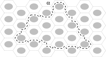
Figure 19: The action of the string operator $W_{\alpha}(P)$ is equivalent to adding a type-$\alpha$ string along the path $P$. The resulting string-net state can be reduced to a linear combination of states on the honeycomb lattice, using the local rules (4-7), (79).

In this section, we describe a graphical representation of the long string operators $W_{\alpha}(P)$. Just as in the previous section, this representation involves the fattened honeycomb lattice. The action of the string operator $W_{\alpha}(P)$ on a general string state $X$, is simply to create a string labeled $\alpha$ along the path $P$. The resulting string-net state can then be reduced to a linear combination of string-net states on the unfattened lattice. The coefficients in this linear combination are the matrix elements of $W_{\alpha}(P)$.

However, none of the rules (4-7) involve strings labeled $\alpha$, nor do they allow for crossings. Thus, the reduction to string-net states on the unfattened lattice requires new local rules. These new local rules are defined by the $4$ index objects $\Omega^{j}_{\alpha,sti}$, $\bar{\Omega}^{j}_{\alpha,sti}$, and the integers $n_{\alpha,i}$:

$$\Big{|}\begin{matrix}\includegraphics[height=21.68121pt]{Xal0.eps}\end{matrix}\Big{\rangle} = \sum_{i}n_{\alpha,i}\Big{|}\begin{matrix}\includegraphics[height=21.68121pt]{Xil0.eps}\end{matrix}\Big{\rangle}$$

$$\Big{|}\begin{matrix}\includegraphics[height=21.68121pt]{Brd1O.eps}\end{matrix}\Big{\rangle} = \sum_{jst}(\Omega^{j}_{\alpha,sti})_{\sigma\tau}\Big{|}\begin{matrix}\includegraphics[height=21.68121pt]{Brd2O.eps}\end{matrix}\Big{\rangle}$$

$$\Big{|}\begin{matrix}\includegraphics[height=21.68121pt]{Brd1aO.eps}\end{matrix}\Big{\rangle} = \sum_{jst}(\bar{\Omega}^{j}_{\alpha,sti})_{\sigma\tau}\Big{|}\begin{matrix}\includegraphics[height=21.68121pt]{Brd2aO.eps}\end{matrix}\Big{\rangle}$$ (79)

Here, $\sigma,\tau$ are the two indices of the matrix $\Omega^{ij}_{st}$. (Until now, we’ve neglected to write out these indices explicitly).

After applying these rules, we then need to join together the resulting string-nets. The “joining rule” for two string types $s_{1}$, $s_{2}$ is as follows. If $s_{1}\neq s_{2}$, we don’t join the two strings: we simply throw away the diagram. If $s_{1}=s_{2}$, then we join the two strings and contract the two corresponding indices $\sigma_{1}$, $\sigma_{2}$. That is, we multiply the two $\Omega$ matrices together in the usual way. Using the same approach as (C), one can show that the graphical definition of $W_{\alpha}(P)$ agrees with the algebraic definition (19).

In the previous section, we used the graphical representation of $B^{s}_{\boldsymbol{p}}$ to show that these operators commute. The string operators $W_{\alpha}(P)$ can be analyzed in the same way. With a simple graphical argument one can show that the string operators $W_{\alpha}(P)$ commute with the magnetic operators $B^{s}_{\boldsymbol{p}}$ provided that (4-7),(79) satisfy the conditions

$$\Big{|}\begin{matrix}\includegraphics[width=32.52127pt]{Brd3O.eps}\end{matrix}\Big{\rangle} = \Big{|}\begin{matrix}\includegraphics[width=32.52127pt]{Brd4O.eps}\end{matrix}\Big{\rangle}$$ (80)

$$\Big{|}\begin{matrix}\includegraphics[height=21.68121pt]{Brd1aO.eps}\end{matrix}\Big{\rangle} = \Big{|}\begin{matrix}\includegraphics[height=15.89948pt]{Brd1sO.eps}\end{matrix}\Big{\rangle}$$ (81)

These relations are precisely the commutativity conditions (IV.3), written in graphical form.

References

- Landau (1937) L. D. Landau, Phys. Z. Sowjetunion 11, 26 (1937).
- Wen (1995) X.-G. Wen, Advances in Physics 44, 405 (1995).
- Wen and Niu (1990) X.-G. Wen and Q. Niu, Phys. Rev. B 41, 9377 (1990).
- Blok and Wen (1990) B. Blok and X.-G. Wen, Phys. Rev. B 42, 8145 (1990).
- Read (1990) N. Read, Phys. Rev. Lett. 65, 1502 (1990).
- Fröhlich and Kerler (1991) J. Fröhlich and T. Kerler, Nucl. Phys. B 354, 369 (1991).
- Rokhsar and Kivelson (1988) D. S. Rokhsar and S. A. Kivelson, Phys. Rev. Lett. 61, 2376 (1988).
- Read and Chakraborty (1989) N. Read and B. Chakraborty, Phys. Rev. B 40, 7133 (1989).
- Moessner and Sondhi (2001) R. Moessner and S. L. Sondhi, Phys. Rev. Lett. 86, 1881 (2001).
- Ardonne et al. (2004) E. Ardonne, P. Fendley, and E. Fradkin, Annals Phys. 310, 493 (2004).
- Kalmeyer and Laughlin (1987) V. Kalmeyer and R. B. Laughlin, Phys. Rev. Lett. 59, 2095 (1987).
- Wen et al. (1989) X.-G. Wen, F. Wilczek, and A. Zee, Phys. Rev. B 39, 11413 (1989).
- Wen (1990) X.-G. Wen, Int. J. Mod. Phys. B 4, 239 (1990).
- Read and Sachdev (1991) N. Read and S. Sachdev, Phys. Rev. Lett. 66, 1773 (1991).
- Wen (1991a) X.-G. Wen, Phys. Rev. B 44, 2664 (1991a).
- Senthil and Fisher (2000) T. Senthil and M. P. A. Fisher, Phys. Rev. B 62, 7850 (2000).
- Wen (2002) X.-G. Wen, Phys. Rev. B 65, 165113 (2002).
- Sachdev and Park (2002) S. Sachdev and K. Park, Annals of Physics (N.Y.) 298, 58 (2002).
- Balents et al. (2002) L. Balents, M. P. A. Fisher, and S. M. Girvin, Phys. Rev. B 65, 224412 (2002).
- Kitaev (2003) A. Y. Kitaev, Ann. Phys. (N.Y.) 303, 2 (2003).
- Ioffe et al. (2002) L. B. Ioffe, M. V. Feigel’man, A. Ioselevich, D. Ivanov, M. Troyer, and G. Blatter, Nature 415, 503 (2002).
- Wen (1991b) X.-G. Wen, Int. J. Mod. Phys. B 5, 1641 (1991b).
- Hansson et al. (2004) T. H. Hansson, V. Oganesyan, and S. L. Sondhi, cond-mat/0404327 (2004).
- Ginzburg and Landau (1950) V. L. Ginzburg and L. D. Landau, Zh. Ekaper. Teoret. Fiz. 20, 1064 (1950).
- Witten (1989a) E. Witten, Comm. Math. Phys. 121, 351 (1989a).
- Wen (1992) X.-G. Wen, Int. J. Mod. Phys. B 6, 1711 (1992).
- Banks et al. (1977) T. Banks, R. Myerson, and J. B. Kogut, Nucl. Phys. B 129, 493 (1977).
- Foerster et al. (1980) D. Foerster, H. B. Nielsen, and M. Ninomiya, Phys. Lett. B 94, 135 (1980).
- Levin and Wen (2003) M. Levin and X.-G. Wen, Phys. Rev. B 67, 245316 (2003).
- Wen (2003a) X.-G. Wen, Phys. Rev. D 68, 065003 (2003a).
- Arovas et al. (1984) D. Arovas, J. R. Schrieffer, and F. Wilczek, Phys. Rev. Lett. 53, 722 (1984).
- Kassel (1995) C. Kassel, Quantum Groups (Springer-Verlag, New York, 1995).
- Freedman et al. (2002) M. Freedman, M. Larsen, and Z. Wang, Commun. Math. Phys. 227, 605 (2002).
- Turaev (1994) V. G. Turaev, Quantum invariants of knots and 3-manifolds (W. de Gruyter, Berlin-New York, 1994).
- Witten (1989b) E. Witten, Nuclear Physics B 322, 629 (1989b).
- Witten (1990) E. Witten, Nuclear Physics B 330, 285 (1990).
- Kogut and Susskind (1975) J. Kogut and L. Susskind, Phys. Rev. D 11, 395 (1975).
- Wen (2003b) X.-G. Wen, Phys. Rev. B 68, 115413 (2003b).
- Wegner (1971) F. Wegner, J. Math. Phys. 12, 2259 (1971).
- Kogut (1979) J. B. Kogut, Rev. Mod. Phys. 51, 659 (1979).
- Itzykson et al. (1988) C. Itzykson, H. Saleur, and J. Zuber, Conformal Invariance and Applications to Statistical Mechanics, (World Scientific) (1988).
- Freedman (2001) M. H. Freedman, quant-ph/0110060 (2001).
- Freedman et al. (2003a) M. Freedman, C. Nayak, K. Shtengel, K. Walker, and Z. Wang, cond-mat p. 0307511 (2003a).
- Freedman et al. (2003b) M. Freedman, C. Nayak, and K. Shtengel, cond-mat p. 0309120 (2003b).
- Moore and Seiberg (1989) G. Moore and N. Seiberg, Comm. Math. Phys. 123, 177 (1989).
- Wilson (1974) K. G. Wilson, Phys. Rev. D 10, 2445 (1974).
- Verlinde (1988) E. Verlinde, Nuclear Physics B 300, 360 (1988).
- Etingof and Gelaki (2003) P. Etingof and S. Gelaki, Moscow Mathematical Journal 3, 37 (2003).
- Nambu (1960) Y. Nambu, Phys. Rev. Lett. 4, 380 (1960).
- Goldstone (1961) J. Goldstone, Nuovo Cimento 19, 154 (1961).