Non-quantized Dirac monopoles and strings
in the Berry phase of anisotropic spin systems

Abstract

The Berry phase of an anisotropic spin system that is adiabatically rotated along a closed circuit $\mathcal{C}$ is investigated. It is shown that the Berry phase consists of two contributions: (i) a geometric contribution which can be interpreted as the flux through $\mathcal{C}$ of a non-quantized Dirac monopole, and (ii) a topological contribution which can be interpreted as the flux through $\mathcal{C}$ of a Dirac string carrying a non-quantized flux, i.e., a spin analogue of the Aharonov-Bohm effect. Various experimental consequences of this novel effect are discussed.

Dirac’s elegant explanation of charge quantization as a consequence of the existence of at least one hypothetical magnetic monopole Dirac1931 has stimulated considerable interest. It is important to realize that the hypothesis of spacial isotropy plays a central role in Dirac’s theory: spacial isotropy requires that the Dirac string attached to the Dirac monopole (in order to ensure compatibility with the known laws of electromagnetism and quantum mechanics) be “invisible” to electrons, which, in turn, requires that the flux carried by the Dirac string is quantized in units of $\phi_{0}\equiv hc/e$ (otherwise the string would be able, via the Aharonov-Bohm effect Aharonov1959 , to scatter electrons, which would violate the assumed isotropy). The quantization of electric and magnetic charges in units of $e$ and $g$, respectively, with $eg=\hbar/(2c)$, then follows. To the best of our current experimental knowledge, space is indeed isotropic and charges are quantized to a relative accuracy better than $10^{-21}$ Baumann1988 . But in spite of considerable efforts, Dirac monopoles have remained elusive, so far.

It is therefore of great interest to investigate objects that are completely analogous to the “real” Dirac monopoles, however living in some abstract space (unlike the “real” Dirac monopoles, which live in real space), and possessing the great advantage of being more easily amenable to experiment. Such “fictitious” Dirac monopoles (from here on, I shall simply call them Dirac monopoles, without ambiguity) play an outstanding role in the context of the Berry phase of quantum systems adiabatically driven around a closed circuit $\mathcal{C}$ in the space of external parameters Berry1984 . For the case of a spin $S$ in a magnetic field (hereafter called Berry’s model), the Berry phase is proportional to the “flux” of a quantized “Dirac monopole” through the circuit $\mathcal{C}$ (in this case the external parameters reduce to a unit vector and the parameter space is the sphere $S^{2}$). The quantization of the “Dirac monopole” is directly related to the quantization of the angular momentum along the field axis, i.e., to the rotational invariance of the Hamiltonian around the field axis. However, in the light of the above discussion on the interplay between space isotropy and charge quantization, one can anticipate that the quantization of the Dirac monopole may be lifted if the rotational invariance is broken, which may lead to non-trivial new physical phenomena. For Berry’s model, the parameter space (sphere $S^{2}$) is simply connected (its fundamental homotopy group is trivial: $\pi_{1}(S^{2})=0$), so that the Berry phase may not depend on topological properties of the circuit $\mathcal{C}$ and is purely geometric (solid angle). By contrast, in the more general case of anisotropic spin systems, the parameter space is not simply connected, as discussed below, so that the Berry phase may be expected to contain a term that depends on some topological property of the circuit $\mathcal{C}$. The simplest example of a topological Berry phase is given by the Aharonov-Bohm effect Aharonov1959 : here the parameter space is (or may be reduced to) the circle $S^{1}$, which is non-simply connected and has a non-trivial fundamental homotopy group $\pi_{1}(S^{1})=\mathbb{Z}$; the Berry phase is given by the winding number of the circuit $\mathcal{C}$ around the Aharonov-Bohm flux tube multiplied by the (in general non-quantized) flux of the tube. The aim of the present paper is (i) to show that something similar generally happens in anisotropic spin systems, (ii) to give explicit predictions for this novel effect, and (iii) to discuss some experimental realizations.

Let $H_{0}$ be the Hamiltonian of a completely general spin system, comprising an arbitrary number of interacting spins, subject to external magnetic fields, and to arbitrary magnetic anisotropies, and $H_{\mathbf{R}}\equiv U_{\mathbf{R}}H_{0}{U_{\mathbf{R}}}^{-1}$ the Hamiltonian resulting from a global rotation $\mathbf{R}$. We are interested in the Berry phase associated with a closed circuit $\mathcal{C}$ in the parameter space of rotations, consisting of adiabatic continuous sequences of rotations $\mathbf{R}(t)$ with $t\in[0,T]$ and $\mathbf{R}(0)=\mathbf{1}$. Obviously, for $\mathcal{C}$ to be closed, $\mathbf{R}(T)$ has to belong to the group $\mathcal{G}$ of the proper symmetries of $H_{0}$.

Let us first discuss the topology of the parameter space $\mathcal{M}$. The latter depends on the order $q$ of $\mathcal{G}$. As an example, let us consider the model depicted on Fig. 1; for cases (a), (b), and (c), $\mathcal{G}$ is $C_{1}$, $C_{2}$, and $C_{\infty}$, respectively. Rotations may be represented in the axis-angle parameterization by points in a 3D-ball of radius $2\pi$. Each rotation of $SO(3)$ is represented by a pair of 2 distinct points in the ball (since $(\theta,\mathbf{\hat{n}})$ and $(2\pi-\theta,-\mathbf{\hat{n}})$ represent the same rotation); in particular, the identity $\mathbf{1}$ is represented both by the origin and by the entire sphere of radius $2\pi$. Furthermore, rotations of $SO(3)$ which are related to each other by proper symmetries of $H_{0}$ yield in fact the same Hamiltonian and are to be identified, so that each element of the parameter space $\mathcal{M}$ is represented by a set of $2q$ points in the ball of radius $2\pi$, i.e., $\mathcal{M}=SO(3)/\mathcal{G}$. For case (c) ($\mathcal{G}=C_{\infty}$), one has on the $z$-axis a continuous line of points equivalent to the identity. Closed loops starting from the origin that can be continuously deformed into each other (shown with the same color in Fig. 1) belong to a same homotopy class. For example one easily sees that there are, respectively, 2, 4, and 1 distinct homotopy classes in cases (a), (b), and (c). To summarize, for $\mathcal{G}=C_{q}$ with $1\leq q<+\infty$, one finds $\mathcal{M}=SO(3)/C_{q}=\mathbb{R}P^{3}/\mathbb{Z}_{q}$, and the fundamental isotopy group is $\pi_{1}(M)=\pi_{1}(\mathbb{R}P^{3}/\mathbb{Z}_{q})=Z_{2q}$, the group of integers modulo $2q$; for $\mathcal{G}=C_{\infty}$, one gets $\mathcal{M}=SO(3)/C_{\infty}=S^{2}$, which is simply connected, and one recovers the result of Berry’s model, $\pi_{1}(\mathcal{M})=\pi_{1}(S^{2})=0$, as expected.

Let us then calculate the Berry phase. The rotations will now be parameterized in the form $\mathbf{R}\equiv(\varphi,\theta,\beta)$, with $\beta\equiv\varphi+\psi$, where $(\varphi,\theta,\psi)$ are the Euler angles. The polar angles $(\varphi,\theta)$ give the orientation of unit vector $\hat{\mathbf{z}}(\mathbf{R})$ of the rotated $z$-axis, while $\beta$ gives the twist angle of the $x$- and $y$-axes around $\hat{\mathbf{z}}(\mathbf{R})$. The unitary operator of the rotation $\mathbf{R}$ is $U_{\mathbf{R}}\equiv\mathrm{e}^{-\mathrm{i}\varphi J_{z}}\mathrm{e}^{-\mathrm{i}\theta J_{y}}\mathrm{e}^{-\mathrm{i}(\beta-\varphi)J_{z}}$, $\mathbf{J}$ being the total angular momentum operator.

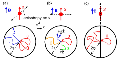
Figure 1: Sketch of the parameter space $\mathcal{M}$ (in angle-axis representation) for a spin $S\geq 1$ with a uniaxial anisotropy axis of various orientations, and a magnetic field along $z$. The various homotopy classes of closed loops are shown and labelled by the corresponding element of the fundamental homotopy group $\pi_{1}(\mathcal{M})$. See text for details.

Let $\left|\Psi_{0}^{n}\right\rangle$ (with $n=1,2,\ldots$) be the normalized eigenstates of $H_{0}$, of energies $E_{n}$. For a general rotation $\mathbf{R}$, we choose as basis functions the rotated eigenstates, $\left|\Psi_{\mathbf{R}}^{n}\right\rangle\equiv U_{\mathbf{R}}\left|\Psi_{0}^{n}\right\rangle,$ with energies $E_{n}(\mathbf{R})=E_{n}$, independent of $\mathbf{R}$. From now on, we shall restrain our discussion to the case of non-degenerate levels $E_{n}$ (abelian case). Note that $H_{\mathbf{R}}=H_{0}$ does not imply $\left|\Psi_{\mathbf{R}}^{n}\right\rangle=\left|\Psi_{0}^{n}\right\rangle$ but only $\left|\Psi_{\mathbf{R}}^{n}\right\rangle=\mathrm{e}^{-\mathrm{i}\alpha_{\mathbf{R}}^{n}}\left|\Psi_{0}^{n}\right\rangle$; this multivaluedness of the basis functions requires particular care.

Berry Berry1984 pointed out that for a system satisfying $\left|\Psi(t=0)\right\rangle=\left|\Psi_{0}^{n}\right\rangle$ adiabatically (i.e., in a time $T\gg\hbar/|E_{m}-E_{n}|$, $\forall\ m\neq n$) transported along the closed circuit $\mathcal{C}$, the wave function at time $T$ (after closing the circuit) is given by $\left|\Psi(T)\right\rangle=\mathrm{e}^{\mathrm{i}\left[\delta_{n}+\gamma_{n}(\mathcal{C})\right]}\left|\Psi_{0}^{n}\right\rangle,$ where $\delta_{n}\equiv-{\hbar}^{-1}\int_{0}^{T}E_{n}(\mathbf{R}(t))\,\mathrm{d}t=-E_{n}T/{\hbar}$ is the dynamical phase and $\gamma_{n}(\mathcal{C})\equiv\mathrm{i}\int_{\mathcal{C}}\left\langle\Psi_{n}(\mathbf{R})|\partial_{\mathbf{R}}\Psi_{n}(\mathbf{R})\right\rangle\cdot\mathrm{d}\mathbf{R}-\alpha^{n}_{\mathbf{R}(T)}$ is the Berry phase (independent of $T$ and depending only on the circuit $\mathcal{C}$), of interest here. Note that the last term, in the above equation, is due to the multivaluedness of the basis functions and was absent in the original paper of Berry Berry1984 , where a single-valued basis was considered.

Simple algebra then yields $\gamma_{n}(\mathcal{C})=\int_{\mathcal{C}}\mathbf{A}^{n}_{\mathbf{R}}\cdot\mathrm{d}\mathbf{R}-\mathrm{i}\ln\left[\left\langle\Psi_{0}^{n}\right|U_{\mathbf{R}(T)}\left|\Psi_{0}^{n}\right\rangle\right],$ with $\mathbf{A}^{n}_{\mathbf{R}}\equiv\left\langle\Psi^{n}_{0}\right|\mathbf{A}_{\mathbf{R}}\left|\Psi^{n}_{0}\right\rangle,$ and $\mathbf{A}_{\mathbf{R}}\equiv\mathrm{i}\left(U_{\mathbf{R}}\right)^{-1}\left(\partial_{\mathbf{R}}U_{\mathbf{R}}\right).$ One then obtains the components of $\mathbf{A}$: $A_{\varphi}=J_{z}(\cos\theta-1)-\sin\theta\left[J_{x}\cos(\beta-\varphi)-J_{y}\sin(\beta-\varphi)\right]$, $A_{\theta}=J_{x}\sin(\beta-\varphi)+J_{y}\cos(\beta-\varphi)$, $A_{\beta}=J_{z}$. So far, we have not specified any particular choice for the cartesian axes. When calculating $\gamma_{n}(\mathcal{C})$, it is convenient to choose the $z$-axis along the expectation value of $\mathbf{J}$ for the state $\left|\Psi^{n}_{0}\right\rangle$, i.e., $\hat{\mathbf{z}}_{n}\equiv{\mathbf{J}_{n}}/{J_{n}}$, with $\mathbf{J}_{n}\equiv\left\langle\Psi^{n}_{0}\right|\mathbf{J}\left|\Psi^{n}_{0}\right\rangle$ and $J_{n}\equiv\left\|\mathbf{J}_{n}\right\|$. Note that in the most general situation, $J_{n}$ is not a multiple of $1/2$ and that the $z$-axes defined in this way may be different for different states $n$ and $n^{\prime}$; if $J_{n}=0$, the choice of $\hat{\mathbf{z}}_{n}$ is indifferent. With this choice, one immediately gets $A_{\varphi}^{n}=J_{n}\cos(\theta_{n}-1)$, $A_{\theta}^{n}=0$, $A_{\beta}^{n}=J_{n},$ where the $n$ indices on the Euler angles remind that they are defined here with respect to a $n$-dependent $z$-axis $\hat{\mathbf{z}}_{n}$.

We now consider the last term of the Berry phase. Since $\mathbf{R}(T)$ belongs to the symmetry group of $H_{0}$, it must leave $\mathbf{J}_{n}$ invariant, so that $\theta_{n}(T)=0$; therefore $U_{\mathbf{R}(T)}=\mathrm{e}^{-\mathrm{i}\beta_{n}(\mathcal{C})J_{z}}$, where $\beta_{n}(\mathcal{C})\equiv\int_{\mathcal{C}}\mathrm{d}\beta_{n}$ is the total twist angle of the $x$- and $y$-axes around $\hat{\mathbf{z}}_{n}$. If $\hat{\mathbf{z}}_{n}$ is a symmetry axis of order $q$, we must have $\beta_{n}(\mathcal{C})=p_{n}(\mathcal{C})\,2\pi/q$, with $p_{n}(\mathcal{C})\in\mathbb{Z}$. The state $|\Psi_{0}^{n}\rangle$ may be expanded in terms of the eigenstates $|M;\hat{\mathbf{z}}_{n}\rangle$ of $J_{z}$ with quantum number $M$ (for the $z$-axis along $\hat{\mathbf{z}}_{n}$), i.e., $|\Psi_{0}^{n}\rangle\equiv\sum_{M}a_{M}^{n}|M;\hat{\mathbf{z}}_{n}\rangle.$ Let $M_{n}$ be the largest value of $M$ for which $a_{M}^{n}\neq 0$; one can easily see that the only values of $M$ for which $a_{M}^{n}\neq 0$ are of the form $M_{n}-rq$, with $r\in\mathbb{N}$, so that $\alpha^{n}_{\mathbf{R}(T)}=M_{n}\,\beta_{n}(\mathcal{C})\ \mathrm{mod}\ 2\pi$. Putting everything together, one finally obtains

$$\gamma_{n}(\mathcal{C})\!=-J_{n}\,\Omega_{n}(\mathcal{C})-\left(M_{n}\!-\!J_{n}\right)\frac{2\pi}{q}\,p_{n}(\mathcal{C})\ \,\mathrm{mod}\,2\pi,$$ (1)

where $\Omega_{n}(\mathcal{C})\equiv\int_{\mathcal{C}}\left(1-\cos\theta_{n}\right)\,\mathrm{d}\varphi_{n}$ is the (oriented) solid angle of the curve described by $\hat{\mathbf{z}}_{n}(\mathbf{R})$. Equation (1) is the central result of this paper. It is in fact a fairly general theorem, applying a broad class of systems, as it relies only on the properties of rotations, independently of any specific detail of the Hamiltonian.

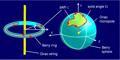
Figure 2: Schematic representation of a circuit $\mathcal{C}$ on the Berry sphere with a Dirac monopole at its center, and on the Berry ring threaded by a Dirac string. In the case depicted here, the winding number $p_{n}(\mathcal{C})$ equals zero.

The physical interpretation is as follows. A given rotation $\mathbf{R}$ is represented by a point of polar coordinates $(\varphi_{n},\theta_{n})$ on a sphere (hereafter called the Berry sphere) giving the orientation of $\hat{\mathbf{z}}_{n}(\mathbf{R})$, and by a point on a ring (hereafter called the Berry ring), with angular coordinate $q\beta_{n}$ (describing the twist of the $x$- and $y$-axes around $\hat{\mathbf{z}}_{n}(\mathbf{R})$); the winding number $p_{n}(\mathcal{C})$ of the circuit $\mathcal{C}$ around the Dirac string is a topological invariant of $\mathcal{C}$ (mod $2q$). A Dirac monopole of strength $-J_{n}$ is positioned at the center of the sphere, whereas the ring is threaded by a Dirac string carrying a flux equal to $-2\pi(M_{n}-J_{n})/q$. The Berry phase for a given circuit $\mathcal{C}$ is then given by the sum of the fluxes through $\mathcal{C}$ due to the Dirac monopole at the center of the Berry sphere and to the Dirac string threading the Berry ring, as depicted schematically on Fig. 2.

The contribution of the Dirac monopole is proportional to the solid angle $\Omega_{n}(\mathcal{C})$, which is a geometric property of the circuit $\mathcal{C}$, and may be called the geometric Berry phase. The contribution of the Dirac string is proportional to the winding number $p_{n}(\mathcal{C})$ of the circuit $\mathcal{C}$ around the Dirac string, and may be called the topological Berry phase.

The latter contribution constitutes a spin analogue of the Aharonov-Bohm effect Aharonov1959 . The analogy, however is not one-to-one, since the topology of the parameter space in the present case ($\mathcal{M}=\mathbb{R}P^{3}/\mathbb{Z}_{q}$, $\pi_{1}(M)=Z_{2q}$) differs from the one of the Aharonov-Bohm effect ($\mathcal{M}=S^{1}$, $\pi_{1}(M)=Z$). This is related to the fact that a solid angle is defined modulo $4\pi$: writing $p_{n}(\mathcal{C})=2qk_{n}(\mathcal{C})+r_{n}(\mathcal{C})$ with $r_{n}(\mathcal{C})$ and $k_{n}(\mathcal{C})$ integers, Eq. (1) may be rewritten as $\gamma_{n}(\mathcal{C})=-J_{n}\,\left[\Omega_{n}(\mathcal{C})-4\pi k_{n}(\mathcal{C})\right]-\left(M_{n}\!-\!J_{n}\right)\frac{2\pi}{q}\,r_{n}(\mathcal{C})\ \,\mathrm{mod}\ 2\pi$.

The Dirac monopole giving rise to the geometric Berry phase is generally non-quantized; the deviation from exact quantization, $M_{n}-J_{n}$, is a measure of the effect of anisotropy for $|\Psi_{0}^{n}\rangle$. This clearly illustrates the above discussion on the interplay of charge quantization and spacial isotropy. The topological Berry phase due to the Dirac string obtained here constitutes a novel effect that appears only for anisotropic systems.

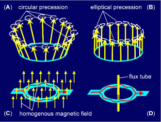
Figure 3: Illustration of the analogy between (A) the geometric Berry phase of magnons on a ring due to a texture of the magnetization and (C) the (geometric) Aharonov-Bohm effect in a homogenous field, contrasted with the analogy between (B) the topological Berry phase of magnons on a uniformly magnetized ring due to the magnetic anisotropy and (D) the “true” (topological) Aharonov-Bohm effect due to the vector potential of a flux tube.

Let us now consider how the geometric and topological Berry phases could be probed experimentally. The present theory most directly applies to nuclear or electronic spin systems in an anisotropic environment. The simplest way of probing the Berry is to repeat periodically the circuit $\mathcal{C}$ at a frequency $\omega_{\mathcal{C}}/(2\pi)$ (with $\hbar\omega_{\mathcal{C}}\ll|E_{m}-E_{n}|$, $\forall\ m\neq n$). The Berry phase will therefore increase linearly in time, which means that the energy of the state $n$ will be shifted by an amount $\Delta E_{n}=-\hbar\omega_{\mathcal{C}}\,\gamma_{n}(\mathcal{C})/(2\pi)$. These frequency shifts would be measurable as a shift $\Delta\omega=\omega_{\mathcal{C}}\,(\gamma_{n}(\mathcal{C})-\gamma_{n^{\prime}}(\mathcal{C}))/(2\pi)$ of the magnetic resonance line corresponding to transitions between the states $n$ and $n^{\prime}$. By taking suitably chosen circuits $\mathcal{C}$ one can investigate the geometric and adiabatic Berry phases separately.

In particular, by choosing a circuit that is just a rotation of $2\pi/q$ around $\hat{\mathbf{z}}_{n}$ (which is also the simplest experiment), only the topological Berry phase is probed. For nuclear spins, this is simply achieved by spinning the sample, a standard technique in nuclear magnetic resonance that was successfully applied to study both the abelian and non-abelian (geometric) Berry phases of ${}^{35}\!$Cl nuclei ($S=3/2$) Tycko1987 ; Zwanziger1990 . The simplest case is for a single spin $S\geq 1$ with Hamiltonian $H_{0}=-BS_{z}+K{S_{x}}^{2}$ (case (b) on Fig. 1). Taking $\mathcal{C}$ as a rotation of $+\pi$ around the $z$-axis, one easily calculates the Berry phase: $\gamma_{1}=-\gamma_{-1}=-\pi[1-b/\sqrt{1+b^{2}}]$, $\gamma_{0}=0$, for $S=1$, and $\gamma_{3/2}=-\gamma_{-1/2}=-\pi[1-(b+1)/\sqrt{(b+1)^{2}+3}]$, $\gamma_{1/2}=-\gamma_{-3/2}=-\pi[1-(b-1)/\sqrt{(b-1)^{2}+3}]$, for $S=3/2$, where $b\equiv 2B/K$ and where the states are labelled by the (quantized) value of $S_{z}$ obtained in the limit $K\rightarrow 0$.

For electronic spins, sample spinning is not a realistic approach. The Berry phase can nevertheless be investigated by applying the magnetic field at some angle $\theta_{B}$ with respect to the anisotropy axis (case (a) in Fig. 1), and by rotating the field on a cone of angle $\theta_{B}$ around the anisotropy axis, which can be conveniently done experimentally. The Berry phase obtained in that case contains both a geometric and a topological contribution.

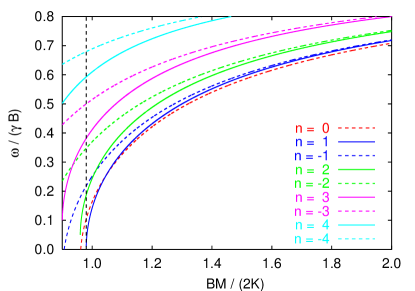
Figure 4: Magnon spectrum of a ferromagnetic ring of radius $R$, with exchange stiffness $A$ and tangential easy-axis anisotropy $K=\pi M^{2}$, in a uniform perpendicular magnetic field $B$, for a typical value $4KR^{2}/A=200$. Solid and dashed lines correspond to modes with counterclockwise and clockwise group velocities, respectively. The vertical dashed line gives the critical field for stability of the state with uniform vertical magnetization.

The Berry phase may also influence the properties of magnons. For example, it has been recently indicated that the geometric Berry phase due to a non-coplanar texture of the magnetization of a ferromagnetic ring (see Fig. 3A) would affect the dispersion of magnons (lifting the degeneracy of clockwise and anticlockwise propagating magnons), and generate some equilibrium spin currents Schutz2003 . In this study, however, the effect of magnetic anisotropy was ignored (in a classical picture, this correspond to a circular precession of the magnetization), so that the resulting Berry phase associated with the propagation of a magnon around the ring is merely that of a quantized monopole, and does not include the topological Berry phase due to a non-quantized Dirac string. The geometric Berry phase obtained in this case is analogous to the geometric (i.e., dependent on the particular geometry of electron trajectories, because of the finite width of the ring’s arms) Aharonov-Bohm effect for a ring in a homogenous magnetic field, as depicted schematically on Fig. 3C. Since magnons have a spin $S=1$, they may be subject to magnetic anisotropy. If one properly incorporates the effect of magnetic anisotropy, then the topological Berry phase gives rise to new effects. For example, if one considers a magnetic ring uniformly magnetized along the ring axis, and with some magnetic anisotropy giving a tangentially oriented easy-magnetization axis, then the precession of the magnetization (in a classical picture) has an elliptical polarization whose large axis is tangential to the ring and makes a turn of $2\pi$ around the ring (this corresponds to a winding number $p(\mathcal{C})=2$), as depicted schematically on Fig. 3B, so that a topological Berry phase is generated by the anisotropy; the degree of ellipticity, and hence the topological Berry phase, can be conveniently controlled by means of an external field parallel to the ring axis. The latter situation is analogous (except for the difference discussed earlier) to the “true” (i.e., topological) Aharonov-Bohm effect, in which the flux threading the ring is concentrated in a flux tube, the ring itself being in a field-free region (see Fig. 3D). The required anisotropy would be easily obtained as a consequence of shape (dipolar) anisotropy, if one takes a magnetic ring approximately as thick as wide. The topological Berry phase would manifest as a splitting of magnon spectrum, lifting the degeneracy between clockwise and anticlockwise propagating magnons, an effect that could be observed rather easily. A detailed account of the effect of Berry phase on magnons will be given elsewhere Dugaev2004 ; I give below, without further details, the results for the magnon spectrum of a ring of radius $R$ with exchange stiffness $A$ and (dipolar) magnetic anisotropy $K=\pi M^{2}$, in a perpendicular field $B$ sufficiently large to homogenously magnetize the ring along its axis (see Fig. 3B). I consider a typical ferromagnetic ring (Ni ring of radius $R\simeq 75$ nm, width $w\simeq 20$ nm, and thickness $h\simeq 20$ nm); the ring is characterized by the dimensionless parameter $4KR^{2}/A\simeq 200$. The calculated magnon spectrum is shown on Fig. 4, where the lifting of the degeneracy between states with anticlockwise ($n>0$) and clockwise ($n<0$) group velocity due to the topological Berry phase appears very clearly.

I am grateful to V.K. Dugaev, C. Lacroix, and B. Canals for intensive discussions throughout the elaboration process of this work. This work was partly supported by the BMBF (Grant No. 01BM924).

References

- (1) P.A.M. Dirac, Proc. Roy. Soc. London A 133, 60 (1931); Phys. Rev. 74, 817 (1948).
- (2) Y. Aharonov and D. Bohm, Phys. Rev. 115, 485 (1959).
- (3) J. Baumann et al., Phys. Rev. D 37, 3107 (1988).
- (4) M.V. Berry, Proc. R. Soc. London A 392, 45 (1984).
- (5) R. Tycko, Phys. Rev. Lett. 58, 2281 (1987).
- (6) J.W. Zwanziger et al., Phys. Rev. A 42, 3107 (1990).
- (7) F. Schütz et al., Phys. Rev. Lett. 91, 017205 (2003).
- (8) V.K. Dugaev, P. Bruno, et al., to be published.