Diffusivity and configurational entropy maxima in short range attractive colloids

Abstract

We study tagged particle diffusion at large packing fractions, for a model of particles interacting with a generalized Lennard-Jones $2n$-$n$ potential, with large $n$. The resulting short-range potential mimics interactions in colloidal systems. In agreement with previous calculations for short-range potential, we observe a diffusivity maximum as a function of temperature. By studying the temperature dependence of the configurational entropy — which we evaluate with two different methods — we show that a configurational entropy maximum is observed at a temperature close to that of the diffusivity maximum. Our findings suggest a relation between dynamics and number of distinct states for short-range potentials.

In recent years, several studies have been focused on short-range attractive systems, in which the range of the attractive part of the potential is much shorter then the typical repulsive core. In nature this behavior is encountered in colloidal systems, in which the range of the attraction can be finely tuned by changing the solvent properties or the chemistry of the dispersed particles. The short length-scale of the attraction generates many unusual phenomena, (for recent reviews see for example Ref. Frenkel, 2002; Anderson and Lekkerkerker, 2002). From a thermodynamical point of view, it is now well established that the liquid-liquid coexistence becomes metastable with respect to the fluid-solid one A.P.Gast et al. (1983); Meijer and Frenkel (1991), a phenomenon which is not observed in atomic or molecular systems where the interaction is always long-ranged. Recently, theoretical, numerical and experimental studies have analyzed the dynamical properties of these systems. One of the most astonishing discoveries is that, at high density, the metastable liquid is characterized by a non-monotonic temperature ($T$) dependence of the diffusivity: dynamics slows down not only upon cooling (as is commonly observed in molecular systems), but also upon heating. The slowing down upon heating can be so intense that a novel mechanism of arrest takes place at high $T$ Sciortino (2002), creating in the same system two different glass phases: one at low $T$ called the attractive glass and one at high $T$, the repulsive glass. The former is generated by the short-range attractive part of the potential, while the latter is due to the cage effect, i.e., caging of the particle in a shell of neighbors, analogous to the hard-sphere glass. This scenario has been confirmed experimentally Mallamace et al. (2000); Pham et al. (2002); Chen et al. (2003a); Eckert and Bartsch (2002) and by numerical simulations Puertas et al. (2002); Zaccarelli et al. (2002).

The existence of a fluid phase between two glass regions suggests that the diffusion coefficient $D$ exhibits a maximum when the strength of the attraction (or the temperature) is varied along a path of constant density. Such a feature has been observed in simulations of short-range square well models. The non-monotonic behavior of $D$ has been explained in term of Mode Coupling Theory as resulting from the competition of two different localization lengths, one associated with the “hard-core” and one with the short-range attractive bond Dawson et al. (2001). In this Letter we calculate the $T$ dependence of the configurational entropy $S_{conf}$ — a measure of the number of distinct states of the system — with the aim of providing insights into the physical origin of the $D$ maximum not (a). We use two different routes to determine $S_{conf}$: the first one, based on a Potential Energy Landscape (PEL) investigation, requires an estimate of the vibrational free energy of the system close to the explored local minima of the PEL (the so-called inherent structures (IS) Stillinger and Weber (1982)); the second one uses a perturbed Hamiltonian Frenkel and Smit (2001); Coluzzi et al. (1999) and requires the mean-square distances from a given equilibrium configuration in the limit of vanishing perturbation. In both cases, the configurational entropy is calculated as a difference between total entropy (estimated via thermodynamic integration from the ideal gas state) and the vibrational entropy. In the PEL formalism, it is crucial that the interaction potential of the system is continuous, so that IS can be properly located via a steepest descent minimization of the potential energy and so that vibrational frequencies can be properly calculated. For this reason we focus on a continuous model that possesses a steep repulsion and a short-ranged attraction, and that has been proved to reproduce features of short-ranged attractive colloidal system discussed above Vliegenthart et al. (1999). The main results of the present work are: i) the presence of a diffusivity maximum on varying the temperature for the considered attractive-colloid model that confirms that origin of this phenomenon can be ascribed to the potential being short range rather then on the particular shape chosen Puertas et al. (2002); Zaccarelli et al. (2002); ii) the existence of a maximum in the $T$ dependence of $S_{conf}$ — independent of the chosen method to estimate it; iii) the fact that the temperature at which $D$ and $S_{conf}$ have a maximum nearly coincide.

The chosen model of attractive colloid is based on a generalization of the Lennard-Jones pair potential (LJ $2n$-$n$) proposed by Vliegenthart et al. Vliegenthart et al. (1999):

$$V_{LJn}(r)=4\epsilon\left[\left(\frac{\sigma}{r}\right)^{2n}-\left(\frac{\sigma}{r}\right)^{n}\right]\ .$$ (1)

Differently from the original proposition we choose an extremely large value of the exponents, i.e. $n=100$. For this value of $n$, the potential (reported in the inset of Fig. 1) provides a continuous version of the $3\%$ square-well potential, which has been extensively studied in recent years Zaccarelli et al. (2002).

We perform standard isothermal molecular dynamics using the Nosé-Hoover thermostat Frenkel and Smit (2001). The simulated system is composed of $256$ particle confined in a cubic box with periodic boundary conditions. In order to prevent crystallization we study a $50:50$ binary mixture with the following parameters: $\sigma_{AA}/\sigma_{BB}$=$1.2$, $\sigma_{AB}$=$(\sigma_{AA}+\sigma_{BB})/2$, $\epsilon_{AA}$=$\epsilon_{BB}$=$\epsilon_{AB}$. We use Lennard Jones units ($\sigma_{AA}$ for length, $\epsilon_{AA}$ for energy, $\tau$=$(m\sigma_{AA}^{2}/\epsilon_{AA})^{1/2}$ for time). We chose the Boltzmann constant $k_{B}=1$, consequently the temperature is measured in unit of $\epsilon_{AA}$. Cut and shift in the pair potential are used ($r_{cut}$=$1.4$). The time step used is $t_{0}\!=\!7\!\times\!10^{-5}$. The packing fraction investigated is $\phi$=$0.59$, corresponding to density $\rho\simeq 1.43$.

Fig. 1 shows the mean-square displacement, $r^{2}(t)$=$N^{-1}\langle[{\bf r}(t)-{\bf r}(0)]^{2}\rangle$, where ${\bf r}$ is the $3N$ vector of the coordinates, for different temperatures ranging from $T$=$0.26$ to $T$=$2.0$. Result are in agreement with previous findings based on the square-well model Zaccarelli et al. (2002): at high $T$ there is a well defined plateau at about $r^{2}$=$2\!\times\!10^{-2}$, while at low $T$ the plateau disappears and one observes a transient sub-diffusive regime before the diffusive one. It is worth noting that the value of $r^{2}\!\sim\!10^{-3}$ at the beginning of the transient regime at low $T$ corresponds to the length of the attractive well of the pair potential. Fig. 2a shows the $D$ (evaluated from the long time limit behavior of $r^{2}$ and rescaled by the quantity $D_{0}$=$\sqrt{\sigma^{2}T/m}$) as a function of $T$. One observes a maximum located at about $T_{max}=0.4$. On lowering $T$, for $T<T_{max}$, $D$ decreases quickly, as the system approaches the attractive glass line (almost horizontal in the $\phi-T$ plane). On increasing $T$, for $T>T_{max}$, $D$ decreases smoothly, consistent with the observation that the repulsive glass line is almost vertical in the $\phi-T$ phase diagram.

In analogy with recent studies for atomic and molecular liquids, one can ask if the $T$ dependence of $D$ close to arrested states is correlated to the $T$ dependence of the $S_{conf}$, as, for example, in the well known Adam-Gibbs proposition Adams and Gibbs (1958). In the case of short-range models, a test of the correlation between $D$ and $S_{conf}$ can be exploited in a more direct way, capitalizing on the presence of the $D$-extremum at $T=T_{max}$. We try to answer this question, calculating the configurational entropy for our model system. To estimate $S_{conf}$, we write the total entropy as a sum of two contributions: a local vibration entropy $S_{vib}$ and a configurational entropy $S_{conf}$ that takes into account the number of distinct local states

$$S(T,\rho)=S_{conf}(T,\rho)+S_{vib}(T,\rho)\ .$$ (2)

This expression, which can be formally derived within the PEL framework Stillinger and Weber (1982) and within mean field for models of disordered $p$-spin systems Cavagna et al. (1998), is based on the idea that dynamics is described by two well separated time-scales: a fast dynamics describing local rearrangements of particles within a state (vibrations around local minima of the PEL) and a slow dynamics which accounts for the slow exploration of different states.

Eq. 2 shows that $S_{conf}$ can be calculated from the knowledge of total entropy $S$ and vibrational entropy $S_{vib}$. The total entropy $S$ can be calculated using thermodynamic integration along paths in the $T$-$\rho$ plane. Without entering in details (see Ref. Angelani et al. ), we can write, measuring entropy in units of $k_{B}$:

$$S(T,\rho)=S(T_{0},\rho)+\int_{T_{0}}^{T}\frac{dT}{T}\left(\frac{3}{2}N+\frac{\partial U}{\partial T}\right)\ ,$$ (3)

where $U$ is the potential energy, $T_{0}$ is a reference temperature ($T_{0}$=$0.4$ in our case), and $S(T_{0},\rho)$ is given by the following equation, which describes the path at constant $T_{0}$ connecting the ideal gas to the reference state $(T_{0},\rho)$,

$$S(T_{0},\rho)=S^{id}(T_{0},\rho)+\frac{U(T_{0})}{T_{0}}-\frac{1}{T_{0}}\int_{0}^{\rho}\frac{d\rho}{\rho^{2}}\ P_{ex}\ ,$$ (4)

where $S^{id}$ is the ideal gas contribution (which includes the entropy of mixing, since we are dealing with a binary mixture), and $P_{ex}$ is the excess pressure. Performing numerical simulations at $15$ different $\rho$ values from $0.036$ up to $1.434$, we estimated $P_{ex}(T_{0},\rho)$ and $U(T_{0},\rho)$, which, together with $U(T,\rho)$ allow us to calculate with sufficiently high precision the $T$ dependence of $S$. The calculation of the vibrational entropy requires some approximations. For this reason we follow two independent different calculation routes. In the PEL approach, the vibrational entropy can be calculated from the local curvature of the PEL around the explored inherent structures Stillinger and Weber (1982). In harmonic approximation, the vibrational entropy can be written as (omitting the density dependence):

$$S_{vib}^{(1)}(T)=\sum_{i=1}^{3N-3}[1-\ln(\beta\hbar\omega_{i})]\ ,$$ (5)

where $\hbar$ is the Plank’s constant, $\beta=1/k_{B}T$ and $\omega_{i}$ are the eigenfrequencies of the Hessian matrix evaluated at the inherent structure. The $T$ dependence, besides the factor $\beta$, is contained in the different properties of the local curvatures around the inherent structures explored at different temperatures (i.e. in the $T$ dependence of the $\omega_{i}$ values)La Nave et al. (2003).

Fig. 2b shows the configurational entropy per particle $S_{conf}^{(1)}/N$, calculated as the difference between total entropy in Eq. 2 and vibrational entropy $S_{vib}^{(1)}$ given by Eq. 5. The $T$ dependence shows a maximum at temperature $T_{max}^{(1)}\simeq 0.6$, slightly higher than that of diffusivity ($T_{max}$=$0.4$). The presence of the maximum is a remarkable result, indicating a close relationship between temperature dependence of diffusivity and configurational entropy, even if a quantitative coincidence of the peaks seems not to be exactly achieved. Of course, the use of the harmonic approximation deserves a few remarks: while in the simple liquid the harmonic approximation works well at sufficiently low $T$, in our case, due to the steepness of the pair potential, the harmonic approximation is expected to break down at a much lower $T$. Moreover, an estimate of the anharmonic contributions, following the techniques developed for atomic and molecular systems is not feasible in the present case, due to the strong $T$ dependence of the anharmonic energy. In order to corroborate the above finding, we calculate $S_{vib}$ using an alternative method, based on a Perturbed Hamiltonian approach Frenkel and Smit (2001); Coluzzi et al. (1999); not (b). One considers a perturbed Hamiltonian:

$$\beta H^{\prime}=\beta H+\alpha({\bf r}-{\bf r}_{0})^{2}\ ,$$ (6)

where $H$ is the original Hamiltonian, $\alpha$ is the strength of the perturbation and ${\bf r}_{0}$ is a given equilibrium reference configuration. The free energies $F(\alpha)$ of two systems with different $\alpha$ values ($\alpha_{\infty}$ and $\alpha_{0}$) are related by:

$$\beta F(\alpha_{\infty})=\beta F(\alpha_{0})+\int_{\alpha_{0}}^{\alpha_{\infty}}d\alpha^{\prime}\langle({\bf r}-{\bf r}_{0})^{2}\rangle_{\alpha^{\prime}}\ ,$$ (7)

where $\langle...\rangle_{\alpha^{\prime}}$ is the canonical average for a specified $\alpha^{\prime}$. In the large $\alpha_{\infty}\rightarrow\infty$ limit, $F(\alpha_{\infty})$ has the exact expression

$$\beta F(\alpha_{\infty})=3N\ln\lambda+\beta E_{0}+\frac{3N}{2}\ln(\alpha_{\infty}/\pi)\ ,$$ (8)

where $E_{0}$ is the potential energy of the reference configuration ${\bf r}_{0}$ and $\lambda$ is the thermal deBroglie wavelength $\lambda=(2\pi\beta\hbar^{2}/m)^{1/2}$. If a small $\alpha_{0}$ value can be chosen in such a way that the corresponding system is equivalent to the original system, but constrained to explore only the phase space of one state, the estimate of $\int_{\alpha_{0}}^{\alpha_{\infty}}d\alpha^{\prime}\langle({\bf r}-{\bf r}_{0})^{2}\rangle_{\alpha^{\prime}}$ is sufficient to evaluate the required vibrational free energy.

Writing the free energy as a sum of a potential energy term and an entropic term, $\beta F(\alpha_{0})=\beta E_{0}+3N/2-S_{vib}$, the following expression for the vibrational entropy is derived:

$$S_{vib}^{(2)}(T)=\int_{\alpha_{0}}^{\alpha_{\infty}}d\alpha^{\prime}\langle({\bf r}-{\bf r}_{0})^{2}\rangle_{\alpha^{\prime}}-\frac{3N}{2}\ln\left(\frac{\alpha_{\infty}\lambda^{2}}{\pi e}\right)\ ,$$ (9)

where $e$ is the Neper number. We use isothermal molecular dynamics with Hamiltonian $H^{\prime}$ to calculate $\langle({\bf r}-{\bf r}_{0})^{2}\rangle_{\alpha}$ at different $\alpha$ and $T$. We perform averages over $20$ different reference configurations ${\bf r}_{0}$, chosen from equilibrated configurations with unperturbed Hamiltonian $H$ at temperature $T$. Fig. 3 shows $\langle({\bf r}-{\bf r}_{0})^{2}\rangle_{\alpha}$ as a function of $\alpha$ for different $T$. The dashed line is the ($T$ independent) high $\alpha$ limit, $3/(2\alpha)$. As discussed above, one has to choose an $\alpha_{0}$ value in Eq. 9 in such a way that the system remains trapped in a given local state. While at high temperature the data are smooth and the values of $\langle({\bf r}-{\bf r}_{0})^{2}\rangle_{\alpha}$ remain well below the cage value (about $r^{2}\simeq 2\!\times\!10^{-2}$), at low $T$ the behavior is quite different: starting from high $\alpha$, we observe first an approach to a small value $r^{2}\simeq 2\!\times\!10^{-3}$ (corresponding to more or less the same behavior in the mean square displacement, even if less pronounced - see Fig. 1) and then a departure from it at smaller values of $\alpha$. We interpret the former as the vibrational motion inside the state. The full line in Fig. 3 is a guide to the eyes that extrapolates the first behavior at lower $\alpha$ for the $T$=$0.26$ case. We have then chosen as $\alpha_{0}$ in Eq. 9 a value for which the system has not yet left the line: $\alpha_{0}=5\!\times\!10^{2}$ (indicated by an arrow in Fig. 3). Although this is a feature only of the low $T$ data, we have chosen the same $\alpha_{0}$ for the estimation of $S_{vib}^{(2)}$ for all $T$, in order to obtain a coherent definition of it. The $\alpha_{\infty}$ has been fixed at $2\!\times\!10^{6}$, where $\langle({\bf r}-{\bf r}_{0})^{2}\rangle_{\alpha}$ has reached the asymptotic behavior (dashed line in Fig. 3). Fig. 2c shows the $T$ dependence of the configurational entropy per particle $S_{conf}^{(2)}/N$, calculated as the difference between total entropy and $S_{vib}^{(2)}$ not (c). Again one observes a peak, located at about $T_{max}^{(2)}\simeq 0.5$, close to that of diffusivity. We note that using the same value of $\alpha_{0}$ for all the temperatures introduces an underestimation of $S_{vib}^{(2)}$, more pronounced for the high $T$ data. This fact could have the effect of moving the peak to a lower $T$ value, approaching the peak value of the diffusivity. Although the absolute values of $S_{conf}^{(1)}$ and $S_{conf}^{(2)}$ are different, the $T$ dependence is quite similar, suggesting that the errors are mostly $T$ independent. More interestingly, in both approximations, a maximum in $S_{conf}$, not far from the $T$ at which $D$ has a maximum, is clearly detected. Since both methods give a $T$ dependence of the configurational entropy with a peak located close to that of diffusivity, our work strongly support the possibility that in short-range colloidal systems the diffusivity maximum is related to a maximum in the number of states visited by the system.

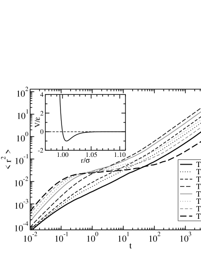
Figure 1: Mean square displacements for different temperatures (from $T$=$0.26$ to $T$=$2.0$). In the inset the pair potential LJ $2n$-$n$, with $n$=$100$.

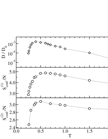
Figure 2: a) Diffusivity $D$ as a function of temperature. The value of $D$ is plotted rescaled by $D_{0}$=$\sqrt{\sigma^{2}T/m}$. b) Configurational entropy $S_{conf}^{(1)}$ per particle using Eq. 5 to estimate the vibrational entropy (PEL approach). c) $S_{conf}^{(2)}$ per particle using Eq. 9 for vibrational entropy (Perturbed Hamiltonian approach) not (c).

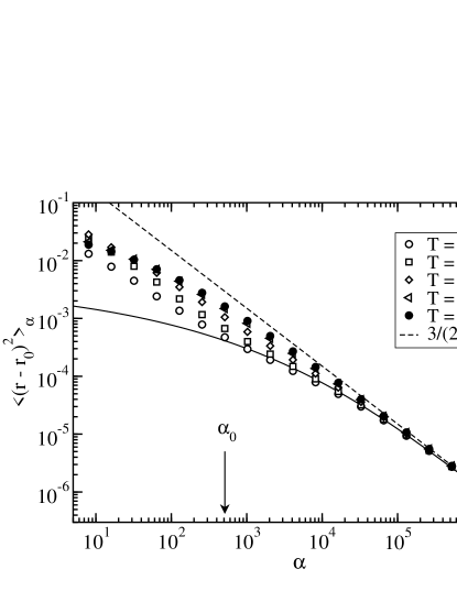
Figure 3: The quantity $\langle({\bf r}-{\bf r}_{0})^{2}\rangle_{\alpha}$ at different temperatures as a function of $\alpha$. Dashed line is the high $\alpha$ limit $3/(2\alpha)$. Full line is a guide to the eyes of the $T=0.26$ data, extrapolating the approach to a plateau with a small $r^{2}$ value. The arrow indicates the value of $\alpha_{0}$ chosen to define a state, $\alpha_{0}=5\!\times\!10^{2}$.

We thank G. Parisi for useful discussions and for suggesting the use of the perturbed Hamiltonian method to calculate the vibrational entropy. We acknowledge support from INFM Initiative Parallel Computing, and MURST COFIN2002.

References

- Frenkel (2002) D. Frenkel, Science 296, 65 (2002).
- Anderson and Lekkerkerker (2002) V. Anderson and H. Lekkerkerker, Nature 416, 811 (2002).
- A.P.Gast et al. (1983) A.P.Gast, W. Russell, and C. Hall, J. Colloid Interface Sci. 96, 1977 (1983).
- Meijer and Frenkel (1991) E. Meijer and D. Frenkel, Phys. Rev. Lett. 67, 1110 (1991).
- Sciortino (2002) F. Sciortino, Nature Materials 1, 145 (2002).
- Mallamace et al. (2000) F. Mallamace et al., Phys. Rev. Lett. 84, 5431 (2000).
- Pham et al. (2002) K. N. Pham et al., Science 296, 104 (2002); Phys. Rev. E 69, 011503 (2004).
- Chen et al. (2003a) S.-H. Chen, W.-R. Chen, and F. Mallamace, Science 300, 619 (2003a); Phys. Rev. E 68, 041402 (2003b).
- Eckert and Bartsch (2002) T. Eckert and E. Bartsch, Phys. Rev. Lett. 89, 125701 (2002); Faraday Discuss. 123, 51 (2003).
- Puertas et al. (2002) A. M. Puertas, M. Fuchs, and M. E. Cates, Phys. Rev. Lett. 88, 098301 (2002); Phys. Rev. E 67, 031406 (2003).
- Zaccarelli et al. (2002) E. Zaccarelli et al., Phys. Rev. E 66, 041402 (2002).
- Dawson et al. (2001) K. Dawson et al., Phys. Rev. E 63, 011401 (2001).
- not (a) In a previou study of a model for water Scala et al. (2000), that posses a phase diagram characterized by an iso-thermal diffussivity maximum line (as opposed to te present isochoric diffusivity maximum line), the location of the extrema did correlate with extrema. It is worth noting that in the case of water, the density maximum arises from the non spherical-features of the potential.
- Stillinger and Weber (1982) F. Stillinger and T. Weber, Phys. Rev. A 25, 978 (1982); Science 225, 983 (1984).
- Frenkel and Smit (2001) D. Frenkel and B. Smit, Understanding Molecular Simulation (Academic Press, London, 2001), 2nd ed.
- Coluzzi et al. (1999) B. Coluzzi et al., J. Chem. Phys. 111, 9039 (1999).
- Vliegenthart et al. (1999) G. A. Vliegenthart, J. Lodge, and H. N. W. Lekkerkerker, Physica A 263, 378 (1999).
- Adams and Gibbs (1958) G. Adams and J. H. Gibbs, J. Chem. Phys. 3, 139 (1958).
- Cavagna et al. (1998) A. Cavagna, I. Giardina, and G. Parisi, Phys. Rev. B 57, 11251 (1998).
- (20) L. Angelani et al., in preparation.
- La Nave et al. (2003) E. La Nave et al., J. Phys.: Condens. Matter 15, S1085 (2003).
- not (b) We note that, due to the presence of some misprints in Ref. Coluzzi et al., 1999, our formulae do not match those reported in that paper.
- not (c) A constant has been added to the , to extimate the error originated by the finite value of used. The value of has been calculated as the integral of the extrapolated line for at (see full line in Fig. 3) from to . This gives a correct estimation of for , and represnt a lower bound for the at higher .
- Scala et al. (2000) A. Scala et al., Nature 406 (2000).