Variational approach to the modulational instability

Abstract

We study the modulational stability of the nonlinear Schrödinger equation (NLS) using a time-dependent variational approach. Within this framework, we derive ordinary differential equations (ODEs) for the time evolution of the amplitude and phase of modulational perturbations. Analyzing the ensuing ODEs, we re-derive the classical modulational instability criterion. The case (relevant to applications in optics and Bose-Einstein condensation) where the coefficients of the equation are time-dependent, is also examined.

Modulational instability (MI) is a general feature of discrete as well as continuum nonlinear wave equations. This instability shows that in such settings, a specific range of wavenumbers of plane wave profiles of the form $u(x,t)\sim\exp(i(kx-\omega t))$ becomes unstable to modulations. The latter effect leads to an exponential growth of the unstable modes and eventually to delocalization (upon excitation of such wavenumbers) in momentum space. That is, in turn, equivalent to localization in position space, and hence the formation of localized, coherent solitary wave structures [1].

The realizations of this instability span a diverse set of disciplines ranging from fluid dynamics [2] (where it is usually referred to as the Benjamin-Feir instability) and nonlinear optics [3] to plasma physics [4]. One of the earliest contexts in which its significance was appreciated was the linear stability analysis of deep water waves. It was much later recognized that the conditions for MI would be significantly modified for discrete settings relevant to, for instance, the local denaturation of DNA [5] or coupled arrays of optical waveguides [6]. In the latter case, the relevant model is the discrete nonlinear Schrödinger equation (DNLS), and its MI conditions were discussed in [7]. Most recently, the MI has been recognized as responsible for dephasing and localization phenomena in the context of Bose-Einstein condensates (BEC) in the presence of an optical lattice [8, 9, 10, 11].

In this brief report, we present an alternative approach to the modulational stability of plane waves in the context of the nonlinear Schrödinger equation

$$i\psi_{t}=-\psi_{xx}-U|\psi|^{2}\psi,$$ (1)

where $\psi$ is a complex field, the subscripts denote partial derivatives with respect to the corresponding variable and $U$ is a constant prefactor (the strength of the nonlinearity). We examine MI using a time dependent variational approach (TDVA), and study the results in comparison with the standard linear stability (LS) calculations. It should be mentioned that the use of TDVA for the study of solitons at the classical [12] and even at the quantum [13] level is not novel. What distinguishes our study from these earlier ones is the use of the MI-motivated ansatz in the TDVA (see below). We also note in passing that MI and solitons from a quantum mechanical point of view have been considered in a number of references including (but not limited to) [14]. Furthermore, a similar in spirit, 3-mode approximation was systematically developed in the works of [15]. There are however a number of differences between the latter and the present approach such as e.g., our use of the variational formulation of the problem (instead of the application of the 3-mode ansatz in the dynamical equation in the context of [15]), as well as the fact that we are perturbing around an exact plane wave solution, while in the case of [15], the plane wave is an additional mode in the relevant expansion.

In the linear stability framework (see e.g., [7, 9] and references therein for relevant details), the stability of the plane waves has been examined. The latter are of the form

$$\psi(x,t)=\psi_{0}\exp\left[i\left(kx-\omega t\right)\right],$$ (2)

and constitute exact solutions of the nonlinear Schrödinger equation with a dispersion relation

$$\omega=k^{2}-U\psi_{0}^{2}.$$ (3)

Then, the MI is examined in the LS framework using the linearization

$$u(x,t)=(\psi_{0}+\epsilon c)\exp[i((kx-\omega t)+\epsilon d(x,t))]$$ (4)

and analyzing the $O(\epsilon)$ terms as

$$c(x,t)=c_{0}\exp(i\beta(x,t)),\quad d(x,t)=d_{0}\exp(i\beta(x,t)).$$ (5)

Using $\beta(x,t)=qx-\Omega t,$ the dispersion relation connecting the wavenumber $q$ and frequency $\Omega$ of the perturbation (see e.g., [1])

$$(-\Omega+2kq)^{2}=q^{2}(q^{2}-2U\psi_{0}^{2})$$ (6)

is obtained. This implies that the instability region for Eq. (1) appears for perturbation wavenumbers $q^{2}<{2U}\psi_{0}^{2}$, and in particular only for focusing nonlinearities (to which we restrict this study).

We now attempt to identify the interval of unstable wavenumbers by means of the TDVA. In particular, we start from the Lagrangian L

$$L=\int_{-\infty}^{\infty}\left[\frac{i}{2}\left(\psi^{\ast}\psi_{t}-\psi\psi_{t}^{\ast}\right)-|\psi_{x}|^{2}+\frac{U}{2}|\psi|^{4}\right]~{}dx,$$ (7)

and consider a modulation of the plane wave of the form

$$\psi=[\psi_{0}+a(t)\exp(i\phi_{a}(t))\exp(iqx)+b(t)\exp(i\phi_{b}(t))\exp(-iqx)]\exp\left(i(kx-\omega t)\right).$$ (8)

However, instead of considering the modulation directly at the level of the equation, the variation of our approach is that we use the modulational ansatz in the Lagrangian. This constitutes the basic novel ingredient of this variational-type approach to the modulational instability.

Here we consider an annular (1-dimensional) geometry, which imposes periodic boundary conditions on the wavefunction $\psi(x)$ and integration limits $0\leq x<2\pi$ in Eq. (7). This results in the quantization of the wavenumbers $k,q=0,\pm 1,\pm 2,...$. However, it is clear that our results can be easily generalized to the case of an infinite, open system and to higher dimensions.

After substitution of Eq. (8) into Eq. (7), we obtain the variational Lagrangian

$$L= \pi[-2(a^{2}\dot{\phi}_{a}+b^{2}\dot{\phi}_{b})+2(U\psi_{0}^{2}-q^{2})(a^{2}+b^{2})-U\psi_{0}^{4}-4qk(a^{2}-b^{2})+4U\psi_{0}^{2}ab\cos(\phi_{a}+\phi_{b})$$ (10)

$$+U(a^{4}+b^{4}+4a^{2}b^{2})].$$

It is clear from this Lagrangian that the pair $\phi_{a}(t),\phi_{b}(t)$ can be interpreted as the generalized coordinates of the system, while $A(t)=2a^{2}(t),B(t)=2b^{2}(t)$ are the corresponding momenta. In particular, the pairs $A(t),\phi_{a}(t)$ and $B(t),\phi_{b}(t)$ are canonically conjugate with respect to the effective Hamiltonian

$$H_{eff}=(U\psi_{0}^{2}-q^{2})(A+B)-2qk(A-B)+2U\psi_{0}^{2}\sqrt{AB}\cos(\phi_{a}+\phi_{b})+{U\over 4}(A^{2}+B^{2}+4AB),$$ (11)

which is an exact integral of motion on the subspace spanned by Eq. (8).

The Lagrangian equations of motion are:

$$\frac{d}{dt}\frac{\partial L}{\partial\dot{a}} = \frac{\partial L}{\partial a}\Rightarrow a\dot{\phi}_{a}=C_{1}a+C_{2}b\cos(\phi_{a}+\phi_{b})+Ua(a^{2}+2b^{2})$$ (12)

$$\frac{d}{dt}\frac{\partial L}{\partial\dot{\phi}_{a}} = \frac{\partial L}{\partial\phi_{a}}\Rightarrow\dot{a}=C_{2}b\sin(\phi_{a}+\phi_{b})$$ (13)

$$\frac{d}{dt}\frac{\partial L}{\partial\dot{b}} = \frac{\partial L}{\partial b}\Rightarrow b\dot{\phi}_{b}=C_{3}b+C_{2}a\cos(\phi_{a}+\phi_{b})+Ub(b^{2}+2a^{2})$$ (14)

$$\frac{d}{dt}\frac{\partial L}{\partial\dot{\phi}_{b}} = \frac{\partial L}{\partial\phi_{b}}\Rightarrow\dot{b}=C_{2}a\sin(\phi_{a}+\phi_{b}),$$ (15)

where $C_{1}=U\psi_{0}^{2}-q^{2}-2qk$, $C_{2}=U\psi_{0}^{2}$, and $C_{3}=U\psi_{0}^{2}-q^{2}+2qk$ are constant prefactors.

If we now keep all terms to O$(a)$ in Eqs. (12)-(15) [which is consistent with an approximation linear in $a$], we obtain

$$a = b$$ (16)

$$\dot{a} = C_{2}a\sin(\phi)$$ (17)

$$\dot{\phi} = (C_{1}+C_{3})+2C_{2}\cos(\phi),$$ (18)

where $\phi=\phi_{a}+\phi_{b}$. The latter equation has the solution

$$\phi(t)=2\arctan\left[\frac{\sqrt{(2U\psi_{0}^{2}-q^{2})q^{2}}}{q^{2}}\tanh\left(\sqrt{(2U\psi_{0}^{2}-q^{2})q^{2}}t\right)\right].$$ (19)

Two different cases arise here, corresponding respectively to whether the instability criterion is satisfied or not. Namely, when $2U\psi_{0}^{2}-q^{2}<0$ the solution of Eq. (17) is

$$a(t)\sim\sqrt{1-\frac{2U\psi_{0}^{2}}{q^{2}}\sin\left(\sqrt{(q^{2}-2U\psi_{0}^{2})q^{2}}t\right)^{2}},$$ (20)

while when $2U\psi_{0}^{2}-q^{2}>0$ the solution of Eq.(17) is

$$a(t)\sim\sqrt{1+\frac{2U\psi_{0}^{2}}{q^{2}}\sinh\left(\sqrt{(2U\psi_{0}^{2}-q^{2})q^{2}}t\right)^{2}}.$$ (21)

The solutions signal the appearance of the modulational instability when the threshold condition $q^{2}=2U\psi_{0}^{2}$ is crossed (passing from higher to lower perturbation wavenumbers). This is also clearly shown in the time evolution of $a(t)$ in accordance with Eqs. (20)-(21) also shown in Fig. 1 in the case of $q=2$ for $\frac{2U\psi_{0}^{2}}{q^{2}}=0.2$ (see the left panel of Fig. 1) and $\frac{2U\psi_{0}^{2}}{q^{2}}=1.2$ (see the right panel of Fig. 1).

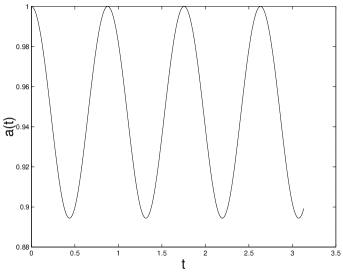
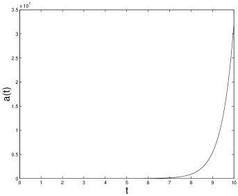
FIG. 1.: The left panel shows the (stable oscillatory) time evolution of $a(t)$ for the case $\frac{2U\psi_{0}^{2}}{q^{2}}=0.2$, in accordance with Eq. (20). The right panel shows the (unstable, exponentially growing) time evolution of $a(t)$ for the case of $\frac{2U\psi_{0}^{2}}{q^{2}}=1.2$, in accordance with Eq. (21).

An alternative, more intuitive way to appreciate the linear stability result from a dynamical systems viewpoint. This consists of reducing Eqs. (12)-(15) to a one degree of freedom setting with an effective potential energy landscape whose (parametric) variation will elucidate the instability. Along these lines, using $A(t=0)=0$ in (without loss of generality) in Eq. (10) and $A(t)=B(t)$ (from Eqs. (13) and (15)) in Eq. (11), we have:

$$\tilde{H}=\pi\left[2(U\psi_{0}^{2}-q^{2})A+\frac{3}{2}UA^{2}+2U\psi_{0}^{2}A\cos{\phi}\right]=0.$$ (22)

Eliminitating $\phi$ from Eqs. (13) and (22) for $A(0)=0$, we obtain the “energy equation” for $A$

$$\frac{1}{2}\dot{A}^{2}+V_{eff}=0,$$ (23)

where the effective potential $V_{eff}(A)$ is of the form:

$$V_{eff}(A)=2q^{2}(q^{2}-2U\psi_{0}^{2})A^{2}+3U(U\psi_{0}^{2}-q^{2})A^{3}+\frac{9}{8}U^{2}A^{4}$$ (24)

One can then examine the stability of the effective potential by evaluating its curvature at $A=0$. We thus obtain $V_{eff}^{\prime\prime}(A)|_{A=0}=4q^{2}(q^{2}-2U\psi_{0}^{2})$ and hence the potential will be convex (and therefore the dynamics will be stable) for $q^{2}>2U\psi_{0}^{2}$, while it will be concave (and the dynamics unstable) for $q^{2}<2U\psi_{0}^{2}$. Hence in this case also, we retrieve the modulational stability criterion. The effective potential is shown for the modulationally stable, unstable and marginal case in Fig. 2.

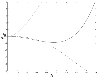
FIG. 2.: The effective potential of Eq. (24) is shown for as a function of $A$ for $U=\psi_{0}=1$ and three different values of $q$: $q=1$ (modulationally unstable; solid line), $q=\sqrt{2}$ (at the threshold; dashed line) and $q=2$ (modulationally stable; dash-dotted line).

Now we turn to a more interesting case, where the coefficient of the dispersion term, as well as the coefficient of the nonlinear term in Eq. (1) are temporally modulated, namely we examine the equation

$$i\psi_{t}=-D(t)\psi_{xx}-U(t)|\psi|^{2}\psi.$$ (25)

Our aim is to derive the modulational stability equation via the TDVA, for general $D(t)$ and $U(t)$. It is interesting to note that this equation has become of increasing importance in the past decade due to applications both in optics and also, more recently, in soft condensed-matter physics. In particular, in optics, the case of $D(t)$ periodic and $U(t)$ constant is of relevance in the context of the so-called dispersion management. The latter is based on periodic alternation of fibers with opposite signs of the group-velocity dispersion [16]. We note in passing that in this application time $t$ is, in reality, the propagation distance (i.e., space), while $x$ corresponds to a retarded time variable. An alternative setting where $D(t)$ is constant, but $U(t)$ can be temporally modulated (via a Feshbach resonance, i.e., an external magnetic field; see e.g., [17]) can be found in Bose-Einstein condensation. In the latter setting, there has been an explosion of interest recently in time dependent scattering length and its effect on patterns, coherent structures and collapse thereof (a number of very recent references can be found in [18, 19, 20, 21]. While our primary motivation in considering MI through the TDVA in Eq. (25) principally stems from this recently explored experimental potential in Bose-Einstein condensates, we should note that this type of problem was investigated earlier in nonlinear optics, see e.g., [22].

We consider the perturbation of the form

$$\psi=\psi_{1}\left[1+w(t)\cos(qx)\right]$$ (26)

to the plane wave solution $\psi_{1}=e^{i(-k^{2}\int_{0}^{t}D(s)ds+\int_{0}^{t}U(s)ds+kx)}$. Notice that in Eq. (26), we are using for simplicity a variant of the ansatz of Eq. (8), with $a=b$, $\phi_{a}=\phi_{b}$ and (without loss of generality) $\psi_{0}=1$. Following the same procedure as above, we can obtain the stability equations for $w=w_{r}+iw_{i}$:

$$\dot{w}_{r}=q^{2}D(t)w_{i}-\frac{3}{4}U(t)\left(w_{i}^{3}+w_{i}w_{r}^{2}\right)$$ (27)

$$\dot{w}_{i}=-\left[q^{2}D(t)-2U(t)\right]w_{r}+\frac{3}{4}U(t)\left(w_{r}^{3}+w_{r}w_{i}^{2}\right)$$ (28)

Hence, at the linear level, we can derive the following stability equation

$$\ddot{w}_{r}=\frac{\dot{D}(t)}{D(t)}\dot{w}_{r}-q^{2}D(t)\left[q^{2}D(t)-2U(t)\right]w_{r}$$ (29)

By determining the windows of stability of the ordinary differential equation of (29), the modulational stability of Eq. (25) is determined. It is further worth noting that for $D(t)$ constant and $U(t)$ time-periodic, Eq. (29) falls into Eq. (2) of [21] and becomes Hill’s equation for which many stability results are known in the mathematical literature [23]. Furthermore, in the case of $U(t)=1+2\alpha\cos(\omega t)$, Eq. (29) falls into Eq. (2) of [18] and the resulting equation is of the Mathieu type for which explicit stability windows can be computed (for details see [18] and references therein). It then becomes naturally an interesting problem in mathematical physics to determine the stability of Eq. (29) for more general cases (e.g., with both coefficients periodically varying etc.).

In this brief report, we have revisited the modulational instability from a different point of view, namely a variational one. We have used this dynamical systems’ type approach to derive the Euler-Lagrange equations for the time-dependent perturbation ansatz parameters and have examined their stability for different wavenumbers of the perturbation (which affect the constants of the ensuing set of ordinary differential equations). We have retrieved, in a simple and intuitive way, the criterion for the instability. The technique has also been generalized in cases in which the coefficients of the dispersion and/or nonlinearity are temporally varying (a case which we have argued to be relevant to a variety of applications). We have found the corresponding stability condition obtaining a novel ordinary differential equation, whose special cases correspond to stability/instability criteria established previously. It would be interesting to extend the considerations of this method (which seems applicable to any setting with an underlying Lagrangian/Hamiltonian structure) to contexts with explicit spatial dependence of the potential (see e.g., [9, 11]).

The support of NSF (DMS-0204585), UMass and the Clay Institute (PGK) is gratefully acknowledged. Work at Los Alamos is supported by the US DoE.

REFERENCES

- [1] C. Sulem and P.L. Sulem, The Nonlinear Schrödinger Equation, Springer-Verlag (New York, 1999).
- [2] T.B. Benjamin and J.E. Feir, J. Fluid. Mech. 27, 417 (1967).
- [3] L.A. Ostrovskii, Sov. Phys. JETP 24, 797 (1969).
- [4] T. Taniuti and H. Washimi, Phys. Rev. Lett. 21, 209 (1968); A. Hasegawa, Phys. Rev. Lett. 24, 1165 (1970).
- [5] M. Peyrard, T. Dauxois, H. Hoyet and C.R. Willis, Physica 68D, 104 (1993).
- [6] R. Morandotti, U. Peschel, J.S. Aitchison, H.S. Eisenberg and Y. Silberberg, Phys. Rev. Lett. 83, 2726 (1999).
- [7] Yu.S. Kivshar and M. Peyrard, Phys. Rev. A 46, 3198 (1992).
- [8] B. Wu and Q. Niu, Phys. Rev. A 64, 061603(R) (2001).
- [9] A. Smerzi, A. Trombettoni, P.G. Kevrekidis and A.R. Bishop, Phys. Rev. Lett., 89, 170402 (2002).
- [10] V. V. Konotop, and M. Salerno, Phys. Rev. A65, 021602 (2002).
- [11] F. S. Cataliotti et al., New Journal of Physics 5, 71 (2003).
- [12] B.A. Malomed, Prog. Opt. 43, 71 (2002).
- [13] B. Crosignani, P. Di Port and A. Treppiedi, Quantum Semiclass. Opt. 7, 73 (1995).
- [14] T.A.B. Kennedy, Phys. Rev. A 44, 2113 (1991); S.J. Carter, P.D. Drummond, M.D. Reid and R.M. Shelby, Phys. Rev. Lett. 58, 1841 (1987); P.D. Drummond, S.J. Carter and R.M. Shelby, Opt. Lett. 14, 373 (1989); H. Haus and Y. Lai, J. Opt. Soc. Am. B 7, 386 (1990); H.P. Thacker, Rev. Mod. Phys. 53, 253 (1981).
- [15] S. Trillo and S. Wabnitz, Opt. Lett. 16, 986 (1991); G. Cappellini and S. Trillo, J. Opt. Soc. Am. B 8, 824 (1991); S. Trillo and S. Wabnitz, Opt. Lett. 16, 1566 (1991).
- [16] C. Kurtzke, IEEE Photon. Technol. Lett. 5, 1250 (1993); N.J. Smith et al., Electron. Lett. 32, 54 (1996); I. Gabitov and S. Turitsyn, Opt. Lett. 21, 327 (1996); N.J. Smith and N.J. Doran, Opt. Lett. 21, 570 (1996).
- [17] S. Inouye et al., Nature 392, 151 (1998); J. Stenger et al., Phys. Rev. Lett. 82, 2422 (1999).
- [18] K. Staliunas, S. Longhi and G. J. de Valcárcel, Phys. Rev. Lett. 89, 210406 (2002).
- [19] F.Kh. Abdullaev, E.N. Tsoy, B.A. Malomed, R.A. Kraenkel, cond-mat/0306281; F.Kh. Abdullaev, J.G. Caputo, R.A. Kraenkel, B.A. Malomed, cond-mat/0209219.
- [20] E.A. Donley et al., Nature 412, 295 (2001).
- [21] P.G. Kevrekidis, G. Theocharis, D.J. Frantzeskakis and B.A. Malomed, Phys. Rev. Lett. 90, 230401 (2003).
- [22] J. Bronski and N. Kutz, Opt.Lett. 21, 937 (1996); F.K. Abdullaev, S.A. Darmanyan, A. Kobyakov and F. Lederer. Phys.Lett.A 220, 213, (1996).
- [23] W. Magnus and S. Winkler, Hill’s Equation (Wiley, New York, 1966).