Modulational and Parametric Instabilities of the Discrete Nonlinear Schrödinger Equation

Abstract

We examine the modulational and parametric instabilities arising in a non-autonomous, discrete nonlinear Schrödinger equation setting. The principal motivation for our study stems from the dynamics of Bose-Einstein condensates trapped in a deep optical lattice. We find that under periodic variations of the heights of the interwell barriers (or equivalently of the scattering length), additionally to the modulational instability, a window of parametric instability becomes available to the system. We explore this instability through multiple-scale analysis and identify it numerically. Its principal dynamical characteristic is that, typically, it develops over much larger times than the modulational instability, a feature that is qualitatively justified by comparison of the corresponding instability growth rates.

I Introduction

The modulational instability (MI) is a general feature of discrete as well as continuum nonlinear wave equations. For this instability, a specific range of wavenumbers of plane wave profiles of the form $u(x,t)\sim\exp(i(kx-\omega t))$ becomes unstable to modulations, leading to an exponential growth of the unstable modes and eventually to delocalization (upon excitation of such wavenumbers) in momentum space. That is equivalent to localization in position space, and hence the formation of localized, coherent solitary wave structures [1].

The realizations of this instability span a diverse set of disciplines ranging from fluid dynamics [2] (where it is usually referred to as the Benjamin-Feir instability) and nonlinear optics [3] to plasma physics [4]. One of the earliest contexts in which its significance was appreciated was the linear stability analysis of deep water waves. It was much later recognized that the conditions for MI would be significantly modified for discrete settings relevant to, for instance, the local denaturation of DNA [5] or coupled arrays of optical waveguides [6, 7]. In the latter case, a relevant model is the discrete nonlinear Schrödinger equation (DNLS), and its MI conditions were discussed in [8]. Most recently, the MI has been recognized as responsible for dephasing and localization phenomena in the context of Bose-Einstein condensates (BEC) in the presence of an optical lattice i.e., a sinusoidal external potential [9, 10, 11, 12].

In the context of BECs which are among the principal motivations of this work, another interesting possibility arises. For a “deep” optical lattice (i.e., if the wells of the spatially periodic potential are well-separated and sufficiently high), it has been shown that the relevant mean field model that describes the behavior of the condensate, at $T=0$, is the discrete nonlinear Schrödinger (DNLS) equation [10, 13, 14, 15]. The optical lattice can be created by two counterpropagating laser beames forming a standing wave interference pattern.

Our interest in the present work is in introducing an explicit temporally periodic modulation in the coefficients of the DNLS and examining the instabilities that may arise (for uniform solutions). In the BEC setting, there is a number of potential realizations of such a non-autonomous DNLS equation. For instance, the heights of the interwell barriers of the optical lattice are proportional to the intensity of the lasers, and can be easily periodically modulated in time. This induces an oscillating tunneling amplitude of the condensates between adjacent wells, as well as an oscillating interaction energy of the condensates trapped in each well. An alternative possibility involves the periodic modulation of the scattering length of the interaction between the atoms via a Feshbach resonance, i.e., an external magnetic field; see e.g., [16]. The possibility of this, so-called, Feshbach resonance management (FRM) of the interaction has generated a large interest recently due its robust effect on patterns, coherent structures and its potential for avoiding collapse, see e.g., [22, 17, 18, 19, 20].

In this short communication, we revisit the modulational instability criteria in the DNLS equation (which were originally derived in [8]), but in the presence of the periodic modulation of the DNLS tunneling and interaction parameters, as motivated above. We choose the simplest possible periodic modulation (a sinusoidal variation of the atomic scattering length) and derive the modulational stability equation, which in this case becomes a modified Mathieu equation. In the absence of the periodic perturbation we recover the results of [8]. In the presence of such a term, an additional, parametric instability becomes possible. These new domains of instability appear due to parametric resonance, whenever the parameters of a system vary periodically with time. In contrast to ordinary resonance, where we have growth proportional to the time variable, here the growth is exponential, as in the case of customary modulational instability; see e.g., [21]. We implement a multiple-scale expansion to identify the instability domain boundaries and subsequently numerically examine our analytical predictions. The numerical investigations indicate that this parametric resonance sets in over much longer time scales than the modulational instability (for the same perturbation amplitude). Similar considerations for the continuum problem can be found in [22, 23].In [22] a slightly more restricted ansatz was used [$q=0$ was used in our Eq. (5) below], and in [23] it was the dispersion that was varying with time, instead of the nonlinearity strength as in our case. The continuum limit of our analytical results (modulo the relevant rescalings/adjustments) has been found to agree with the results of [22, 23].

Our presentation is structured as follows. In section II we present the mathematical framework and our analytical results. In section III we corroborate these results with numerical simulations. Finally, in section IV, we summarize our results and present our conclusions.

II Setup and Analytical Considerations

We study the discrete nonlinear Schrödinger equation in the form:

$$i\dot{\psi}_{n}=-D(t)(\psi_{n+1}+\psi_{n-1}-2\psi_{n})+a(t)|\psi_{n}|^{2}\psi_{n}+E(t)\psi_{n},$$ (1)

where the coefficients $D(t)$, $a(t)$ and $E(t)$ are time dependent. If one sets $\psi_{n}(t)=\phi_{n}(t)e^{-i\int_{0}^{t}(2D(s)+E(s))ds}$, then (1) is reduced to

$$i\dot{\phi}_{n}=-D(t)(\phi_{n+1}+\phi_{n-1})+a(t)|\phi_{n}|^{2}\phi_{n}.$$ (2)

Now, if we additionally set $\tau=\tau(t)$, $\tilde{\phi}_{n}(\tau)=\phi_{n}(t)$, $\tilde{D}(\tau)=D(t)$, $\tilde{a}(\tau)=a(t)$ and choose $\frac{d\tau}{dt}=D(t)$, then (2) is equivalent to

$$i\dot{\phi}_{n}=-(\phi_{n+1}+\phi_{n-1})+b(t)|\phi_{n}|^{2}\phi_{n},$$ (3)

where $b(t)=\frac{a(t)}{D(t)}$, and we must notice at this point that, with a small abuse of notation, we will continue to use $t$ instead of $\tau$. From now on, we will study (3), where we assume that

$$b(t)=1+\epsilon\sin(\omega t),$$ (4)

as motivated earlier. It is easily verified that

$$v_{n}(t)=e^{i(2\cos{q}\,t-\int_{0}^{t}b(s)ds+qn)},$$ (5)

where $q$ is the wavenumber, is an exact solution of (3). In order to examine the modulational stability of this plane wave solution, we use the ansatz

$$\phi_{n}(t)=v_{n}(t)\left[1+\tilde{\epsilon}\left(\alpha(t)e^{ikn}+\beta(t)e^{-ikn}\right)\right],$$ (6)

where $k$ is the perturbation wavenumber and $\alpha(t)$, $\beta(t)$ are complex, time dependent fields. Substituting (6) into (3) and keeping only the $O(\tilde{\epsilon})$ terms, we obtain the following first order, coupled system for $\alpha$ and $\beta^{*}$, where ^∗ denotes the complex conjugate:

$$i\dot{\alpha} = 4\sin(\frac{2q+k}{2})\sin(\frac{k}{2})\alpha+b(\alpha+\beta^{*})$$ (7)

$$i\dot{\beta^{*}} = 4\sin(\frac{2q-k}{2})\sin(\frac{k}{2})\beta^{*}-b(\alpha+\beta^{*}).$$ (8)

These can be combined to give a second order equation:

$$\ddot{\alpha}+(2iB-\frac{\dot{b}}{b})\dot{\alpha}+(A^{2}-B^{2}+2Ab-i\frac{\dot{b}}{b}(A+B))\alpha=0,$$ (9)

where

$$A = 2\cos q(1-\cos k)$$ (10)

$$B = 2\sin q\sin k$$ (11)

are constants that depend only on the wavenumber $q$ and the perurbation wavenumber $k$. It is worth noticing that if $\epsilon=0$ in (4), then the modulational instability criterion reads $A(A+2)<0$ which is in accordance with Eq. ($10$) of [8]. Next, we substitute (4) into (9) to obtain, up to order $O(\epsilon)$, the equation:

$$\ddot{\alpha}+(2iB-\epsilon\omega\cos(\omega t))\dot{\alpha}+(A^{2}-B^{2}+2A+\epsilon(2A\sin(\omega t)-i\omega(A+B)\cos(\omega t))\alpha=0.$$ (12)

This is an equation with periodic coefficients [24], hence it is natural to examine whether parametric instabilities may arise due to the temporal modulation. In view of this perturbation, if we use a regular perurbation expansion of $\alpha$ as a series in $\epsilon$, $\alpha=\alpha_{0}+\epsilon\alpha_{1}+O(\epsilon^{2})$, we find that secular terms exist if $A=A_{0}=-1+\sqrt{1+\frac{\omega^{2}}{4}}$, which is equivalent to $q=q_{0}=\arccos(\frac{A_{0}}{2(1-\cos{k})})$. Thus, it is necessary to implement a multiple scale analysis [25], expanding $q$ as a series in $\epsilon$,

$$q=q_{0}+\epsilon q_{1}+O(\epsilon^{2}).$$ (13)

After lengthy but straightforward calculations, it is found that the value of $q_{1}$ is

$$q_{1}=\pm\frac{-1+\sqrt{1+\frac{\omega^{2}}{4}}}{4\sqrt{1+\frac{\omega^{2}}{4}}(1-\cos{k})\sin{q_{0}}}.$$ (14)

After the substitution of (14) into (13) and using the expression (10) for A, we obtain the boundaries of the instability domain on the $(q,\epsilon)$ plane to be:

$$\pm\epsilon=\frac{4\sqrt{1+\frac{\omega^{2}}{4}}(1-\cos{k})\sin{q_{0}}}{-1+\sqrt{1+\frac{\omega^{2}}{4}}}(q-q_{0}).$$ (15)

III Numerical Results

In order to check the validity of our analytical approach, we have performed numerical simulations of the equations of motion (3) using a fourth order Runge-Kutta scheme. The parameters of the system have been chosen to be $\epsilon=0.01$, $\omega=1$ and $k=\pi/2$. The initial condition, in accordance with Eq. (6), is a modulated wave

$$u_{n}=e^{ikn}+\epsilon e^{i(q+k)n}.$$ (16)

The simulations have been performed with a chain of $N=1380$ sites, with periodic boundary conditions so that the wave numbers $q(k)$ defined modulo $2\pi$ in the lattice, are of the form $q=2\pi r/N$ ($k=2\pi R/N$), where $r$ ($R$) is an integer (see also [8]).

Fig. 1 shows the windows of parametric instability represented by the stability limits of Eq. (15). For wavenumbers between the two straight lines, parametric instability is theoretically predicted from the results of Section II. To illustrate this point, we select 4 wavenumbers, one of which ($q=1.50705$) is both modulationally and parametrically stable; the second ($q=1.51161$) is parametrically unstable; the third ($q=1.51616$) is again in the window of stability, while the fourth one ($q=1.58446$) is modulationally unstable.

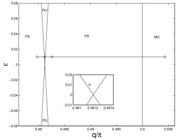
FIG. 1.: The plane of ($\epsilon,q$) where the region of the parametric instability represented by Eq. (15) is shown by two straight lines. Wavenumbers between the two “stability limits” will be (to leading order) parametrically unstable. We also highlight 4 wavenumbers for which we conduct numerical simulations, namely $q=1.50705$, $q=1.51161$, $q=1.51616$ and $q=1.58446$ , that lie on the line $\epsilon=0.01$ (see text).We use PS (PU) to indicate the parametrically stable (unstable) regions, respectively, and MU to indicate modulationally unstable ones. The vertical line $q=\pi/2$ is the boundary between the modulationally stable-unstable regions.

In the left panel of Fig. 2, we indeed observe at time $t=800$ that the perturbed wave is both parametrically and modulationally stable. On the other hand, the right panel displays $q=1.51616$, which should also be parametrically stable according to our linear theory. However, for longer times than the ones displayed in Fig. 2, the latter wavenumber has been observed to become unstable. We conjecture that this instability is due to a higher order parametric resonance, not captured within the theory of section II.

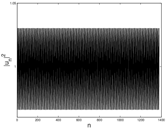
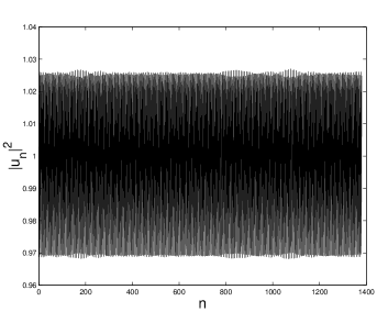
FIG. 2.: Both panels show the case where we have modulational and parametric stability. The left corresponds to $q=1.50705.$ and $t=800$ and the right to $q=1.51616$ and $t=800$. The squared amplitude ($|u|^{2}$) of the solution is shown in the panels as a function of the lattice site $n$.

The case of Fig. 3 displays the time evolution of the wavenumber predicted to be in the window of parametric instability ($q=1.511616$). We indeed find that at times $t=570$, the configuration becomes parametrically unstable.

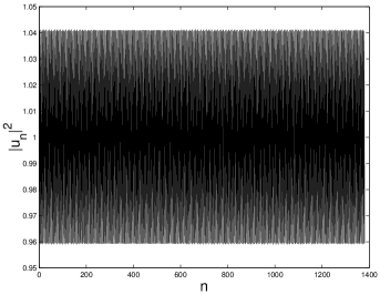
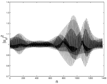
FIG. 3.: The case which is modulationally stable, but parametrically unstable. The left panel shows the square amplitude of the field before the onset of the instability at $t=570$, while the right one after it, at $t=655$. In this case $q=1.51161$.

Finally, in Fig. 4 we show the time evolution of a modulationally unstable case for $q=1.58446$. One clear feature that distinguishes the parametric instability shown in Fig. 3 from the modulational one of Fig. 4 is the time scale of the instability development, or equivalently the corresponding instability growth rate. The latter appears to be much larger in the case of the modulational instability; as a result, the MI sets in much sooner for equal magnitude perturbations of the two plane waves.

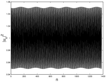
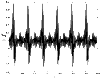
FIG. 4.: The case which is modulationally unstable. The left panel shows the square modulus of the field, before the onset of the instability at $t=17$, and right after the onset, at $t=56$. In this case $q=1.58446$.

From the growth rate predictions of Eq. $10$ of [8] and from our analysis, it can be calculated (in the cases shown) that the theoretical growth rate in the case of the modulational instability is approximately $0.23218$ (for$q=1.58446$) and the corresponding growth rate in the case of the parametric instability is approximately $0.00115$ (for $q=1.51161$). The considerably larger growth rate of the MI qualitatively justifies the earlier temporal development of the latter.

IV Conclusions

In this short communication, we have examined the potential of time-dependent coefficients, in the context of a non-autonomous discrete nonlinear Schrödinger equation, to induce a parametric instability of plane wave states. Such an instability has been identified and its boundaries established at the level of a leading order theory within a multiscale expansion. The theoretical findings have been numerically tested through direct simulations and have been found to be in agreement with the theoretical predictions (except for the regime between the parametric and modulationally unstable wavenumbers, where higher order parametric resonances may ensue).

The distinctive feature of the present parametric instability is that it has a much longer threshold time for its dynamical development in comparison with the modulational instability. This can be both quantified by means of the comparison of their respective growth rates, as well as observed in the course of direct numerical simulations. Studying the effects of parametric instabilities in other contexts including that of coherent, nonlinear wave structures in BEC is very relevant and will be addressed in future publications.

PGK gratefully acknowledges support from NSF-DMS-0204585 and from the Eppley Foundation for Research.

REFERENCES

- [1] C. Sulem and P.L. Sulem, The Nonlinear Schrödinger Equation, Springer-Verlag (New York, 1999).
- [2] T.B. Benjamin and J.E. Feir, J. Fluid. Mech. 27, 417 (1967).
- [3] L.A. Ostrovskii, Sov. Phys. JETP 24, 797 (1969).
- [4] T. Taniuti and H. Washimi, Phys. Rev. Lett. 21, 209 (1968); A. Hasegawa, Phys. Rev. Lett. 24, 1165 (1970).
- [5] M. Peyrard, T. Dauxois, H. Hoyet and C.R. Willis, Physica 68D, 104 (1993).
- [6] D. N. Christodoulides and R. I. Joseph, Opt. Lett. 13, 794 (1988)
- [7] R. Morandotti, U. Peschel, J.S. Aitchison, H.S. Eisenberg and Y. Silberberg, Phys. Rev. Lett. 83, 2726 (1999).
- [8] Yu.S. Kivshar and M. Peyrard, Phys. Rev. A 46, 3198 (1992).
- [9] B. Wu and Q. Niu, Phys. Rev. A 64, 061603(R) (2001).
- [10] A. Smerzi, A. Trombettoni, P.G. Kevrekidis and A.R. Bishop, Phys. Rev. Lett., 89, 170402 (2002).
- [11] V. V. Konotop, and M. Salerno, Phys. Rev. A65, 021602 (2002).
- [12] F. S. Cataliotti et al., New Journal of Physics 5, 71 (2003).
- [13] A. Trombettoni and A. Smerzi, Phys. Rev. Lett. 86, 2353, (2001).
- [14] F.Kh. Abdullaev, B.B. Baizakov, S.A. Darmanyan, V.V. Konotop, and M. Salerno, Phys. Rev. A64, 043606 (2001).
- [15] G.L. Alfimov, P.G. Kevrekidis, V.V. Konotop, and M. Salerno Phys. Rev. E 66, 046608 (2002)
- [16] S. Inouye et al., Nature 392, 151 (1998); J. Stenger et al., Phys. Rev. Lett. 82, 2422 (1999).
- [17] F.Kh. Abdullaev, E.N. Tsoy, B.A. Malomed, R.A. Kraenkel, cond-mat/0306281; F.Kh. Abdullaev, J.G. Caputo, R.A. Kraenkel, B.A. Malomed, cond-mat/0209219.
- [18] E.A. Donley et al., Nature 412, 295 (2001).
- [19] P.G. Kevrekidis, G. Theocharis, D.J. Frantzeskakis and B.A. Malomed, Phys. Rev. Lett. 90, 230401 (2003).
- [20] G.D. Montesinos, V.M. Perez-Garcia and P. Torres, nlin.PS/0305030.
- [21] L.D. Landau and E.M. Lifshitz, Mechanics (Pergamon, Oxford, 1973).
- [22] K. Staliunas, S. Longhi and G. J. de Valcárcel, Phys. Rev. Lett. 89, 210406 (2002).
- [23] F.Kh. Abdullaev, S.A. Darmanyan, A. Kobyakov, F. Lederer, Physics Letters A 220 (1996) 213-218.
- [24] W. Magnus and S. Winkler, Hill’s Equation (Wiley, New York, 1966).
- [25] C.M. Bender and S.A. Orszag, Advanced Mathematical Methods for Scientists and Engineers, (McGraw-Hill Publishing Company, New York 1978).