Effective Drag Between Strongly Inhomogeneous Layers: Exact Results and Applications

Abstract

We generalize Dykhne’s calculation of the effective resistance of a 2D two-component medium to the case of frictional drag between the two parallel two-component layers. The resulting exact expression for the effective transresistance, $\rho^{\mbox{$D$}}_{\mbox{eff}}$, is analyzed in the limits when the resistances and transresistances of the constituting components are strongly different - situation generic for the vicinity of the classical (percolative) metal-insulator transition (MIT). On the basis of this analysis we conclude that the evolution of $\rho^{\mbox{$D$}}_{\mbox{eff}}$ across the MIT is determined by the type of correlation between the components, constituting the 2D layers. Depending on this correlation, in the case of two electron layers, $\rho^{\mbox{$D$}}_{\mbox{eff}}$ changes either monotonically or exhibits a sharp maximum. For electron-hole layers $\rho^{\mbox{$D$}}_{\mbox{eff}}$ is negative and $\left|\rho^{\mbox{$D$}}_{\mbox{eff}}\right|$ exhibits a sharp minimum at the MIT.

Introduction. Frictional drag between two layers has been first predicted theoretically[1, 2] and later observed experimentally[3, 4]. The characteristics measured in experiment is the drag resistance, $\rho^{\mbox{$D$}}=V^{p}/I^{a}$, where, $V^{p}$, is the voltage, built up in the passive layer upon passing the current, $I^{a}$, through the active layer. Experimental observations[3, 4] have inspired a great number of theoretical studies of the frictional drag for different realizations of the 2D electron (hole) systems, constituting active and passive layers[5, 6, 7, 8, 9, 10, 11, 12, 13, 14, 15, 16, 17, 18, 19, 20]. In parallel, a general formalism for calculating of drag was advanced[21, 22, 23, 24, 25, 26, 27].

In all theoretical papers published by now, the parallel layers were assumed perfectly homogeneous on the macroscopic scales (usually, the scales exceeding the carrier mean free path, $l$). Incorporating tunneling bridges[13] or assuming correlations between the wave functions of the two layers[14] did not violate their macroscopic homogeneity. Also, except for Refs. [17, 18], the temperature was assumed high enough, thus allowing to neglect the mesoscopic fluctuations due to coherence of different regions of the layers. The question about the magnitude of drag between the 2D layers, which are strongly inhomogeneous macroscopically was not addressed in the theories[5, 6, 7, 8, 9, 10, 11, 12, 13, 14, 15, 16, 17, 18, 19, 20, 21, 22, 23, 24, 25, 26, 27]. This question is studied in the present paper.

To be specific, consider first the following situation. Assume that the passive layer is a good metal, $k_{F}l_{p}\gg 1$, which is perfectly homogeneous with a fixed concentration of electrons, $n_{p}=k_{F}^{2}/2\pi$. The concentration, $n_{a}(\mathchoice{{\hbox{\boldmath$\displaystyle r$}}}{{\hbox{\boldmath$\textstyle r$}}}{{\hbox{\boldmath$\scriptstyle r$}}}{{\hbox{\boldmath$\scriptscriptstyle r$}}})$, of electrons in the active layer is determined by the concentration of donors, $N_{D}(\mathchoice{{\hbox{\boldmath$\displaystyle r$}}}{{\hbox{\boldmath$\textstyle r$}}}{{\hbox{\boldmath$\scriptstyle r$}}}{{\hbox{\boldmath$\scriptscriptstyle r$}}})$. Due to, say, imperfections in the doping process, $N_{D}(\mathchoice{{\hbox{\boldmath$\displaystyle r$}}}{{\hbox{\boldmath$\textstyle r$}}}{{\hbox{\boldmath$\scriptstyle r$}}}{{\hbox{\boldmath$\scriptscriptstyle r$}}})$ fluctuates on a macroscopic scale with very large correlation length, $R_{c}\gg l$ (such an assumption was previously adopted in Refs.[28, 29]). Assume now, that the active layer can be depleted by applying the gate voltage, $V_{g}$. Without the gate voltage, $V_{g}=0$, we have $n_{a}(\mathchoice{{\hbox{\boldmath$\displaystyle r$}}}{{\hbox{\boldmath$\textstyle r$}}}{{\hbox{\boldmath$\scriptstyle r$}}}{{\hbox{\boldmath$\scriptscriptstyle r$}}})=N_{D}(\mathchoice{{\hbox{\boldmath$\displaystyle r$}}}{{\hbox{\boldmath$\textstyle r$}}}{{\hbox{\boldmath$\scriptstyle r$}}}{{\hbox{\boldmath$\scriptscriptstyle r$}}})$. Upon increasing $V_{g}$, the electron concentration changes as $n_{a}(\mathchoice{{\hbox{\boldmath$\displaystyle r$}}}{{\hbox{\boldmath$\textstyle r$}}}{{\hbox{\boldmath$\scriptstyle r$}}}{{\hbox{\boldmath$\scriptscriptstyle r$}}})=N_{D}(\mathchoice{{\hbox{\boldmath$\displaystyle r$}}}{{\hbox{\boldmath$\textstyle r$}}}{{\hbox{\boldmath$\scriptstyle r$}}}{{\hbox{\boldmath$\scriptscriptstyle r$}}})-\alpha V_{g}$, where the dimensionless coefficient $\alpha$ describes the depletion rate. Assume also, that at $V_{g}=0$ the concentration, $n_{a}$, is high enough, so that even with fluctuations, every region of the active layer is metallic. As $V_{g}$ increases, the local resistivities $\rho^{a}(\mathchoice{{\hbox{\boldmath$\displaystyle r$}}}{{\hbox{\boldmath$\textstyle r$}}}{{\hbox{\boldmath$\scriptstyle r$}}}{{\hbox{\boldmath$\scriptscriptstyle r$}}})=\rho^{a}\left\{N_{D}(\mathchoice{{\hbox{\boldmath$\displaystyle r$}}}{{\hbox{\boldmath$\textstyle r$}}}{{\hbox{\boldmath$\scriptstyle r$}}}{{\hbox{\boldmath$\scriptscriptstyle r$}}})-\alpha V_{g}\right\}$ will also increase, but at different rate, so that within a certain domain of $V_{g}$ the inhomogeneities in $N_{D}(\mathchoice{{\hbox{\boldmath$\displaystyle r$}}}{{\hbox{\boldmath$\textstyle r$}}}{{\hbox{\boldmath$\scriptstyle r$}}}{{\hbox{\boldmath$\scriptscriptstyle r$}}})$ will become important. Namely, while some regions of the active layer will remain metallic with $\rho^{a}=\rho^{a}_{1}$ weakly dependent on temperature, the remaining area of the active layer will turn into insulator with $\rho^{a}=\rho^{a}_{2}\propto\exp\left(\mbox{${\cal U}$}/T\right)$, where ${\cal U}$ is the activation energy. Then it is clear, that at certain critical $V_{g}=V_{g}^{c}$, the metallic regions will occupy exactly $50\%$ of the area of the active layer. In other words, the classical MIT will take place within the narrow interval $|V_{g}-V_{g}^{c}|\ll V_{g}^{c}$. The width, $\delta V_{g}$, of this interval can be related to the critical exponent, $t\approx 1.3$, of conductivity in the classical percolation[30]. Indeed, in the limit $\rho^{a}_{2}\rightarrow\infty$, the resistivity near $V_{g}^{c}$ diverges as $\rho^{a}(V_{g})\sim\rho^{a}_{1}\left[\left(V_{g}^{c}-V_{g}\right)/V_{g}^{c}\right]^{-t}$. Conversely, in the limit $\rho^{a}_{1}\rightarrow 0$, we have $\rho^{a}(V_{g})\sim\rho^{a}_{2}\left[\left(V_{g}-V_{g}^{c}\right)/V_{g}^{c}\right]^{t}$. Then $\delta V_{g}$ is determined by matching the two behaviors, i.e. $\delta V_{g}/V_{g}^{c}=\left(\rho^{a}_{1}/\rho^{a}_{2}\right)^{1/2t}$. For activated character of transport in insulator, assumed above, $\delta V_{g}$ shrinks with temperature as $\exp\left(-\mbox{${\cal U}$}/2tT\right)$.

It is important to note that, in addition to the above qualitative picture, there exists a sound quantitative result concerning resistivity at 2D classical MIT. Namely, as it was demonstrated by Dykhne[31], the exact value of $\rho^{a}$ at $V_{g}=V_{g}^{c}$ is equal to $\rho^{a}\!\left(V_{g}^{c}\right)=\left(\rho^{a}_{1}\rho^{a}_{2}\right)^{1/2}$. Moreover, the product $\rho^{a}\!\left(V_{g}^{c}+v\right)\rho^{a}\!\left(V_{g}^{c}-v\right)$ is equal to $\left(\rho^{a}_{1}\rho^{a}_{2}\right)^{1/2}$ for any $v$. Then the question arises about the behavior of the drag resistance, $\rho^{\mbox{$D$}}_{\mbox{eff}}$, in the vicinity of the classical MIT.

It is obvious that, outside the interval $|V_{g}-V_{g}^{c}|\lesssim V_{g}^{c}\left(\rho^{a}_{1}/\rho^{a}_{2}\right)^{1/2t}$ the effective transresistance is equal to $\rho^{\mbox{$D$}}_{1}$ on the “metallic” side of MIT and to $\rho^{\mbox{$D$}}_{2}$ on the “insulating” side, where $\rho^{\mbox{$D$}}_{1}$, $\rho^{\mbox{$D$}}_{2}$ are the transresistivities between the regions with resistance $\rho^{a}_{1}$ and $\rho^{a}_{2}$ of the active layer and the metal of the passive layer, respectively. This is because, outside the transition region, the transport is dominated by the current paths going exclusively through the regions of either low (metallic side) or high (insulating side) resistance. The main message of the present paper is that, similar to the value of $\rho^{a}\!\!\left(V_{g}^{c}\right)$, the exact value of $\rho^{\mbox{$D$}}\!\!\left(V_{g}^{c}\right)=\rho^{\mbox{$D$}}_{\mbox{eff}}$ can be found. In particular, in the limit $\rho^{\mbox{$D$}}_{\mbox{eff}}\ll\rho^{a}_{\mbox{eff}}$ this value is given by

$$\rho^{\mbox{$D$}}_{\mbox{eff}}=\frac{\rho^{\mbox{$D$}}_{1}\sqrt{\rho_{2}^{a}}+\rho^{\mbox{$D$}}_{2}\sqrt{\rho_{1}^{a}}}{\sqrt{\rho_{1}^{a}}+\sqrt{\rho_{2}^{a}}}.$$ (1)

To analyze the temperature dependence of $\rho^{\mbox{$D$}}_{\mbox{eff}}$ one can use for $\rho^{\mbox{$D$}}_{1}$ a conventional expression for drag between two metals. Concerning the drag resistivity, $\rho^{\mbox{$D$}}_{2}$, we have assumed that the transport in the insulating regions of the active layer is due to activated electrons. For these electrons, collisions with electrons in the passive layer, can be viewed as an additional source of scattering. From here we conclude, that both the conductance and transconductance for the insulating regions are $\propto\exp\left(-\mbox{${\cal U}$}/T\right)$. In transresistance, however, this exponent cancels out, so that the $T$-dependence of $\rho^{\mbox{$D$}}_{2}$ is weak. It is obvious from Eq. (1) that the magnitude of $\rho^{\mbox{$D$}}_{\mbox{eff}}$ lies between $\rho^{\mbox{$D$}}_{1}$ and $\rho^{\mbox{$D$}}_{2}\gg\rho^{\mbox{$D$}}_{1}$. Since $\rho_{1}^{a}\ll\rho_{2}^{a}$, Eq. (1) can be simplified to $\rho^{\mbox{$D$}}_{\mbox{eff}}=\rho^{\mbox{$D$}}_{1}+\rho^{\mbox{$D$}}_{2}\left[\rho_{1}^{a}/\rho_{2}^{a}\right]^{1/2}$, so that at low $T$ we have $\rho^{\mbox{$D$}}_{\mbox{eff}}\propto T^{2}$. With increasing $T$ this dependence crosses over to $\rho^{\mbox{$D$}}_{\mbox{eff}}\propto\exp\left(-\mbox{${\cal U}$}/2T\right)$, i.e. becomes activational. From Eq. (1) we also conclude that the effective drag does not follow the evolution of resistivity, $\rho^{a}_{\mbox{eff}}$, as the classical MIT is continuously swept, due to the variation of the gate voltage. Indeed, the $\rho^{a}_{\mbox{eff}}$ changes sharply from $\rho_{1}^{a}$ on the metallic side to $\left(\rho_{1}^{a}\rho_{2}^{a}\right)^{1/2}$ at the percolation threshold, and further to $\rho_{2}^{a}$ on the insulating side. On the other hand, the crossover of $\rho^{\mbox{$D$}}_{\mbox{eff}}$ from $\rho^{\mbox{$D$}}_{1}$ to $\rho^{\mbox{$D$}}_{2}$ is “delayed”, as illustrated in Fig. 1.

The reason why the exact expression for $\rho^{\mbox{$D$}}_{\mbox{eff}}$ can be obtained is that the duality transformation[31], which yields a closed equation for the $\rho^{a}_{\mbox{eff}}$ at MIT can be generalized to the case of two layers. This is because, the double-layer system can be viewed as a two-component system, in which each component consists of two vertically-separated islands, coupled by the mutual drag. Duality transformation between the two types of coupled islands, as depicted in Fig. 1, renders a closed matrix equation for the components of the effective resistivity matrix of the two-layer system. The corresponding steps are outlined below.

Derivation. In the presence of drag, each component of the double-layer system is characterized by its resistivity matrix

$$\mathchoice{{\hbox{\boldmath$\displaystyle{\cal R}$}}}{{\hbox{\boldmath$\textstyle{\cal R}$}}}{{\hbox{\boldmath$\scriptstyle{\cal R}$}}}{{\hbox{\boldmath$\scriptscriptstyle{\cal R}$}}}_{1}=\left(\begin{array}[]{cc}\rho_{1}^{a}&\rho^{\mbox{$D$}}_{1}\\ \rho^{\mbox{$D$}}_{1}&\rho^{p}_{1}\end{array}\right)~{}~{},~{}~{}\mathchoice{{\hbox{\boldmath$\displaystyle{\cal R}$}}}{{\hbox{\boldmath$\textstyle{\cal R}$}}}{{\hbox{\boldmath$\scriptstyle{\cal R}$}}}{{\hbox{\boldmath$\scriptscriptstyle{\cal R}$}}}_{2}=\left(\begin{array}[]{cc}\rho^{a}_{2}&\rho^{\mbox{$D$}}_{2}\\ \rho^{\mbox{$D$}}_{2}&\rho^{p}_{2}\end{array}\right).$$ (2)

If the two components are equally distributed over the plane, then the effective resistivity matrix, $\mathchoice{{\hbox{\boldmath$\displaystyle{\cal R}$}}}{{\hbox{\boldmath$\textstyle{\cal R}$}}}{{\hbox{\boldmath$\scriptstyle{\cal R}$}}}{{\hbox{\boldmath$\scriptscriptstyle{\cal R}$}}}_{\mbox{eff}}$, can be found exactly. As we demonstrate below the corresponding expression for $\mathchoice{{\hbox{\boldmath$\displaystyle{\cal R}$}}}{{\hbox{\boldmath$\textstyle{\cal R}$}}}{{\hbox{\boldmath$\scriptstyle{\cal R}$}}}{{\hbox{\boldmath$\scriptscriptstyle{\cal R}$}}}_{\mbox{eff}}$ has the form

$$\mathchoice{{\hbox{\boldmath$\displaystyle{\cal R}$}}}{{\hbox{\boldmath$\textstyle{\cal R}$}}}{{\hbox{\boldmath$\scriptstyle{\cal R}$}}}{{\hbox{\boldmath$\scriptscriptstyle{\cal R}$}}}_{\mbox{eff}} = \left(D_{1}D_{2}\right)^{1/4}\frac{D_{2}^{1/2}\mathchoice{{\hbox{\boldmath$\displaystyle{\cal R}$}}}{{\hbox{\boldmath$\textstyle{\cal R}$}}}{{\hbox{\boldmath$\scriptstyle{\cal R}$}}}{{\hbox{\boldmath$\scriptscriptstyle{\cal R}$}}}_{1}+D_{1}^{1/2}\mathchoice{{\hbox{\boldmath$\displaystyle{\cal R}$}}}{{\hbox{\boldmath$\textstyle{\cal R}$}}}{{\hbox{\boldmath$\scriptstyle{\cal R}$}}}{{\hbox{\boldmath$\scriptscriptstyle{\cal R}$}}}_{2}}{\sqrt{\det\left[D_{2}^{1/2}\mathchoice{{\hbox{\boldmath$\displaystyle{\cal R}$}}}{{\hbox{\boldmath$\textstyle{\cal R}$}}}{{\hbox{\boldmath$\scriptstyle{\cal R}$}}}{{\hbox{\boldmath$\scriptscriptstyle{\cal R}$}}}_{1}+D_{1}^{1/2}\mathchoice{{\hbox{\boldmath$\displaystyle{\cal R}$}}}{{\hbox{\boldmath$\textstyle{\cal R}$}}}{{\hbox{\boldmath$\scriptstyle{\cal R}$}}}{{\hbox{\boldmath$\scriptscriptstyle{\cal R}$}}}_{2}\right]}}$$ (3)

$$= \frac{D_{2}^{1/2}\mathchoice{{\hbox{\boldmath$\displaystyle{\cal R}$}}}{{\hbox{\boldmath$\textstyle{\cal R}$}}}{{\hbox{\boldmath$\scriptstyle{\cal R}$}}}{{\hbox{\boldmath$\scriptscriptstyle{\cal R}$}}}_{1}+D_{1}^{1/2}\mathchoice{{\hbox{\boldmath$\displaystyle{\cal R}$}}}{{\hbox{\boldmath$\textstyle{\cal R}$}}}{{\hbox{\boldmath$\scriptstyle{\cal R}$}}}{{\hbox{\boldmath$\scriptscriptstyle{\cal R}$}}}_{2}}{\sqrt{\left(D_{1}^{1/2}+D_{2}^{1/2}\right)^{2}-\det\left(\mathchoice{{\hbox{\boldmath$\displaystyle{\cal R}$}}}{{\hbox{\boldmath$\textstyle{\cal R}$}}}{{\hbox{\boldmath$\scriptstyle{\cal R}$}}}{{\hbox{\boldmath$\scriptscriptstyle{\cal R}$}}}_{1}-\mathchoice{{\hbox{\boldmath$\displaystyle{\cal R}$}}}{{\hbox{\boldmath$\textstyle{\cal R}$}}}{{\hbox{\boldmath$\scriptstyle{\cal R}$}}}{{\hbox{\boldmath$\scriptscriptstyle{\cal R}$}}}_{2}\right)}},$$ (4)

where $D_{1}=\det(\mathchoice{{\hbox{\boldmath$\displaystyle{\cal R}$}}}{{\hbox{\boldmath$\textstyle{\cal R}$}}}{{\hbox{\boldmath$\scriptstyle{\cal R}$}}}{{\hbox{\boldmath$\scriptscriptstyle{\cal R}$}}}_{1})$ and $D_{2}=\det(\mathchoice{{\hbox{\boldmath$\displaystyle{\cal R}$}}}{{\hbox{\boldmath$\textstyle{\cal R}$}}}{{\hbox{\boldmath$\scriptstyle{\cal R}$}}}{{\hbox{\boldmath$\scriptscriptstyle{\cal R}$}}}_{2})$ are the determinants of the matrices $\mathchoice{{\hbox{\boldmath$\displaystyle{\cal R}$}}}{{\hbox{\boldmath$\textstyle{\cal R}$}}}{{\hbox{\boldmath$\scriptstyle{\cal R}$}}}{{\hbox{\boldmath$\scriptscriptstyle{\cal R}$}}}_{1}$ and $\mathchoice{{\hbox{\boldmath$\displaystyle{\cal R}$}}}{{\hbox{\boldmath$\textstyle{\cal R}$}}}{{\hbox{\boldmath$\scriptstyle{\cal R}$}}}{{\hbox{\boldmath$\scriptscriptstyle{\cal R}$}}}_{2}$, respectively.

In general, the calculation of the effective resistivity requires the solution of the local Ohm equations

$$\mathchoice{{\hbox{\boldmath$\displaystyle E$}}}{{\hbox{\boldmath$\textstyle E$}}}{{\hbox{\boldmath$\scriptstyle E$}}}{{\hbox{\boldmath$\scriptscriptstyle E$}}}_{a}=\rho^{a}\mathchoice{{\hbox{\boldmath$\displaystyle J$}}}{{\hbox{\boldmath$\textstyle J$}}}{{\hbox{\boldmath$\scriptstyle J$}}}{{\hbox{\boldmath$\scriptscriptstyle J$}}}_{a}+\rho^{\mbox{$D$}}\mathchoice{{\hbox{\boldmath$\displaystyle J$}}}{{\hbox{\boldmath$\textstyle J$}}}{{\hbox{\boldmath$\scriptstyle J$}}}{{\hbox{\boldmath$\scriptscriptstyle J$}}}_{p}$$ (5)

$$\mathchoice{{\hbox{\boldmath$\displaystyle E$}}}{{\hbox{\boldmath$\textstyle E$}}}{{\hbox{\boldmath$\scriptstyle E$}}}{{\hbox{\boldmath$\scriptscriptstyle E$}}}_{p}=\rho^{p}\mathchoice{{\hbox{\boldmath$\displaystyle J$}}}{{\hbox{\boldmath$\textstyle J$}}}{{\hbox{\boldmath$\scriptstyle J$}}}{{\hbox{\boldmath$\scriptscriptstyle J$}}}_{p}+\rho^{\mbox{$D$}}\mathchoice{{\hbox{\boldmath$\displaystyle J$}}}{{\hbox{\boldmath$\textstyle J$}}}{{\hbox{\boldmath$\scriptstyle J$}}}{{\hbox{\boldmath$\scriptscriptstyle J$}}}_{a}$$ (6)

within each double-layer island constituting one of the two components, see Fig. 1. Naturally, Eqs. (5), (6) imply the in-plane isotropy of each component. Then it is convenient to view the pairs $(\mathchoice{{\hbox{\boldmath$\displaystyle J$}}}{{\hbox{\boldmath$\textstyle J$}}}{{\hbox{\boldmath$\scriptstyle J$}}}{{\hbox{\boldmath$\scriptscriptstyle J$}}}_{a},\mathchoice{{\hbox{\boldmath$\displaystyle J$}}}{{\hbox{\boldmath$\textstyle J$}}}{{\hbox{\boldmath$\scriptstyle J$}}}{{\hbox{\boldmath$\scriptscriptstyle J$}}}_{p})$ and $(\mathchoice{{\hbox{\boldmath$\displaystyle E$}}}{{\hbox{\boldmath$\textstyle E$}}}{{\hbox{\boldmath$\scriptstyle E$}}}{{\hbox{\boldmath$\scriptscriptstyle E$}}}_{a},\mathchoice{{\hbox{\boldmath$\displaystyle E$}}}{{\hbox{\boldmath$\textstyle E$}}}{{\hbox{\boldmath$\scriptstyle E$}}}{{\hbox{\boldmath$\scriptscriptstyle E$}}}_{p})$ as two-component vectors

$$\hat{\mathchoice{{\hbox{\boldmath$\displaystyle J$}}}{{\hbox{\boldmath$\textstyle J$}}}{{\hbox{\boldmath$\scriptstyle J$}}}{{\hbox{\boldmath$\scriptscriptstyle J$}}}}=\left(\begin{array}[]{c}\mathchoice{{\hbox{\boldmath$\displaystyle J$}}}{{\hbox{\boldmath$\textstyle J$}}}{{\hbox{\boldmath$\scriptstyle J$}}}{{\hbox{\boldmath$\scriptscriptstyle J$}}}_{a}\\ \mathchoice{{\hbox{\boldmath$\displaystyle J$}}}{{\hbox{\boldmath$\textstyle J$}}}{{\hbox{\boldmath$\scriptstyle J$}}}{{\hbox{\boldmath$\scriptscriptstyle J$}}}_{p}\end{array}\right)~{}~{}~{},~{}~{}~{}\hat{\mathchoice{{\hbox{\boldmath$\displaystyle E$}}}{{\hbox{\boldmath$\textstyle E$}}}{{\hbox{\boldmath$\scriptstyle E$}}}{{\hbox{\boldmath$\scriptscriptstyle E$}}}}=\left(\begin{array}[]{c}\mathchoice{{\hbox{\boldmath$\displaystyle E$}}}{{\hbox{\boldmath$\textstyle E$}}}{{\hbox{\boldmath$\scriptstyle E$}}}{{\hbox{\boldmath$\scriptscriptstyle E$}}}_{a}\\ \mathchoice{{\hbox{\boldmath$\displaystyle E$}}}{{\hbox{\boldmath$\textstyle E$}}}{{\hbox{\boldmath$\scriptstyle E$}}}{{\hbox{\boldmath$\scriptscriptstyle E$}}}_{p}\end{array}\right),$$ (7)

and rewrite local equations (5), (6) in the form

$$\hat{\mathchoice{{\hbox{\boldmath$\displaystyle E$}}}{{\hbox{\boldmath$\textstyle E$}}}{{\hbox{\boldmath$\scriptstyle E$}}}{{\hbox{\boldmath$\scriptscriptstyle E$}}}}=\mathchoice{{\hbox{\boldmath$\displaystyle{\cal R}$}}}{{\hbox{\boldmath$\textstyle{\cal R}$}}}{{\hbox{\boldmath$\scriptstyle{\cal R}$}}}{{\hbox{\boldmath$\scriptscriptstyle{\cal R}$}}}\hat{\mathchoice{{\hbox{\boldmath$\displaystyle J$}}}{{\hbox{\boldmath$\textstyle J$}}}{{\hbox{\boldmath$\scriptstyle J$}}}{{\hbox{\boldmath$\scriptscriptstyle J$}}}},$$ (8)

where the matrix, $\textstyle{\cal R}$, assumes one of the forms (2) within each component.

Local equations (8) should be solved together with Maxwell’s and continuity equations

$$\left[\mathchoice{{\hbox{\boldmath$\displaystyle\nabla$}}}{{\hbox{\boldmath$\textstyle\nabla$}}}{{\hbox{\boldmath$\scriptstyle\nabla$}}}{{\hbox{\boldmath$\scriptscriptstyle\nabla$}}}\times\hat{\mathchoice{{\hbox{\boldmath$\displaystyle E$}}}{{\hbox{\boldmath$\textstyle E$}}}{{\hbox{\boldmath$\scriptstyle E$}}}{{\hbox{\boldmath$\scriptscriptstyle E$}}}}\right]=\left(\begin{array}[]{c}\left[\mathchoice{{\hbox{\boldmath$\displaystyle\nabla$}}}{{\hbox{\boldmath$\textstyle\nabla$}}}{{\hbox{\boldmath$\scriptstyle\nabla$}}}{{\hbox{\boldmath$\scriptscriptstyle\nabla$}}}\times\mathchoice{{\hbox{\boldmath$\displaystyle E$}}}{{\hbox{\boldmath$\textstyle E$}}}{{\hbox{\boldmath$\scriptstyle E$}}}{{\hbox{\boldmath$\scriptscriptstyle E$}}}_{a}\right]\\ \left[\mathchoice{{\hbox{\boldmath$\displaystyle\nabla$}}}{{\hbox{\boldmath$\textstyle\nabla$}}}{{\hbox{\boldmath$\scriptstyle\nabla$}}}{{\hbox{\boldmath$\scriptscriptstyle\nabla$}}}\times\mathchoice{{\hbox{\boldmath$\displaystyle E$}}}{{\hbox{\boldmath$\textstyle E$}}}{{\hbox{\boldmath$\scriptstyle E$}}}{{\hbox{\boldmath$\scriptscriptstyle E$}}}_{p}\right]\end{array}\right)=0~{}~{}~{},~{}~{}~{}\left(\mathchoice{{\hbox{\boldmath$\displaystyle\nabla$}}}{{\hbox{\boldmath$\textstyle\nabla$}}}{{\hbox{\boldmath$\scriptstyle\nabla$}}}{{\hbox{\boldmath$\scriptscriptstyle\nabla$}}}\hat{\mathchoice{{\hbox{\boldmath$\displaystyle J$}}}{{\hbox{\boldmath$\textstyle J$}}}{{\hbox{\boldmath$\scriptstyle J$}}}{{\hbox{\boldmath$\scriptscriptstyle J$}}}}\right)=\left(\begin{array}[]{c}\mathchoice{{\hbox{\boldmath$\displaystyle\nabla$}}}{{\hbox{\boldmath$\textstyle\nabla$}}}{{\hbox{\boldmath$\scriptstyle\nabla$}}}{{\hbox{\boldmath$\scriptscriptstyle\nabla$}}}\mathchoice{{\hbox{\boldmath$\displaystyle J$}}}{{\hbox{\boldmath$\textstyle J$}}}{{\hbox{\boldmath$\scriptstyle J$}}}{{\hbox{\boldmath$\scriptscriptstyle J$}}}_{a}\\ \mathchoice{{\hbox{\boldmath$\displaystyle\nabla$}}}{{\hbox{\boldmath$\textstyle\nabla$}}}{{\hbox{\boldmath$\scriptstyle\nabla$}}}{{\hbox{\boldmath$\scriptscriptstyle\nabla$}}}\mathchoice{{\hbox{\boldmath$\displaystyle J$}}}{{\hbox{\boldmath$\textstyle J$}}}{{\hbox{\boldmath$\scriptstyle J$}}}{{\hbox{\boldmath$\scriptscriptstyle J$}}}_{p}\end{array}\right)=0.$$ (9)

In order to derive Eq. (4) we demonstrate that, for globally equivalent distributions of the two components, the matrix $\mathchoice{{\hbox{\boldmath$\displaystyle{\cal R}$}}}{{\hbox{\boldmath$\textstyle{\cal R}$}}}{{\hbox{\boldmath$\scriptstyle{\cal R}$}}}{{\hbox{\boldmath$\scriptscriptstyle{\cal R}$}}}_{\mbox{eff}}$ satisfies the following equation

$$\mathchoice{{\hbox{\boldmath$\displaystyle{\cal R}$}}}{{\hbox{\boldmath$\textstyle{\cal R}$}}}{{\hbox{\boldmath$\scriptstyle{\cal R}$}}}{{\hbox{\boldmath$\scriptscriptstyle{\cal R}$}}}_{\mbox{eff}}=\mathchoice{{\hbox{\boldmath$\displaystyle{\cal R}$}}}{{\hbox{\boldmath$\textstyle{\cal R}$}}}{{\hbox{\boldmath$\scriptstyle{\cal R}$}}}{{\hbox{\boldmath$\scriptscriptstyle{\cal R}$}}}_{1}\mathchoice{{\hbox{\boldmath$\displaystyle{\cal R}$}}}{{\hbox{\boldmath$\textstyle{\cal R}$}}}{{\hbox{\boldmath$\scriptstyle{\cal R}$}}}{{\hbox{\boldmath$\scriptscriptstyle{\cal R}$}}}_{\mbox{eff}}^{-1}\mathchoice{{\hbox{\boldmath$\displaystyle{\cal R}$}}}{{\hbox{\boldmath$\textstyle{\cal R}$}}}{{\hbox{\boldmath$\scriptstyle{\cal R}$}}}{{\hbox{\boldmath$\scriptscriptstyle{\cal R}$}}}_{2}.$$ (10)

This equation generalizes the Dykhne result[31] to the case of two layers coupled by drag. It is easy to see that in the absence of drag, when the matrices $\mathchoice{{\hbox{\boldmath$\displaystyle{\cal R}$}}}{{\hbox{\boldmath$\textstyle{\cal R}$}}}{{\hbox{\boldmath$\scriptstyle{\cal R}$}}}{{\hbox{\boldmath$\scriptscriptstyle{\cal R}$}}}_{1}$ and $\mathchoice{{\hbox{\boldmath$\displaystyle{\cal R}$}}}{{\hbox{\boldmath$\textstyle{\cal R}$}}}{{\hbox{\boldmath$\scriptstyle{\cal R}$}}}{{\hbox{\boldmath$\scriptscriptstyle{\cal R}$}}}_{2}$ are diagonal, Eq. (10) immediately yields the conventional expressions $\rho^{a}_{\mbox{eff}}=\sqrt{\rho^{a}_{1}\rho^{a}_{2}}$ and $\rho^{p}_{\mbox{eff}}=\sqrt{\rho^{p}_{1}\rho^{p}_{2}}$. In deriving the closed equation (10) for $\mathchoice{{\hbox{\boldmath$\displaystyle{\cal R}$}}}{{\hbox{\boldmath$\textstyle{\cal R}$}}}{{\hbox{\boldmath$\scriptstyle{\cal R}$}}}{{\hbox{\boldmath$\scriptscriptstyle{\cal R}$}}}_{\mbox{eff}}$ we follow the line of reasoning put forward by Dykhne[31]. Namely, along with $\hat{\mathchoice{{\hbox{\boldmath$\displaystyle J$}}}{{\hbox{\boldmath$\textstyle J$}}}{{\hbox{\boldmath$\scriptstyle J$}}}{{\hbox{\boldmath$\scriptscriptstyle J$}}}}$ and $\hat{\mathchoice{{\hbox{\boldmath$\displaystyle E$}}}{{\hbox{\boldmath$\textstyle E$}}}{{\hbox{\boldmath$\scriptstyle E$}}}{{\hbox{\boldmath$\scriptscriptstyle E$}}}}$, we introduce the auxiliary variables $\hat{\mathchoice{{\hbox{\boldmath$\displaystyle J$}}}{{\hbox{\boldmath$\textstyle J$}}}{{\hbox{\boldmath$\scriptstyle J$}}}{{\hbox{\boldmath$\scriptscriptstyle J$}}}}_{d}$ and $\hat{\mathchoice{{\hbox{\boldmath$\displaystyle E$}}}{{\hbox{\boldmath$\textstyle E$}}}{{\hbox{\boldmath$\scriptstyle E$}}}{{\hbox{\boldmath$\scriptscriptstyle E$}}}}_{d}$, defined as

$$\hat{\mathchoice{{\hbox{\boldmath$\displaystyle J$}}}{{\hbox{\boldmath$\textstyle J$}}}{{\hbox{\boldmath$\scriptstyle J$}}}{{\hbox{\boldmath$\scriptscriptstyle J$}}}}_{d}=\mathchoice{{\hbox{\boldmath$\displaystyle A$}}}{{\hbox{\boldmath$\textstyle A$}}}{{\hbox{\boldmath$\scriptstyle A$}}}{{\hbox{\boldmath$\scriptscriptstyle A$}}}_{J}\left[\mathchoice{{\hbox{\boldmath$\displaystyle n$}}}{{\hbox{\boldmath$\textstyle n$}}}{{\hbox{\boldmath$\scriptstyle n$}}}{{\hbox{\boldmath$\scriptscriptstyle n$}}}\times\hat{\mathchoice{{\hbox{\boldmath$\displaystyle E$}}}{{\hbox{\boldmath$\textstyle E$}}}{{\hbox{\boldmath$\scriptstyle E$}}}{{\hbox{\boldmath$\scriptscriptstyle E$}}}}\right]~{}~{}~{}~{},~{}~{}~{}~{}\hat{\mathchoice{{\hbox{\boldmath$\displaystyle E$}}}{{\hbox{\boldmath$\textstyle E$}}}{{\hbox{\boldmath$\scriptstyle E$}}}{{\hbox{\boldmath$\scriptscriptstyle E$}}}}_{d}=\mathchoice{{\hbox{\boldmath$\displaystyle A$}}}{{\hbox{\boldmath$\textstyle A$}}}{{\hbox{\boldmath$\scriptstyle A$}}}{{\hbox{\boldmath$\scriptscriptstyle A$}}}_{E}\left[\mathchoice{{\hbox{\boldmath$\displaystyle n$}}}{{\hbox{\boldmath$\textstyle n$}}}{{\hbox{\boldmath$\scriptstyle n$}}}{{\hbox{\boldmath$\scriptscriptstyle n$}}}\times\hat{\mathchoice{{\hbox{\boldmath$\displaystyle J$}}}{{\hbox{\boldmath$\textstyle J$}}}{{\hbox{\boldmath$\scriptstyle J$}}}{{\hbox{\boldmath$\scriptscriptstyle J$}}}}\right],$$ (11)

where $\mathchoice{{\hbox{\boldmath$\displaystyle A$}}}{{\hbox{\boldmath$\textstyle A$}}}{{\hbox{\boldmath$\scriptstyle A$}}}{{\hbox{\boldmath$\scriptscriptstyle A$}}}_{J}$ and $\mathchoice{{\hbox{\boldmath$\displaystyle A$}}}{{\hbox{\boldmath$\textstyle A$}}}{{\hbox{\boldmath$\scriptstyle A$}}}{{\hbox{\boldmath$\scriptscriptstyle A$}}}_{E}$ are some constant matrices, and $\textstyle n$ is the unit vector normal to the layers. It is easy to check that, similarly to $\hat{\mathchoice{{\hbox{\boldmath$\displaystyle E$}}}{{\hbox{\boldmath$\textstyle E$}}}{{\hbox{\boldmath$\scriptstyle E$}}}{{\hbox{\boldmath$\scriptscriptstyle E$}}}}$ and $\hat{\mathchoice{{\hbox{\boldmath$\displaystyle J$}}}{{\hbox{\boldmath$\textstyle J$}}}{{\hbox{\boldmath$\scriptstyle J$}}}{{\hbox{\boldmath$\scriptscriptstyle J$}}}}$, the variables, $\hat{\mathchoice{{\hbox{\boldmath$\displaystyle E$}}}{{\hbox{\boldmath$\textstyle E$}}}{{\hbox{\boldmath$\scriptstyle E$}}}{{\hbox{\boldmath$\scriptscriptstyle E$}}}}_{d}$ and $\hat{\mathchoice{{\hbox{\boldmath$\displaystyle J$}}}{{\hbox{\boldmath$\textstyle J$}}}{{\hbox{\boldmath$\scriptstyle J$}}}{{\hbox{\boldmath$\scriptscriptstyle J$}}}}_{d}$ also satisfy the Maxwell and the continuity equations

$$\left[\mathchoice{{\hbox{\boldmath$\displaystyle\nabla$}}}{{\hbox{\boldmath$\textstyle\nabla$}}}{{\hbox{\boldmath$\scriptstyle\nabla$}}}{{\hbox{\boldmath$\scriptscriptstyle\nabla$}}}\times\hat{\mathchoice{{\hbox{\boldmath$\displaystyle E$}}}{{\hbox{\boldmath$\textstyle E$}}}{{\hbox{\boldmath$\scriptstyle E$}}}{{\hbox{\boldmath$\scriptscriptstyle E$}}}}_{d}\right]=0~{}~{}~{},~{}~{}~{}\left(\mathchoice{{\hbox{\boldmath$\displaystyle\nabla$}}}{{\hbox{\boldmath$\textstyle\nabla$}}}{{\hbox{\boldmath$\scriptstyle\nabla$}}}{{\hbox{\boldmath$\scriptscriptstyle\nabla$}}}\hat{\mathchoice{{\hbox{\boldmath$\displaystyle J$}}}{{\hbox{\boldmath$\textstyle J$}}}{{\hbox{\boldmath$\scriptstyle J$}}}{{\hbox{\boldmath$\scriptscriptstyle J$}}}}_{d}\right)=0.$$ (12)

On the other hand, the Ohm’s law Eq. (8) dictates the following relation between $\hat{\mathchoice{{\hbox{\boldmath$\displaystyle E$}}}{{\hbox{\boldmath$\textstyle E$}}}{{\hbox{\boldmath$\scriptstyle E$}}}{{\hbox{\boldmath$\scriptscriptstyle E$}}}}_{d}$ and $\hat{\mathchoice{{\hbox{\boldmath$\displaystyle J$}}}{{\hbox{\boldmath$\textstyle J$}}}{{\hbox{\boldmath$\scriptstyle J$}}}{{\hbox{\boldmath$\scriptscriptstyle J$}}}}_{d}$

$$\hat{\mathchoice{{\hbox{\boldmath$\displaystyle E$}}}{{\hbox{\boldmath$\textstyle E$}}}{{\hbox{\boldmath$\scriptstyle E$}}}{{\hbox{\boldmath$\scriptscriptstyle E$}}}}_{d}=\mathchoice{{\hbox{\boldmath$\displaystyle A$}}}{{\hbox{\boldmath$\textstyle A$}}}{{\hbox{\boldmath$\scriptstyle A$}}}{{\hbox{\boldmath$\scriptscriptstyle A$}}}_{E}\left[\mathchoice{{\hbox{\boldmath$\displaystyle n$}}}{{\hbox{\boldmath$\textstyle n$}}}{{\hbox{\boldmath$\scriptstyle n$}}}{{\hbox{\boldmath$\scriptscriptstyle n$}}}\times\hat{\mathchoice{{\hbox{\boldmath$\displaystyle J$}}}{{\hbox{\boldmath$\textstyle J$}}}{{\hbox{\boldmath$\scriptstyle J$}}}{{\hbox{\boldmath$\scriptscriptstyle J$}}}}\right]=\mathchoice{{\hbox{\boldmath$\displaystyle A$}}}{{\hbox{\boldmath$\textstyle A$}}}{{\hbox{\boldmath$\scriptstyle A$}}}{{\hbox{\boldmath$\scriptscriptstyle A$}}}_{E}\left[\mathchoice{{\hbox{\boldmath$\displaystyle n$}}}{{\hbox{\boldmath$\textstyle n$}}}{{\hbox{\boldmath$\scriptstyle n$}}}{{\hbox{\boldmath$\scriptscriptstyle n$}}}\times\left(\mathchoice{{\hbox{\boldmath$\displaystyle{\cal R}$}}}{{\hbox{\boldmath$\textstyle{\cal R}$}}}{{\hbox{\boldmath$\scriptstyle{\cal R}$}}}{{\hbox{\boldmath$\scriptscriptstyle{\cal R}$}}}^{-1}\hat{\mathchoice{{\hbox{\boldmath$\displaystyle E$}}}{{\hbox{\boldmath$\textstyle E$}}}{{\hbox{\boldmath$\scriptstyle E$}}}{{\hbox{\boldmath$\scriptscriptstyle E$}}}}\right)\right]=\left(\mathchoice{{\hbox{\boldmath$\displaystyle A$}}}{{\hbox{\boldmath$\textstyle A$}}}{{\hbox{\boldmath$\scriptstyle A$}}}{{\hbox{\boldmath$\scriptscriptstyle A$}}}_{E}\mathchoice{{\hbox{\boldmath$\displaystyle{\cal R}$}}}{{\hbox{\boldmath$\textstyle{\cal R}$}}}{{\hbox{\boldmath$\scriptstyle{\cal R}$}}}{{\hbox{\boldmath$\scriptscriptstyle{\cal R}$}}}^{-1}\mathchoice{{\hbox{\boldmath$\displaystyle A$}}}{{\hbox{\boldmath$\textstyle A$}}}{{\hbox{\boldmath$\scriptstyle A$}}}{{\hbox{\boldmath$\scriptscriptstyle A$}}}_{J}^{-1}\right)\hat{\mathchoice{{\hbox{\boldmath$\displaystyle J$}}}{{\hbox{\boldmath$\textstyle J$}}}{{\hbox{\boldmath$\scriptstyle J$}}}{{\hbox{\boldmath$\scriptscriptstyle J$}}}}_{d}=\mathchoice{{\hbox{\boldmath$\displaystyle{\cal R}$}}}{{\hbox{\boldmath$\textstyle{\cal R}$}}}{{\hbox{\boldmath$\scriptstyle{\cal R}$}}}{{\hbox{\boldmath$\scriptscriptstyle{\cal R}$}}}_{d}\hat{\mathchoice{{\hbox{\boldmath$\displaystyle J$}}}{{\hbox{\boldmath$\textstyle J$}}}{{\hbox{\boldmath$\scriptstyle J$}}}{{\hbox{\boldmath$\scriptscriptstyle J$}}}}_{d}.$$ (13)

At this point we impose the duality conditions. Namely, we require that within the first component $\hat{\mathchoice{{\hbox{\boldmath$\displaystyle J$}}}{{\hbox{\boldmath$\textstyle J$}}}{{\hbox{\boldmath$\scriptstyle J$}}}{{\hbox{\boldmath$\scriptscriptstyle J$}}}}_{d}$ and $\hat{\mathchoice{{\hbox{\boldmath$\displaystyle E$}}}{{\hbox{\boldmath$\textstyle E$}}}{{\hbox{\boldmath$\scriptstyle E$}}}{{\hbox{\boldmath$\scriptscriptstyle E$}}}}_{d}$ are related via the matrix $\mathchoice{{\hbox{\boldmath$\displaystyle{\cal R}$}}}{{\hbox{\boldmath$\textstyle{\cal R}$}}}{{\hbox{\boldmath$\scriptstyle{\cal R}$}}}{{\hbox{\boldmath$\scriptscriptstyle{\cal R}$}}}_{2}$, and, conversely, within the second component the relation $\hat{\mathchoice{{\hbox{\boldmath$\displaystyle J$}}}{{\hbox{\boldmath$\textstyle J$}}}{{\hbox{\boldmath$\scriptstyle J$}}}{{\hbox{\boldmath$\scriptscriptstyle J$}}}}_{d}=\mathchoice{{\hbox{\boldmath$\displaystyle{\cal R}$}}}{{\hbox{\boldmath$\textstyle{\cal R}$}}}{{\hbox{\boldmath$\scriptstyle{\cal R}$}}}{{\hbox{\boldmath$\scriptscriptstyle{\cal R}$}}}_{1}\hat{\mathchoice{{\hbox{\boldmath$\displaystyle E$}}}{{\hbox{\boldmath$\textstyle E$}}}{{\hbox{\boldmath$\scriptstyle E$}}}{{\hbox{\boldmath$\scriptscriptstyle E$}}}}_{d}$ holds. If these conditions are met, then the equivalent distribution of the first and second components guarantees that on average $\hat{\mathchoice{{\hbox{\boldmath$\displaystyle J$}}}{{\hbox{\boldmath$\textstyle J$}}}{{\hbox{\boldmath$\scriptstyle J$}}}{{\hbox{\boldmath$\scriptscriptstyle J$}}}}_{d}$ and $\hat{\mathchoice{{\hbox{\boldmath$\displaystyle E$}}}{{\hbox{\boldmath$\textstyle E$}}}{{\hbox{\boldmath$\scriptstyle E$}}}{{\hbox{\boldmath$\scriptscriptstyle E$}}}}_{d}$ are related by the same effective resistivity matrix $\mathchoice{{\hbox{\boldmath$\displaystyle{\cal R}$}}}{{\hbox{\boldmath$\textstyle{\cal R}$}}}{{\hbox{\boldmath$\scriptstyle{\cal R}$}}}{{\hbox{\boldmath$\scriptscriptstyle{\cal R}$}}}_{\mbox{eff}}$ as the average vectors $\hat{\mathchoice{{\hbox{\boldmath$\displaystyle J$}}}{{\hbox{\boldmath$\textstyle J$}}}{{\hbox{\boldmath$\scriptstyle J$}}}{{\hbox{\boldmath$\scriptscriptstyle J$}}}}$ and $\hat{\mathchoice{{\hbox{\boldmath$\displaystyle E$}}}{{\hbox{\boldmath$\textstyle E$}}}{{\hbox{\boldmath$\scriptstyle E$}}}{{\hbox{\boldmath$\scriptscriptstyle E$}}}}$. Quantitatively, the duality conditions are expressed as

$$\mathchoice{{\hbox{\boldmath$\displaystyle{\cal R}$}}}{{\hbox{\boldmath$\textstyle{\cal R}$}}}{{\hbox{\boldmath$\scriptstyle{\cal R}$}}}{{\hbox{\boldmath$\scriptscriptstyle{\cal R}$}}}_{1}=\mathchoice{{\hbox{\boldmath$\displaystyle A$}}}{{\hbox{\boldmath$\textstyle A$}}}{{\hbox{\boldmath$\scriptstyle A$}}}{{\hbox{\boldmath$\scriptscriptstyle A$}}}_{E}\mathchoice{{\hbox{\boldmath$\displaystyle{\cal R}$}}}{{\hbox{\boldmath$\textstyle{\cal R}$}}}{{\hbox{\boldmath$\scriptstyle{\cal R}$}}}{{\hbox{\boldmath$\scriptscriptstyle{\cal R}$}}}_{2}^{-1}\mathchoice{{\hbox{\boldmath$\displaystyle A$}}}{{\hbox{\boldmath$\textstyle A$}}}{{\hbox{\boldmath$\scriptstyle A$}}}{{\hbox{\boldmath$\scriptscriptstyle A$}}}_{J}^{-1}~{}~{}~{}~{},~{}~{}~{}~{}\mathchoice{{\hbox{\boldmath$\displaystyle{\cal R}$}}}{{\hbox{\boldmath$\textstyle{\cal R}$}}}{{\hbox{\boldmath$\scriptstyle{\cal R}$}}}{{\hbox{\boldmath$\scriptscriptstyle{\cal R}$}}}_{2}=\mathchoice{{\hbox{\boldmath$\displaystyle A$}}}{{\hbox{\boldmath$\textstyle A$}}}{{\hbox{\boldmath$\scriptstyle A$}}}{{\hbox{\boldmath$\scriptscriptstyle A$}}}_{E}\mathchoice{{\hbox{\boldmath$\displaystyle{\cal R}$}}}{{\hbox{\boldmath$\textstyle{\cal R}$}}}{{\hbox{\boldmath$\scriptstyle{\cal R}$}}}{{\hbox{\boldmath$\scriptscriptstyle{\cal R}$}}}_{1}^{-1}\mathchoice{{\hbox{\boldmath$\displaystyle A$}}}{{\hbox{\boldmath$\textstyle A$}}}{{\hbox{\boldmath$\scriptstyle A$}}}{{\hbox{\boldmath$\scriptscriptstyle A$}}}_{J}^{-1}.$$ (14)

It is easy to see that these conditions are satisfied by choosing

$$\mathchoice{{\hbox{\boldmath$\displaystyle A$}}}{{\hbox{\boldmath$\textstyle A$}}}{{\hbox{\boldmath$\scriptstyle A$}}}{{\hbox{\boldmath$\scriptscriptstyle A$}}}_{E}=\mathchoice{{\hbox{\boldmath$\displaystyle{\cal R}$}}}{{\hbox{\boldmath$\textstyle{\cal R}$}}}{{\hbox{\boldmath$\scriptstyle{\cal R}$}}}{{\hbox{\boldmath$\scriptscriptstyle{\cal R}$}}}_{1}~{}~{}~{},~{}~{}~{}\mathchoice{{\hbox{\boldmath$\displaystyle A$}}}{{\hbox{\boldmath$\textstyle A$}}}{{\hbox{\boldmath$\scriptstyle A$}}}{{\hbox{\boldmath$\scriptscriptstyle A$}}}_{J}=\mathchoice{{\hbox{\boldmath$\displaystyle{\cal R}$}}}{{\hbox{\boldmath$\textstyle{\cal R}$}}}{{\hbox{\boldmath$\scriptstyle{\cal R}$}}}{{\hbox{\boldmath$\scriptscriptstyle{\cal R}$}}}_{2}^{-1}.$$ (15)

As a final step, Eq. (10) emerges from the following chain of identities for average fields and currents

$$\langle\hat{\mathchoice{{\hbox{\boldmath$\displaystyle E$}}}{{\hbox{\boldmath$\textstyle E$}}}{{\hbox{\boldmath$\scriptstyle E$}}}{{\hbox{\boldmath$\scriptscriptstyle E$}}}}_{d}\rangle=\mathchoice{{\hbox{\boldmath$\displaystyle A$}}}{{\hbox{\boldmath$\textstyle A$}}}{{\hbox{\boldmath$\scriptstyle A$}}}{{\hbox{\boldmath$\scriptscriptstyle A$}}}_{E}\left[\mathchoice{{\hbox{\boldmath$\displaystyle n$}}}{{\hbox{\boldmath$\textstyle n$}}}{{\hbox{\boldmath$\scriptstyle n$}}}{{\hbox{\boldmath$\scriptscriptstyle n$}}}\times\langle\hat{\mathchoice{{\hbox{\boldmath$\displaystyle J$}}}{{\hbox{\boldmath$\textstyle J$}}}{{\hbox{\boldmath$\scriptstyle J$}}}{{\hbox{\boldmath$\scriptscriptstyle J$}}}}\rangle\right]=\mathchoice{{\hbox{\boldmath$\displaystyle A$}}}{{\hbox{\boldmath$\textstyle A$}}}{{\hbox{\boldmath$\scriptstyle A$}}}{{\hbox{\boldmath$\scriptscriptstyle A$}}}_{E}\left[\mathchoice{{\hbox{\boldmath$\displaystyle n$}}}{{\hbox{\boldmath$\textstyle n$}}}{{\hbox{\boldmath$\scriptstyle n$}}}{{\hbox{\boldmath$\scriptscriptstyle n$}}}\times\left(\mathchoice{{\hbox{\boldmath$\displaystyle{\cal R}$}}}{{\hbox{\boldmath$\textstyle{\cal R}$}}}{{\hbox{\boldmath$\scriptstyle{\cal R}$}}}{{\hbox{\boldmath$\scriptscriptstyle{\cal R}$}}}_{\mbox{eff}}^{-1}\langle\hat{\mathchoice{{\hbox{\boldmath$\displaystyle E$}}}{{\hbox{\boldmath$\textstyle E$}}}{{\hbox{\boldmath$\scriptstyle E$}}}{{\hbox{\boldmath$\scriptscriptstyle E$}}}}\rangle\right)\right]=\left(\mathchoice{{\hbox{\boldmath$\displaystyle A$}}}{{\hbox{\boldmath$\textstyle A$}}}{{\hbox{\boldmath$\scriptstyle A$}}}{{\hbox{\boldmath$\scriptscriptstyle A$}}}_{E}\mathchoice{{\hbox{\boldmath$\displaystyle{\cal R}$}}}{{\hbox{\boldmath$\textstyle{\cal R}$}}}{{\hbox{\boldmath$\scriptstyle{\cal R}$}}}{{\hbox{\boldmath$\scriptscriptstyle{\cal R}$}}}_{\mbox{eff}}^{-1}\mathchoice{{\hbox{\boldmath$\displaystyle A$}}}{{\hbox{\boldmath$\textstyle A$}}}{{\hbox{\boldmath$\scriptstyle A$}}}{{\hbox{\boldmath$\scriptscriptstyle A$}}}_{J}^{-1}\right)\langle\hat{\mathchoice{{\hbox{\boldmath$\displaystyle J$}}}{{\hbox{\boldmath$\textstyle J$}}}{{\hbox{\boldmath$\scriptstyle J$}}}{{\hbox{\boldmath$\scriptscriptstyle J$}}}}_{d}\rangle=\mathchoice{{\hbox{\boldmath$\displaystyle{\cal R}$}}}{{\hbox{\boldmath$\textstyle{\cal R}$}}}{{\hbox{\boldmath$\scriptstyle{\cal R}$}}}{{\hbox{\boldmath$\scriptscriptstyle{\cal R}$}}}_{\mbox{eff}}~{}\!\langle\hat{\mathchoice{{\hbox{\boldmath$\displaystyle J$}}}{{\hbox{\boldmath$\textstyle J$}}}{{\hbox{\boldmath$\scriptstyle J$}}}{{\hbox{\boldmath$\scriptscriptstyle J$}}}}_{d}\rangle.$$ (16)

With $\mathchoice{{\hbox{\boldmath$\displaystyle A$}}}{{\hbox{\boldmath$\textstyle A$}}}{{\hbox{\boldmath$\scriptstyle A$}}}{{\hbox{\boldmath$\scriptscriptstyle A$}}}_{E}=\mathchoice{{\hbox{\boldmath$\displaystyle{\cal R}$}}}{{\hbox{\boldmath$\textstyle{\cal R}$}}}{{\hbox{\boldmath$\scriptstyle{\cal R}$}}}{{\hbox{\boldmath$\scriptscriptstyle{\cal R}$}}}_{1}$ and $\mathchoice{{\hbox{\boldmath$\displaystyle A$}}}{{\hbox{\boldmath$\textstyle A$}}}{{\hbox{\boldmath$\scriptstyle A$}}}{{\hbox{\boldmath$\scriptscriptstyle A$}}}_{J}^{-1}=\mathchoice{{\hbox{\boldmath$\displaystyle{\cal R}$}}}{{\hbox{\boldmath$\textstyle{\cal R}$}}}{{\hbox{\boldmath$\scriptstyle{\cal R}$}}}{{\hbox{\boldmath$\scriptscriptstyle{\cal R}$}}}_{2}$, the last identity in Eq. (16) yields Eq. (10). In general, the effective resistivity matrix is symmetric, and, thus, is characterized by three unknown elements. As a result, Eq. (10) can be reduced to three second-order algebraic equations. It turns our that only two of them are independent. More precisely, the general solution of Eq. (10) can be presented in the form

$$\mathchoice{{\hbox{\boldmath$\displaystyle{\cal R}$}}}{{\hbox{\boldmath$\textstyle{\cal R}$}}}{{\hbox{\boldmath$\scriptstyle{\cal R}$}}}{{\hbox{\boldmath$\scriptscriptstyle{\cal R}$}}}_{\mbox{eff}}=\alpha\mathchoice{{\hbox{\boldmath$\displaystyle{\cal R}$}}}{{\hbox{\boldmath$\textstyle{\cal R}$}}}{{\hbox{\boldmath$\scriptstyle{\cal R}$}}}{{\hbox{\boldmath$\scriptscriptstyle{\cal R}$}}}_{1}+\beta\mathchoice{{\hbox{\boldmath$\displaystyle{\cal R}$}}}{{\hbox{\boldmath$\textstyle{\cal R}$}}}{{\hbox{\boldmath$\scriptstyle{\cal R}$}}}{{\hbox{\boldmath$\scriptscriptstyle{\cal R}$}}}_{2},$$ (17)

where $\alpha$ and $\beta$ are the numbers. In order to find these numbers, it is sufficient to derive two relations between them. The first relation expresses the fact that the determinants of the l.h.s. and r.h.s. of Eq. (10) are equal. This yields

$$\det\left(\alpha\mathchoice{{\hbox{\boldmath$\displaystyle{\cal R}$}}}{{\hbox{\boldmath$\textstyle{\cal R}$}}}{{\hbox{\boldmath$\scriptstyle{\cal R}$}}}{{\hbox{\boldmath$\scriptscriptstyle{\cal R}$}}}_{1}+\beta\mathchoice{{\hbox{\boldmath$\displaystyle{\cal R}$}}}{{\hbox{\boldmath$\textstyle{\cal R}$}}}{{\hbox{\boldmath$\scriptstyle{\cal R}$}}}{{\hbox{\boldmath$\scriptscriptstyle{\cal R}$}}}_{2}\right)=\left(D_{1}D_{2}\right)^{1/2}.$$ (18)

The second relation emerges upon direct substitution of Eq. (17) into (10) leading to

$$\alpha^{2}\mathchoice{{\hbox{\boldmath$\displaystyle{\cal R}$}}}{{\hbox{\boldmath$\textstyle{\cal R}$}}}{{\hbox{\boldmath$\scriptstyle{\cal R}$}}}{{\hbox{\boldmath$\scriptscriptstyle{\cal R}$}}}_{1}\mathchoice{{\hbox{\boldmath$\displaystyle{\cal R}$}}}{{\hbox{\boldmath$\textstyle{\cal R}$}}}{{\hbox{\boldmath$\scriptstyle{\cal R}$}}}{{\hbox{\boldmath$\scriptscriptstyle{\cal R}$}}}_{2}^{-1}+\beta^{2}\mathchoice{{\hbox{\boldmath$\displaystyle{\cal R}$}}}{{\hbox{\boldmath$\textstyle{\cal R}$}}}{{\hbox{\boldmath$\scriptstyle{\cal R}$}}}{{\hbox{\boldmath$\scriptscriptstyle{\cal R}$}}}_{2}\mathchoice{{\hbox{\boldmath$\displaystyle{\cal R}$}}}{{\hbox{\boldmath$\textstyle{\cal R}$}}}{{\hbox{\boldmath$\scriptstyle{\cal R}$}}}{{\hbox{\boldmath$\scriptscriptstyle{\cal R}$}}}_{1}^{-1}=\left(1-2\alpha\beta\right)\mathchoice{{\hbox{\boldmath$\displaystyle{\cal I}$}}}{{\hbox{\boldmath$\textstyle{\cal I}$}}}{{\hbox{\boldmath$\scriptstyle{\cal I}$}}}{{\hbox{\boldmath$\scriptscriptstyle{\cal I}$}}},$$ (19)

where $\textstyle{\cal I}$ is the unity matrix. It follows from the above relation that nondiagonal elements of the l.h.s. are zero, so that

$$\frac{\alpha^{2}}{\beta^{2}}=\frac{\det(\mathchoice{{\hbox{\boldmath$\displaystyle{\cal R}$}}}{{\hbox{\boldmath$\textstyle{\cal R}$}}}{{\hbox{\boldmath$\scriptstyle{\cal R}$}}}{{\hbox{\boldmath$\scriptscriptstyle{\cal R}$}}}_{2})}{\det(\mathchoice{{\hbox{\boldmath$\displaystyle{\cal R}$}}}{{\hbox{\boldmath$\textstyle{\cal R}$}}}{{\hbox{\boldmath$\scriptstyle{\cal R}$}}}{{\hbox{\boldmath$\scriptscriptstyle{\cal R}$}}}_{1})}=\frac{D_{2}}{D_{1}}.$$ (20)

Upon solving the system Eqs. (18) and (20), we find the following expressions for coefficients $\alpha$ and $\beta$

$$\alpha=\frac{D_{1}^{1/4}D_{2}^{3/4}}{\sqrt{\det\left[D_{2}^{1/2}\mathchoice{{\hbox{\boldmath$\displaystyle{\cal R}$}}}{{\hbox{\boldmath$\textstyle{\cal R}$}}}{{\hbox{\boldmath$\scriptstyle{\cal R}$}}}{{\hbox{\boldmath$\scriptscriptstyle{\cal R}$}}}_{1}+D_{1}^{1/2}\mathchoice{{\hbox{\boldmath$\displaystyle{\cal R}$}}}{{\hbox{\boldmath$\textstyle{\cal R}$}}}{{\hbox{\boldmath$\scriptstyle{\cal R}$}}}{{\hbox{\boldmath$\scriptscriptstyle{\cal R}$}}}_{2}\right]}}~{}~{},~{}~{}\beta=\frac{D_{2}^{1/4}D_{1}^{3/4}}{\sqrt{\det\left[D_{2}^{1/2}\mathchoice{{\hbox{\boldmath$\displaystyle{\cal R}$}}}{{\hbox{\boldmath$\textstyle{\cal R}$}}}{{\hbox{\boldmath$\scriptstyle{\cal R}$}}}{{\hbox{\boldmath$\scriptscriptstyle{\cal R}$}}}_{1}+D_{1}^{1/2}\mathchoice{{\hbox{\boldmath$\displaystyle{\cal R}$}}}{{\hbox{\boldmath$\textstyle{\cal R}$}}}{{\hbox{\boldmath$\scriptstyle{\cal R}$}}}{{\hbox{\boldmath$\scriptscriptstyle{\cal R}$}}}_{2}\right]}}.$$ (21)

Substituting these expressions into Eq. (17), we arrive at the explicit form Eq. (4) of the effective resistivity matrix.

Applications. In all realistic situations the drag-related nondiagonal components of the matrices (2) are much smaller than the diagonal components, which describe the in-plane transport. Under this condition, the effective drag resistance between the 2D layers can be simplified to

$$\rho^{\mbox{$D$}}_{\mbox{eff}}=\frac{\rho^{\mbox{$D$}}_{1}\sqrt{\rho^{a}_{2}\rho^{p}_{2}}+\rho^{\mbox{$D$}}_{2}\sqrt{\rho^{a}_{1}\rho^{p}_{1}}}{\sqrt{\rho^{a}_{1}\rho^{p}_{2}}+\sqrt{\rho^{a}_{2}\rho^{p}_{1}}}.$$ (22)

The case of drag between a homogeneous layer and a two-component system, considered in the Introduction, corresponds to $\rho^{p}_{2}=\rho^{p}_{1}$. Then Eq. (22) immediately reduces to Eq. (1). Below we consider two more realizations of the double-layer system, in which both layers are strongly inhomogeneous.

(i) Symmetric layers. This situation (see Fig. 2) emerges when both layers are identical (e.g., positioned symmetrically with respect to the donors). Moreover, we will assume for simplicity that the gate voltages applied to the both layers are the same. Then, in the vicinity of the classical MIT, the islands (see Fig. 1) will be composed of either two metallic or two insulating components. Substituting $\rho^{p}_{1}=\rho^{a}_{1}$ and $\rho^{p}_{2}=\rho^{a}_{2}$ into Eq. (22) we obtain

$$\rho^{\mbox{$D$}}_{\mbox{eff}}=\frac{1}{2}\left[\rho^{\mbox{$D$}}_{2}\left(\frac{\rho^{a}_{1}}{\rho^{a}_{2}}\right)^{1/2}\!\!\!\!\!\!+\rho^{\mbox{$D$}}_{1}\left(\frac{\rho^{a}_{1}}{\rho^{a}_{2}}\right)^{-1/2}\right].$$ (23)

In contrast to Eq. (1), $~{}\rho^{\mbox{$D$}}_{1}$ and $\rho^{\mbox{$D$}}_{2}$ now stand for transresistances between two metals and two insulators. Similar to the case of a homogeneous passive layer, outside the MIT region we have $\rho^{\mbox{$D$}}_{\mbox{eff}}=\rho^{\mbox{$D$}}_{1}$ and $\rho^{\mbox{$D$}}_{\mbox{eff}}=\rho^{\mbox{$D$}}_{2}$, respectively. However, the behavior of $\rho^{\mbox{$D$}}_{\mbox{eff}}$ within the transition region is drastically different from that in Fig. 1. Indeed, the first term in Eq. (23) contains a small factor $\left[\rho^{a}_{1}/\rho^{a}_{2}\right]^{1/2}\propto\exp\left(-\mbox{${\cal U}$}/2T\right)$, while the second term contains a large factor $\propto\exp\left(\mbox{${\cal U}$}/2T\right)$. Thus, despite $\rho^{\mbox{$D$}}_{2}\gg\rho^{\mbox{$D$}}_{1}$, at low temperatures the second term will not only dominate, but can exceed $\rho^{\mbox{$D$}}_{2}$. As a result, $\rho^{\mbox{$D$}}_{\mbox{eff}}$ will exhibit a maximum as a function of $V_{g}$ in the vicinity of MIT, as illustrated in Fig. 2.

(ii) Electron-hole layers. The sign of transresistance in this case is negative[4]. The phenomenon of drag in the system of homogeneous electron-hole layers was previously considered in Refs. [5, 7, 8] with an emphasis on the role of interaction-induced correlations between electrons and holes beyond the random-phase approximation. We will consider the spatially inhomogeneous situation, assuming that, without disorder, the concentrations of electrons and holes are strictly equal. We will also assume that the disorder potential, acting on electrons and holes, is the same. The crucial observation is that, due to their opposite charges, electrons and holes “react” differently to the disorder potential. The same potential that creates a “metallic lake” of electrons would deplete the corresponding passive region of holes, turning them into insulator. As a result, as the MIT is approached, we arrive to the situation, depicted in Fig. 3, when the islands consist of pairs of metallic electrons and insulating holes and vice versa. Then, substituting $\rho^{\mbox{$D$}}_{2}=\rho^{\mbox{$D$}}_{1}$ , $\rho^{p}_{1}=\rho^{a}_{2}$, and $\rho^{p}_{2}=\rho^{a}_{1}$ into Eq. (22) we get

$$\rho^{\mbox{$D$}}_{\mbox{eff}}=-2\left|\rho^{\mbox{$D$}}_{1}\right|\frac{\sqrt{\rho^{a}_{1}\rho^{a}_{2}}}{\rho^{a}_{1}+\rho^{a}_{2}}.$$ (24)

It is obvious from Eq. (24) that, since $|\rho^{\mbox{$D$}}_{\mbox{eff}}|\sim\left|\rho^{\mbox{$D$}}_{1}\right|\exp\left(-\mbox{${\cal U}$}/2T\right)$, the absolute value of the effective drag exhibits a minimum near $V_{g}^{c}$, as illustrated in Fig. 3.

Discussion. In addition to the drag resistance at MIT, Eq. (4) allows to calculate the drag-induced corrections to the effective conductivity of individual layers. For the case of a homogeneous passive layer, considered in the Introduction, this correction has a form

$$\sigma_{\mbox{eff}}-\frac{1}{\sqrt{\rho^{a}_{1}\rho^{a}_{2}}}=-\frac{1}{2\rho^{p}\sqrt{\rho^{a}_{1}\rho^{a}_{2}}}\left(\frac{\rho^{\mbox{$D$}}_{1}-\rho^{\mbox{$D$}}_{2}}{\sqrt{\rho^{a}_{1}}+\sqrt{\rho^{a}_{2}}}\right)^{2}.$$ (25)

It is noteworthy, that the sign of the correction Eq. (25) is strictly negative. The reason for that is the underlying physics of the drag phenomenon. Namely, for electrons in a passive layer, their interaction with electrons in an active layer, that gives rise to drag, can be also viewed as an additional source of their scattering. Therefore at the special point $\rho^{\mbox{$D$}}_{1}=\rho^{\mbox{$D$}}_{2}$, when the r.h.s. of Eq. (25) turns to zero, it should be expected that the fourth-order correction to $\sigma_{\mbox{eff}}$, neglected in Eq. (25), has also a negative sign.

Physical explanation of the fact that $|\rho^{\mbox{$D$}}_{\mbox{eff}}|$ between the electron-hole layers has a minimum at MIT is straightforward. Indeed, when metallic lakes of electrons are located opposite to the insulating regions of holes (see Fig. 3), then, at MIT, the current paths in the active layer are perpendicular to those in the passive layer, so that the conditions for drag are unfavorable. The origin of maximum of $\rho^{\mbox{$D$}}_{\mbox{eff}}$ at MIT for two correlated electron layers, as depicted in Fig. 2, is less transparent. One can speculate that the maximum is due to the fact that, at MIT, the current paths in two layers are long, and that, due to perfect correlation, each long path in the active layer has its “counterpart” in the passive layer. Note finally, that Eq. (4) is exact and takes into account all the orders in $\rho^{\mbox{$D$}}$. Although modeling of the classical MIT with two-component mixture is crude, we believe that, due to strong difference in resistances of the components, our predictions (1), (23), and (24) for different types of behavior of $\rho^{\mbox{$D$}}_{\mbox{eff}}$ across the MIT remain valid for realistic situations.

Acknowledgements. One of the authors (M.E.R.) is grateful to the Weizmann Institute of Science for hospitality, and especially to F. von Oppen and A. Stern for highly illuminating discussions. The work was supported by the NSF under Grant No. INT-0231010.

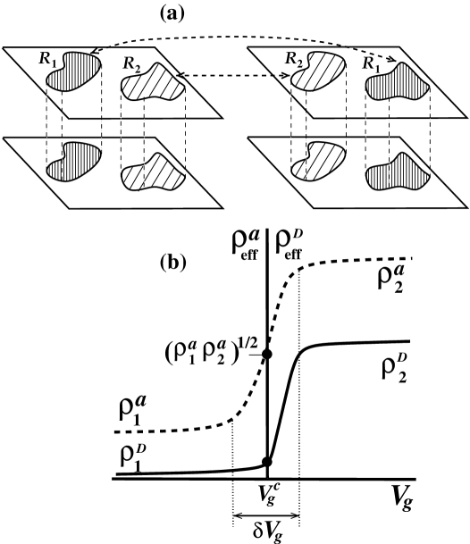
FIG. 1.: (a) Schematic illustration of the matrix duality transformation. Mutually dual two-layer islands are connected by horizontal lines; (b) The resistivity of the active layer (dashed line) and the effective drag (solid line) are depicted as a function of the gate voltage for the case when the passive layer is a homogeneous metal. The value $\rho^{\mbox{$D$}}_{\mbox{eff}}$ at MIT is given by Eq. (1), so that $\rho^{\mbox{$D$}}_{\mbox{eff}}/\rho^{\mbox{$D$}}_{2}\approx(\rho^{a}_{1}/\rho^{a}_{2})^{1/2}\ll 1$.

FIG. 2.: The transresistance across the MIT is depicted schematically for two correlated electron layers at low $T$. The value $\rho^{\mbox{$D$}}_{\mbox{eff}}$ at MIT is given by Eq. (23). The dependence $\rho^{a}_{\mbox{eff}}(V_{g})$ is the same as in Fig. 1.

FIG. 3.: The transresistance across the MIT is depicted schematically for electron-hole system. The value $\rho^{\mbox{$D$}}_{\mbox{eff}}$ at MIT is given by Eq. (24). The dependence $\rho^{a}_{\mbox{eff}}(V_{g})$ is the same as in Fig. 1.