On the Modulational Instability of the Nonlinear Schrödinger Equation with Dissipation

Abstract

The modulational instability (MI) of spatially uniform states in the nonlinear Schrödinger (NLS) equation is examined in the presence of higher-order dissipation. The study is motivated by results on the effects of three-body recombination in Bose-Einstein condensates (BECs), as well as by the important recent work of Segur et al. on the effects of linear damping in NLS settings. We show how the presence of even the weakest possible dissipation suppresses the instability on a longer time scale. However, on a shorter scale, the instability growth may take place, and a corresponding generalization of the MI criterion is developed. The analytical results are corroborated by numerical simulations. The method is valid for any power-law dissipation form, including the constant dissipation as a special case.

I Introduction

The nonlinear Schrödinger (NLS) equation is well known to be a generic model to describe evolution of envelope waves in nonlinear dispersive media. This equation applies to electromagnetic fields in optical fibers [1], deep water waves [2], Langmuir waves [3] and other types of perturbations in plasmas, such as electron-acoustic [4] waves and waves in dusty plasmas [5], macroscopic wave functions of Bose-Einstein condensates (BECs) in dilute alkali vapors [6] [in the latter case, it is usually called the Gross-Pitaevskii (GP) equation], and many other physical systems. The NLS typically appears in the Hamiltonian form

$$iu_{t}=-u_{xx}+b|u|^{2}u,$$ (1)

where $u$ is a complex envelope field and $b$ represents the strength of the nonlinearity (for instance, in the BEC context, $u$ is the mean-field wave function and $b$ is proportional to the s-wave scattering length [6]). The cases $b>0$ and $b<0$ correspond, respectively, to the self-focusing and self-defocusing NLS equation.

In many physically relevant cases, dissipation, which is ignored in Eq. (1), is not negligible. In particular, the fiber loss gives rise to a linear dissipative term in the NLS equation for optical fibers [1, 7, 8]. Dissipative phenomena have also been studied recently in the context of two-dimensional water waves [9, 10] in order to explain experimental observations in water tanks. In this setting also, the dissipation is accounted for by a linear term. In fact, it was the viewpoint of [9, 10] on the effects of damping that chiefly motivated the present work. Furthermore, it has been argued that dissipative phenomena are quite relevant in the context of BECs [11, 12]. However, in the latter case, the loss arises from higher-order processes (such as three-body recombination, corresponding to a quintic dissipation term in the GP equation [11]) or from dynamically-induced losses (such as crossing the Feshbach resonance [12, 13]). Thus, it is necessary to study models of the NLS/GP type with more complex forms of dissipative terms. Such terms were also introduced in recent studies of collapse in BECs with negative scattering length [14] and evolution of matter-wave soliton trains [15].

Higher-order loss – in the form of a term accounting for five-photon absorption – was also found to play a crucially important role (along with a cubic term that takes into regard the stimulated Raman scattering) as a mechanism arresting spatiotemporal collapse in self-focusing of light in a planar silica waveguide with the Kerr nonlinearity [16]. In this case, the high order of the absorption is explained by the fact that the ratio of the resonant absorption frequency to the carrier frequency of the photons is close to $5$.

One of the most important dynamical features of the NLS equation is the modulational instability (MI) of spatially uniform, alias continuous-wave (CW), solutions. The onset of MI leads to the formation of solitary waves and coherent structures in all of the above settings [1, 2, 3, 4, 5, 8, 9, 17, 18]. MI is a property of special interest in the above-mentioned dissipative models. In particular, as it has been recently argued [9, 10] in the context of water waves, dissipation may lead to the complete asymptotic suppression of the instability and of the formation of nonlinear waves.

The aim of the present work is to examine the MI in the context of the NLS equation with nonlinear dissipation. Motivated by the model for BECs developed in Ref. [11], but trying to keep the formulation as general as possible, we thus consider the damped NLS equation of the form:

$$iu_{t}=-u_{xx}+b|u|^{2}u+(c_{1}-ic_{2})|u|^{2k}u,$$ (2)

where $b$ and $c_{1}$ are real parameters. The constant $c_{2}$ is real and positive (in order for the corresponding term to describe loss, rather than gain). The value $k=0$ brings one back to the much studied case of the linear dissipation [1, 7, 8, 9], while $k=2$ corresponds to the quintic loss, accounting for the above-mentioned three-body recombination collision in BECs [11], and $k=5$ – to the above-mentioned case of the five-photon absorption, which is believed to be the mechanism arresting the spatiotemporal collapse in glass [16].

Our presentation is structured as follows. In Section II, we consider the MI in the general equation (2). In Section III, we focus on three special cases: (i) the (previously studied) linear damping case, (ii) $c_{2}=0$ [the Hamiltonian limit of Eq. (2)], and (iii) the case of purely dissipative nonlinearity, with $c_{1}=b=0$. In Section IV, we complement our analytical findings by numerical simulations. Section V concludes the paper.

II Modulational Instability for the Dissipative NLS Model

An exact CW (spatially uniform) solution to Eq. (2) is

$$u_{0}(t) = \left(F(t)\right)^{-1/(2k)}\exp\left[\frac{ib}{2c_{2}(1-k)}\left(F(t)\right)^{1-\frac{1}{k}}\right]$$ (3)

$$\times \exp\left[-\frac{i}{2c_{2}}\left(\frac{c_{1}}{k}\ln F(t)-\beta_{0}\right)\right],$$ (4)

where $\beta_{0}$ is an arbitrary phase shift,

$$F(t)=B_{0}^{-2k}+2kc_{2}t,$$ (5)

and $B_{0}$ is a positive constant. We now look for perturbed solutions of the NLS equation in the form

$$u(x,t)=u_{0}(t)\left[1+\epsilon w(t)\cos(qx)\right],$$ (6)

where $w(t)$ and $q$ are the amplitude and constant wavenumber of the perturbation, while $\epsilon\rightarrow 0$ is an infinitesimal perturbation parameter. Substituting (6) into (2), keeping terms linear in $\epsilon$, and splitting the perturbation amplitude in its real and imaginary parts, $w\equiv w_{r}+iw_{i}$, we obtain the following ordinary differential equations (ODEs)

$$\dot{w}_{r} = q^{2}w_{i}+2kc_{2}\left(F(t)\right)^{-1}w_{r},$$ (7)

$$\dot{w}_{i} = -\left(q^{2}+2b\left(F(t)^{-1/k}\right)+2kc_{1}\left(F(t)\right)^{-1}\right)w_{r},$$ (8)

where the overdot stands for $d/dt$. These equations can be combined into the following linear second-order equation for $w_{r}$,

$$\ddot{w}_{r}+2f(t)\dot{w}_{r}+g(t)w_{r}=0,$$ (9)

where

$$f(t) \equiv -kc_{2}/F(t),$$ (10)

$$g(t) \equiv -4k^{2}c_{2}^{2}/F(t)$$ (11)

$$+ q^{2}\left[q^{2}+2b/\left(F(t)\right)^{1/k}+2kc_{1}/F(t)\right].$$ (12)

Equation (9) can be further cast in a more standard form, $\ddot{y}+h(t)y=0,$ where $h(t)\equiv g(t)+f^{2}(t)$, and $y\equiv w_{r}(t)\exp\left(\int_{0}^{t}f(s)ds\right)$.

It follows from Eq. (12) that, in the case of the self-focusing nonlinearity ($b$, $c_{1}<0$), the initial condition $\dot{w}_{r}(0)=0$ (which we will adopt below in numerical simulations) leads to $g(0)<0$, provided that the wavenumber is chosen from the interval

$$q^{2}<q_{{\rm cr}}^{2} \equiv -(bB_{0}^{2}+kc_{1}B_{0}^{2k})$$ (13)

$$+ \sqrt{(bB_{0}^{2}+kc_{1}B_{0}^{2k})^{2}+4k^{2}c_{2}^{2}B_{0}^{4k}}.$$ (14)

The condition $g(0)<0$ implies an initial growth of the perturbation, similar to the case of MI in the usual NLS equation (1) [1, 2, 18]. It is interesting to note that, somewhat counter-intuitively, the interval (14) of unstable wavenumbers expands ($q_{{\rm cr}}^{2}$ increases) with the increase of the loss constant $c_{2}$. This result will be verified by means of numerical simulations in Sec. IV.

However, the perturbation growth can only be transient in the presence of the loss, which resembles a known situation for the MI in a conservative medium where the dispersion coefficient changes its sign in the course of the evolution (this actually pertains to evolution of an optical signal along the propagation distance in an inhomogeneous dispersive medium) [19]. In particular, even when $g(0)$ is negative (i.e., when the condition (14) is satisfied and we are in the –transiently– unstable regime), as $t$ increases, $g(t)$ increases monotonically as well and eventually becomes positive. Thus, we may expect that, until a critical time $t_{0}>0$, the function $w_{r}$ monotonically grows but then switches from growth to oscillations. This prediction also follows from the consideration of the asymptotic form of Eqs. (10) and (12) for $t\rightarrow\infty$: as the dissipation suppresses $f(t)$ and the time-dependent part of $g(t)$, in this limit Eq. (9) gives rise to oscillations of $w_{r}$ at the frequency $q^{2}$ (and, hence, to stable dynamics).

III Special cases

In this section we consider, in more detail, particular cases of special interest: (i) k=0 (ii) $c_{2}=0$, and (iii) $b=c_{1}=0$. The first case is the well-known linear damping limit (given for completeness). The second case corresponds to a higher-order version of the conservative NLS equation [see Eq. (1)], while the last one is a case of a purely dissipative nonlinearity.

A Linear Dissipation

In the limiting case $k\rightarrow 0$, Eqs. (2)-(9) lead to the following results: first, the relevant exponentially decaying solution to (2) reads

$$u_{0}(t)=\exp(-c_{2}t)\exp\left[i\left(\frac{b}{2c_{2}}\exp(-2c_{2}t)-c_{1}t+\beta_{0}\right)\right].$$ (15)

On the other hand, $w_{r}$ now satisfies the much simpler equation

$$w_{r}^{\prime\prime}+q^{2}\left[q^{2}+2b\exp(-2c_{2}t)\right]w_{r}=0,$$ (16)

which can be identified, e.g., with the equation (15.2.1) of [1] (see also [7, 8]). An explicit, though complicated, solution to this equation can be found using Bessel functions [8] and the critical time can be calculated explicitly (see e.g., [1]).

B The conservative model.

In the case $c_{2}=0$, an exact CW solution to Eq. (2) is

$$u_{0}(t)=A_{0}\exp\left[-i(bA_{0}^{2}+c_{1}A_{0}^{2k})t\right],$$ (17)

where $A_{0}$ is an arbitrary constant, and the linearized equation (9) assumes the form

$$w_{r}^{\prime\prime}+q^{2}\left[q^{2}+2(bA_{0}^{2}+kc_{1}A_{0}^{2k})\right]w_{r}=0,$$ (18)

thus giving rise to the MI criterion, $q^{2}<-2(bA_{0}^{2}+kc_{1}A_{0}^{2k})$. As it follows from here, MI is possible if either nonlinearity is self-focusing, i.e., either $b<0$ or $c_{1}<0$. If $b<0$ and the higher-order nonlinear terms are also focusing, then the interval of modulationally unstable wavenumbers grows. On the other hand, if the higher order terms are defocusing , then the corresponding interval shrinks and does so faster for higher powers (or BEC densities). In particular, the higher-order self-defocusing nonlinearity ($k>1$ and $c_{1}>0$) completely suppresses the MI if the CW amplitude is large enough, $A_{0}^{2(k-1)}>|b|/\left(kc_{1}\right)$.

C The model with dissipative nonlinearity

In the case of $b=c_{1}=0$, Eq. (9) takes a simple form,

$$w_{r}^{\prime\prime}+2\left[kc_{2}/F(t)\right]w_{r}^{\prime}+\left[q^{4}-4c_{2}^{2}k^{2}/\left(F(t)\right)^{2}\right]w_{r}=0.$$ (19)

Upon setting $\tau\equiv F(t)$, Eq. (19) reduces to

$$\tau^{2}\frac{d^{2}w_{r}}{d\tau^{2}}+\tau\frac{dw_{r}}{d\tau}+\left(\frac{q^{4}}{4c_{2}^{2}k^{2}}\tau^{2}-1\right)w_{r}=0,$$ (20)

which is the Bessel equation. Its solutions are

$$w_{r}(\tau)=A_{1}J_{1}\left(\frac{q^{2}\tau}{2c_{2}k}\right)+A_{2}Y_{1}\left(\frac{q^{2}\tau}{2c_{2}k}\right),$$ (21)

where $A_{1,2}$ are arbitrary constants, and $J_{1}$, $Y_{1}$ are the Bessel functions of the first and second kind, respectively. According to the known asymptotic properties of the Bessel functions, this solution clearly shows transition to an oscillatory behavior for large $\tau$. Notice that the case of $b=0$ and $c_{1}\neq 0$ is explicitly solvable too, through hypergeometric and Laguerre functions, but the final expressions are rather cumbersome (and hence not shown here).

IV Numerical results

The above results indicate that the linearized equation governing the evolution of the modulational perturbations can be explicitly solved only in special cases. In order to analyze the general case, we verified the long-time asymptotic predictions following from Eq. (9) by numerical simulations of this equation in the case which is most relevant to the BECs. As mentioned above, this one corresponds to $k=2$, while the other parameters in Eq. (2) are set, without loss of generality, to $b=-1$ and $c_{1}=0$ (the latter condition is adopted since, typically in the applications of interest, the conservative part of the quintic term is less significant than the dominant cubic term). Lastly, we fix $B_{0}=1$ in the CW solution (5), which is also tantamount to the general case, through a scaling transformation of Eq. (2), provided that $c_{2}$ is kept as a free parameter. Equation (9) was solved using a fourth-order Runge-Kutta integrator, with the time step $dt=0.001$, and initial conditions $w_{r}(0)=0.05$ and $\dot{w}_{r}(0)=0$.

Figure 1 illustrates the critical wavenumber bounding the MI band (of transient instability, if $c_{2}\neq 0$) as a function of the dissipation strength $c_{2}$. The solid line is the analytical prediction given by Eq. (14), which is compared with points representing numerical data. The latter were obtained by identifying the wavenumber for each value of $c_{2}$, beyond which there was no initial growth of the perturbation $w_{r}$. Good agreement is between the theoretical prediction and the numerical observations is obvious.

Figure 2 shows the difference in the evolution of modulational perturbations whose wavenumber is chosen inside (left panels) or outside (right panels) the instability band, in the absence (top panels) and in the presence (middle and bottom panels) of the quintic dissipation. The top left panel shows the case of $q=1.4$ for $c_{2}=0$, the top right illustrates the case of $q=1.5$ for the same $c_{2}$, while the middle panels demonstrate the evolution of $w_{r}$ for $|c_{2}|=0.3$, for $q=1.4$ (left panel) and $q=1.7$ (right panel). The bottom panels show the evolution of the norm in the GP equation (right panel) and the spatio-temporal evolution of a function representing the perturbation, illustrating (for $q=1$) the initial growth and eventual stabilization.

V Conclusions

In this work we studied the modulational instability (MI) in equations of the NLS type in the presence of nonlinear dissipative perturbations, motivated by the recent developments in the fields of nonlinear optics, water waves and Bose-Einstein condensates (BECs). For general power-law nonlinearities with both conservative and dissipative parts, we analyzed the spatially uniform (CW) solutions and their stability. We found that the dissipation generically suppresses the MI, switching the growth of the perturbations into an oscillatory behavior. We identified some special cases that can be analyzed exactly. Analytical predictions based on the asymptotic consideration for $t\rightarrow\infty$ were compared with numerical simulations. A noteworthy prediction (confirmed by numerical results) is that the band of wavenumbers for which the transient MI occurs expands with the increase of the strength of the dissipation.

As the MI is currently amenable to experimental observation in BECs [20], it would be particularly interesting to conduct experiments with different densities of the condensate. With a higher density, three-body recombination effects and the corresponding nonlinear dissipation are expected to be stronger, affecting the onset of the MI as predicted in this work.

PGK gratefully acknowledges support from NSF-DMS-0204585, NSF-CAREER and from the Eppley Foundation for Research. Harvey Segur is gratefully acknowledged for valuable discussions and for providing us a preprint of Ref. [9].

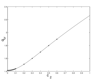
FIG. 1.: The critical wavenumber $q_{{\rm cr}}$ [see Eq. (14)] of the band which gives rise to the initial growth of modulational perturbations around the CW solution. The solid line is the analytical prediction (14), and the points show the numerical results. The parameters are $B_{0}=1$, $b=-1$, $k=2$ and $c_{1}=0$.

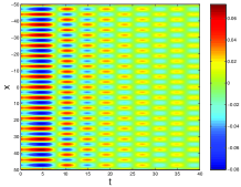
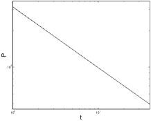
FIG. 2.: Top panels display the evolution of the modulational perturbation, $w_{r}$, in the absence of dissipation ($c_{2}=0$), for wavenumbers that do ($q=1.4$, left panel) or do not ($q=1.5$, right panel) belong to the instability band. The middle panels display the same, but in the presence of the nonlinear quintic dissipation ($|c_{2}|=0.3$), for the perturbation wavenumbers $q=1.4$ (left panel) and $q=1.7$ (right panel). The bottom panels show a typical result from the full simulation of the Gross-Pitaevskii equation for $q=1$. The left panel shows the space-time evolution of $(|u|-|u_{0}|)/|u_{0}|$, which evolves in a periodic form, whose amplitude depends on $w$. We can see in the colorbar, the initial transient growth, followed by the dissipative evolution. The right panel shows the best fit (solid line) and numerical (dashed line practically coinciding with the solid one) time evolution of the norm $P=\int|u|^{2}dx$. The best fit exponent of $\log(P)$ vs. $\log(1+1.2t)$ was found to be $-0.4994$ compared with the theoretical exponent of $-0.5$ (according to Eqs. (4)-(5)).

REFERENCES

- [1] A. Hasegawa and Y. Kodama, Solitons in optical Communications, Clarendon Press (Oxford 1995)
- [2] T. B. Benjamin and J. E. Feir, J. Fluid. Mech. 27, 417 (1967).
- [3] L. Bergé, Phys. Rep. 303, 260 (1998).
- [4] P. K. Shukla, M. A. Hellberg, and L. Stenflo, J. Atmos. Solar-Terr. Phys. 65, 355 (2003).
- [5] T. Farid, P. K. Shukla, A. M. Mirza, and L. Stenflo, Phys. Plasmas 7, 4446 (2000).
- [6] L. P. Pitaevskii and S. Stringari, Bose Einstein Condensation, Clarendon Press (Oxford, 2003); F. Dalfovo, S. Giorgini, L. P. Pitaevskii, and S. Stringari, Rev. Mod. Phys. 71, 463(1999).
- [7] D. Anderson and M. Lisak, Opt. Lett. 9, 468-470 (1984).
- [8] M. Karlsson, J. Opt. Soc. Am. B 12, 2071 (1995).
- [9] H. Segur, D. M. Henderson, J.L. Hammack, C.-M. Li, D. Pheiff and K. Socha, Stabilizing the Benjamin-Feir Instability, submitted to J. Fluid Mech. (2004).
- [10] H. Segur, Stabilizing the Benjamin-Feir Instability, Invited talk at the Fields Institute, available at: http://www.fields.utoronto.ca/audio/03-04/physics_patterns/segur/ (2003).
- [11] T. Köhler, Phys. Rev. Lett. 89, 210404 (2002).
- [12] E. A. Donley et al., Nature 412, 295 (2001). J. L. Roberts et al., Phys. Rev. Lett. 81, 5109 (1998); S. L. Cornish et al., Phys. Rev. Lett. 85, 1795 (2000);
- [13] S. Inouye et al., Nature 392, 151 (1998); J. Stenger et al., Phys. Rev. Lett. 82, 2422 (1999).
- [14] Yu. Kagan, A. E. Muryshev, and G. V. Shlyapnikov, Phys. Rev. Lett. 81, 933 (1998); H. Saito and M. Ueda, Phys. Rev. Lett. 86, 1406 (2001).
- [15] V. Y. F. Leung, A. G. Truscott, and K. G. H. Baldwin, Phys. Rev. A 66, 061602 (2002).
- [16] H. Eisenberg et al., Phys. Rev. Lett. 87, 043902 (2001).
- [17] C. Sulem and P. L. Sulem, The Nonlinear Schrödinger Equation, Springer-Verlag (New York, 1999).
- [18] A. Smerzi et al., Phys. Rev. Lett. 89, 170402; L. Salasnich, A. Parola, and L. Reatto Phys. Rev. Lett. 91, 080405 (2003); G. Theocharis et al., Phys. Rev. A 67, 063610 (2003).
- [19] B. A. Malomed, Physica Scripta 47, 311 (1993).
- [20] K. E. Strecker et al., Nature 417, 150 (2002); F. S. Cataliotti et al., New J. Phys. 5, 71 (2003).