Numerical schemes for continuum models of reaction-diffusion systems
subject to internal noise

Abstract

We present new numerical schemes to integrate stochastic partial differential equations which describe the spatio-temporal dynamics of reaction-diffusion (RD) problems under the effect of internal fluctuations. The schemes conserve the nonnegativity of the solutions and incorporate the Poissonian nature of internal fluctuations at small densities, their performance being limited by the level of approximation of density fluctuations at small scales. We apply the new schemes to two different aspects of the Reggeon model namely, the study of its non-equilibrium phase transition and the dynamics of fluctuating pulled fronts. In the latter case, our approach allows to reproduce quantitatively for the first time microscopic properties within the continuum model.

Continuum representations of the dynamics of spatially-extended systems subject to fluctuations is a very active area of research in statistical mechanics and nonlinear dynamics sancho ; barabasi ; munoz ; hohenberg ; gardiner . This is because they are frequently more tractable than discrete models, they can be put forward using simple symmetry arguments and applying conservation laws, and therefore they provide minimal representations of the observed phenomena. Important instances are Langevin equations for the relaxational dynamics of equilibrium models hohenberg , growth interface phenomena barabasi or coarse-grained descriptions of microscopic RD problems gardiner ; hinrichsen . Despite their apparent simplicity, most of these models can not be solved analytically and one has to resort to approximate analytical techniques, or to numerical integration of the stochastic time-dependent set of equations using well established algorithms kloeden . In the important instance of RD systems subject to internal fluctuations the configurations are given by a non-negative density field $\rho(x,t)$ subject to fluctuations of typical strength $\sqrt{\rho(x,t)}$ which accounts for the Poissonian fluctuations of the number of particles at $x$ gardiner . Unfortunately, standard algorithms fail to guarantee both the essential non-negativity of $\rho(x,t)$ and the Poissonian character of its fluctuations. Our purpose in this paper is to propose efficient numerical algorithms to overcome these problems which will allow us to prove the importance of internal fluctuations and to check the relevance of their correct description at different scales.

In this paper we concentrate in the so called Reggeon model, which in one dimension is given by hinrichsen

$$\frac{\partial\rho}{\partial t}=D\frac{\partial^{2}\rho}{\partial x^{2}}+\rho-\rho^{2}+\sqrt{\sigma\rho}\ \eta(x,t),$$ (1)

where $\eta(x,t)$ is a Gaussian white noise. The Reggeon model can be obtained under some approximations from the microscopic Master equations of RD microscopic models using well-known techniques gardiner ; doi . Heuristically, Eq. (1) can also be considered as the simplest dynamical equation for a coarse-grained density field with $\sigma=1/N$, $N$ being the mean-field number of particles per site. The Reggeon model provides a minimal representation of the Directed Percolation (DP) universality class, which is currently regarded as paradigm of non-equilibrium systems with absorbing states hinrichsen : if $\bar{\rho}(t)$ is the mean density spatial average, there exists a critical value of $\sigma$ for which (1) undergoes a transition between an active phase $\lim_{t\to\infty}\bar{\rho}(t)\neq 0$ and an absorbing phase for which $\lim_{t\to\infty}\bar{\rho}(t)=0$.

In addition, when $\sigma=0$ Eq. (1) becomes the so called Fisher-Kolmogorov-Petrovsky-Piscounov (FKPP) equation Fisher , which displays pulled fronts in which the active phase invades the absorbing state saarloos ; brunet ; pechenik ; doering . Simulations of microscopic particle models moro ; brunet have shown that the dynamics of pulled fronts are extremely sensitive to microscopic fluctuations at $\rho\simeq 1/N$, leading to strong corrections in the front properties when compared with those of the FKPP equation. Since Eq. (1) is usually held as a continuum description of some particle models at the mesoscopic level (i.e. when $\rho\gg 1/N$) one might doubt that the Reggeon model describes correctly the behavior of pulled fronts subject to internal fluctuations. The efficiency and accuracy of the numerical schemes proposed here will allow us to show that Eq. (1) indeed incorporates the ingredients to explain (even quantitatively) the phenomena observed in particle models, thus providing also a minimal representation of pulled fronts subject to internal fluctuations.

To simplify the discussion, let us consider the simplest possible case for the dynamics of a density subject to internal fluctuations:

$$\frac{d\rho}{dt}=a\rho+\sqrt{\sigma\rho}\>\eta(t).$$ (2)

Typical explicit or implicit methods based on stochastic Taylor approximations of (2) immediately run into problems, since they do not conserve the nonnegativity of $\rho(t)$. For example, the Euler approximation is kloeden

$$\rho_{t+\Delta t}=\rho_{t}+a\rho_{t}\Delta t+\sqrt{\sigma\rho_{t}}\Delta W_{t},$$ (3)

where $\Delta W_{t}$ are random Gaussian numbers with zero mean and $\Delta t$ variance. Thus, there is a finite probability that $\rho_{t+\Delta t}$ becomes negative, and the numerical integration comes to a halt. In order to overcome this problem, Dickman proposed an interesting solution based on the Euler scheme (3) and the discretization of the possible values of $\rho_{t}$ as multiples of $\rho^{*}={\cal O}(\sigma\Delta t)$ dickman . Despite its success in reproducing the universality class exponents of DP using (1) and its application to other situations dickman , Dickman’s algorithm is not really a numerical integration of a continuum model. Moreover, no general study of its convergence and applicability for other situations has been done yet. A more technical solution was proposed by Schurz and coworkers schurz1 using Balanced Implicit Methods (BIM), in which implicit Euler methods are used to impose the nonnegativity of the solution. In the case of Eq. (2) the BIM scheme reads note1

$$\rho_{t+\Delta t}=\frac{\rho_{t}+\Delta t\rho_{t}+\sqrt{\sigma\rho_{t}}\>(\Delta W_{t}+|\Delta W_{t}|)}{1+\sqrt{\sigma/\rho_{t}}\>|\Delta W_{t}|},$$ (4)

which explicitly implements the constraint $\rho_{t+\Delta t}\geq 0$, and reduces to the Euler algorithm (3) up to order ${\cal O}(\Delta t)$ schurz1 ; moronew . The BIM scheme is known to have the same order of convergence as the Euler algorithm, namely, the error is ${\cal O}(\sqrt{\Delta t})$ for approximations of individual trajectories and ${\cal O}(\Delta t)$ for moments of $\rho(t)$ kloeden ; schurz1 .

Another approach was taken by Pechenik and Levine pechenik employing the exact conditional probability density (CDF) ${\cal P}(\rho_{t+\Delta t}|\rho_{t})$ for the stochastic process satisfying (2), which has been known for some time in economy as the Cox-Ingersoll-Ross process cox . The CDF can be expressed in terms of modified Bessel functions and, although it can be sampled numerically using rejection or transformation methods pechenik , it is computationally expensive. Here we propose a more efficient procedure, which is based on the following: if we define $r_{d}(t)=\sum_{i=1}^{d}x_{i}^{2}(t)$, where $x_{i}(t)$ satisfies $dx_{i}/dt=ax_{i}/2+(\sigma/4)^{1/2}\eta_{i}(t)$ with $\eta_{i}(t)$ independent white noises, then $dr_{d}/dt=d\sigma/4+ar_{d}+(\sigma r_{d})^{1/2}\eta(t)$ which coincides with (2) in the limit $d\to 0$. Since the equation for each $x_{i}(t)$ is linear, $r_{d}(t)$ is the sum of squares of Gaussian random numbers with non-zero mean. Thus its probability distribution is related to the $\chi^{2}$ distribution with $d$ degrees of freedom libro . Specifically, we find that $\rho_{t+\Delta t}=r_{0}(t+\Delta t)=\chi^{\prime 2}_{0}(\lambda)/(2k)$ where $k=2a/[\sigma(e^{a\Delta t}-1)]$, $\lambda=ke^{a\Delta t}\rho_{t}$ and $\chi^{\prime 2}_{0}(\lambda)$ is a random number with a noncentral $\chi^{2}$ distribution with zero degrees of freedom and noncentrality parameter $\lambda$ whose cumulative distribution function is given by libro ; moronew ; munoznew

$${\cal P}[\chi^{2}_{0}(\lambda)\leq x]=\sum_{j=1}^{\infty}\frac{(\lambda/2)^{j}e^{-\lambda/2}}{j!}{\cal P}[\chi^{2}_{2j}\leq x]+e^{-\lambda/2}\Theta(x),$$ (5)

where $\chi^{2}_{2j}$ is a $\chi^{2}$ random number with $2j$ degrees of freedom and $\Theta(x)$ is the step function. Equation (5) is important for two reasons: (i) it shows that there is a finite probability ${\cal P}(\rho_{t+\Delta t}=0)=e^{-\lambda/2}$ for getting into the absorbing state, and more importantly (ii) it reveals that the probability distribution of $\chi^{\prime 2}_{0}(\lambda)$ is a linear combination of $\chi^{2}$ probability distributions with Poisson weights. This fact can be exploited to generate $\rho_{t+\Delta t}$ efficiently: if we choose $K$ from a Poisson distribution with mean $\lambda/2$, then

$$\rho_{t+\Delta t}=\frac{1}{2k}\left\{\begin{array}[]{ll}0&\mathrm{if}\ K=0,\\ \sum_{i=1}^{2K}z_{i}^{2}&\mathrm{if}\ K\neq 0,\end{array}\right.$$ (6)

where $z_{i}$ are independent Gaussian random numbers with zero mean and unit variance.

Figure 1: Conditional probability density as a function of $\rho_{t+\Delta t}$ for Eq. (2) with $\Delta t=0.1$, $\rho_{t}=1$ (left) and $\rho_{t}=10^{-2}$ (right). Solid lines are the exact solution from (5), while dashed lines are the approximations obtained using the Euler scheme (3).

Another interesting feature of the exact CDF for (2) is the fact that it converges asymptotically towards the Euler approximation (3) when $\lambda\simeq\rho_{t}/(\sigma\Delta t)\gg 1$ libro ; moronew . However, for small $\lambda$, the Euler approximation underestimates the large fluctuations present in the exact solution of (2). This effect, which can be seen in Fig. 1, is related to the fact that the Gaussian approximation (3) of a Poisson random number (2) is only valid when the mean value is large enough moronew . The failure of approximations like (3) or (4) to reproduce large density fluctuations at small values of $\lambda$ introduces an effective microscopic cutoff $\rho^{*}={\cal O}(\sigma\Delta t)$ in the numerical simulations below which these approximations break down.

Although the scheme (4) can be easily generalized to integrate equations like (1), this is not the case for the exact sampling of the CDF for (2). Thus, a splitting-step strategy for integrating Eq. (1) was proposed in pechenik , where the time interval $\Delta t$ is split into two steps: (i) given $\rho_{t}$, we use (6) to integrate (2) and get an intermediate value ${\tilde{\rho}}_{t+\Delta t}$; (ii) we take $\tilde{\rho}_{t+\Delta t}$ as the initial condition for $\partial\rho/\partial t=\partial^{2}\rho/\partial x^{2}-\rho^{2}$, producing $\rho_{t+\Delta t}$ with the aid of any deterministic numerical algorithm. It can be proved that this splitting step method (SSM) converges towards the solutions of (1), its order of convergence being ${\cal O}(\Delta t)$ both for realizations and for moments of $\rho(t)$ moronew . This means that the splitting-step method provides better approximations than those based on Euler methods (like the Dickman and BIM algorithms) for any realization of the noise. This has significant consequences when characterizing the critical point, as will be shown below. In the following we apply the two methods proposed here [BIM and the SSM using (6)] and the Dickman algorithm to the two problems for which Eq. (1) is archetypal .

Study of the DP phase transition. To test the proposed algorithms, we study the well known non-equilibrium phase transition that Reggeon model displays for moderate values of $\sigma$ dickman . At the critical point, the mean average density $\bar{\rho}(t)\equiv\frac{1}{L}\sum_{x}{\langle\rho(x,t)\rangle}$ decays like a power law $\bar{\rho}\sim t^{-\delta}$ with $\delta\simeq 0.1595$ hinrichsen . As in dickman , we identify the critical point as the value of $\sigma$ for which we observe such a power law decay in $\bar{\rho}(t)$. Results for the different algorithms are shown in Fig. 2, where we report the value of $\sigma_{c}$ as a function of the time step $\Delta t$. As expected, the order of convergence of the Dickman and BIM methods is ${\cal O}(\sqrt{\Delta t})$, while the SSM has ${\cal O}(\Delta t)$ order of convergence. The improvement in the order of convergence comes with a price: the computer time needed for our numerical simulations at the critical point (see table 1) indicate that methods based on Euler approximations, despite having an effective microscopic cutoff at $\rho^{*}={\cal O}(\sigma\Delta t)$, are faster than the SSM, and thus could provide better strategies for integrating numerically equations for RD models close to the critical point, where only accurate approximations of large length and time scales are needed.

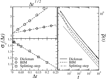
Figure 2: Left: convergence analysis for the different algorithms. Points are the critical value of $\sigma$ as a function $\Delta t$ (below) and of $\Delta t^{1/2}$ (up) while dashed lines are linear fits to the data. System size is $L=400$. Right: time dependence of the mean density $\bar{\rho}(t)$ at the critical point $\sigma=\sigma_{c}(\Delta t)$ with $\Delta t=10^{-2}$ obtained using the different algorithms (lines are shifted vertically for clarity). Thin line is the power law $\bar{\rho}(t)\sim t^{-\delta}$ with $\delta=0.1595$. System size is $L=1000$.

Table 1: Comparison of CPU time at $\sigma=\sigma_{c}(\Delta t)$ with $\Delta t=10^{-2}$ and $L=400$ for the different algorithms in Fig. 2, normalized to that of Dickman’s algorithm.

Method	$\sigma_{c}$	$T_{run}$
Dickman	2.55	1
BIM	1.61	1.2
Splitting-Step	1.45	7.6

Dynamics of fluctuating pulled fronts. When $\sigma=0$, equation (1) displays a wave-like solution (front) which travels with velocity $v_{0}=2\sqrt{D}$ (provided sharp enough initial conditions are given) Fisher ; saarloos . The dynamics of this pulled front is severely affected when microscopic fluctuations close to the absorbing state $\rho=0$ are considered. Specifically, it has been observed in particle models whose mean field limit is given by the FKPP equation, that the front speed is universally modified as brunet ; saarloos ; moro

$$v_{N}\equiv\lim_{t\to\infty}\frac{{\langle x_{f}(t)\rangle}}{t}\simeq v_{0}-v_{0}\frac{C}{\ln^{2}N},$$ (7)

where $x_{f}(t)$ is the instantaneous position of the front, $C$ is a positive constant and $N$ is the number of particles per site moro . Moreover, the pulled front diffuses with diffusion constant

$$D_{f,N}\equiv\lim_{t\to\infty}\frac{{\langle(x_{f}(t)-v_{N}t)^{2}\rangle}}{2t}\simeq\frac{C^{\prime}}{\ln^{3}N},$$ (8)

where $C^{\prime}$ is a positive constant. Whereas the velocity correction can be easily understood because microscopic fluctuations at $\rho\simeq N^{-1}$ provide an effective cutoff in the dynamics brunet , the diffusion coefficient seems to depend on the existence of relatively large fluctuations in the density at $\rho\simeq N^{-1}$ and on their slow relaxation by the pulled front dynamics moro .

As mentioned in the introduction, one might doubt that the large microscopic fluctuations at $\rho=N^{-1}$ observed in particle models are correctly reproduced by such type of equation like (1). Note, however, that the relationship between particle models and the Reggeon field model is deeper than at the coarse-grained level. Specifically, in doering it was shown that there is an exact duality transformation between the $A\leftrightarrow A+A$ microscopic particle model and the so called stochastic FKPP equation, which is similar to the Reggeon model but with a $\sqrt{\sigma\rho(1-\rho)}\>\eta(x,t)$ noise term. For $\sigma\ll 1$, the noise is only relevant at very small values of $\rho$ where $\sqrt{\sigma\rho(1-\rho)}\simeq\sqrt{\sigma\rho}$ and thus, both the Reggeon model and the stochastic FKPP should provide similar results.

Our results for the front diffusion coefficient, obtained by numerical integration of Eq. (1) are reported in Fig. 3 together with those of hybrid Monte-Carlo results for the $A\leftrightarrow A+A$ particle model moro . As we can see, for a given time step $\Delta t$, the SSM reproduces the $\ln^{-3}N$ results for particle models (8) thus confirming the duality relationship between the particle model and the continuum equation even at the quantitative level. However, the other algorithms are more consistent with a $\ln^{-6}N$ scaling which, interestingly, can be obtained through standard perturbation techniques based on Gaussian approximations for the fluctuations of the front position saarloos . The reason for this difference among the various schemes is related to the fact that both the Dickman and BIM algorithms are based on Gaussian approximations for the density fluctuations which are underestimated for $\rho<\rho^{*}={\cal O}(\sigma\Delta t)$, while only the SSM reproduces exactly the large density Poissonian fluctuations (also observed in particle models) when $\rho$ is small. This does not mean that the Dickman and BIM algorithms do not converge in this case: specifically, if we take $\Delta t\to 0$ we observe that the value of the diffusion coefficient approaches that of the hybrid MC simulations for the $A\leftrightarrow A+A$ (see Fig. 3). Thus the applicability of the Dickman and BIM algorithms is limited in this case since they fail to reproduce fluctuations at small density and time scales.

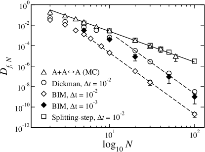
Figure 3: Front diffusion coefficient as a function of $\sigma$ for the different algorithms and different $\Delta t$, compared with hybrid MC simulations of the microscopic model $A\leftrightarrow A+A$ moro . Solid (dashed) line is the $\log^{-3}N$ ($\log^{-6}N$) power law.

In summary, we have presented new strategies for integrating stochastic (partial) differential equations for models of RD subject to internal fluctuations. While all of them preserve the nonnegativity of the solution, algorithms based on Gaussian approximations introduce a microscopic cutoff below which density fluctuations are not correctly accounted for. This is not important when the system properties are dominated by the dynamics of large length and time scales (as in critical behavior), and thus, schemes based on Euler approximation suffice to integrate numerically equations like (1). However, when the observed phenomena are sensitive to microscopic fluctuations, only algorithms which take into account the exact sampling of density fluctuations at small scales are computationally efficient. Moreover, our results validate continuum models like (1) to study the dynamics of fluctuating pulled fronts and corroborate the importance of Poissonian large fluctuations of the density at small scales. We hope that our results will be used in future for the analytical understanding of pulled front dynamics saarloos ; moro .

Finally, we mention that the methods presented here (the BIM and SSM) can be easily extended to other situations in which the relevant degrees of freedom are non-negative munoznew ; moronew , like the study of density fluctutions in more general RD problems gardiner , the understanding of critical phenomena of systems subject to external/multiplicative noise (e.g. with $\rho\>\eta(x,t)$ noises) sancho ; munoz , or the nonlinear modelling of the behavior of interest rates in economy cox ; schurz1 .

We are grateful to E. Brunet, R. Cuerno, C. Doering, H. Schurz, and P. Smereka for comments and discussions. Financial support is acknowledged from the Ministerio de Ciencia y Tecnología (Spain).

References

- (1) M. C. Cross and P. C. Hohenberg, Rev. Mod. Phys. 65, 851 (1993).
- (2) J. García-Ojalvo and J. Sancho, Noise in spatially Extended Systems (Springer-Verlag, New York, 1999).
- (3) M. A. Muñoz, in Advances in Condensed Matter and Statistical Mechanics, E. Korutcheva and R. Cuerno Eds. (Nova Sience, New York, 2004).
- (4) A.-L. Barabási and H. E. Stanley, Fractal concepts in surface growth (Cambridge Univ. Press, Cambridge, 1995); J. Krug, Adv. Phys. 46, 129 (1997).
- (5) C. W. Gardiner, Handbook of Stochastic Methods, (Springer, Berlin, 1996).
- (6) H. Hinrichsen, Adv. Phys. 49, 815 (2000).
- (7) P. E. Kloeden, E. Platen, Numerical Solution of Stochastic Differential Equations (Springer-Verlag, 1992).
- (8) M. Doi, J. Phys. A 9, 1479 (1976); L. Peliti, J. Phys. (Paris) 46, 1469 (1985); D. C. Mattis and M. L. Glasser, Rev. Mod. Phys. 70, 979 (1998).
- (9) R. A. Fisher, Ann. Eugenics VII, 355 (1936); A. Kolmogorov, I. Petrosvky, and N. Piscounov, Moscow Univ. Bull. Math. A 1, 1 (1937);
- (10) W. van Saarloos, Phys. Rep. 386 29 (2003); D. Panja, ibid, 393, 87 (2004).
- (11) E. Brunet and B. Derrida, Phys. Rev. E 56, 2597 (1997); J. Stat. Phys. 103, 269 (2001).
- (12) L. Pechenik and H. Levine, Phys. Rev. E 59, 3893 (1999).
- (13) C. R Doering, C. Mueller, and P. Smereka, Physica A 325, 243 (2003).
- (14) E. Moro, Phys. Rev. Lett. 87 238303 (2001); Phys. Rev. E 69, 060101 (2004)
- (15) While writing this paper we became aware of a recent preprint, I. Dornic, H. Chaté, M. A. Muñoz, cond-mat/0404105, in which a splitting-step like the one in pechenik and a similar procedure to compute using (5) is given.
- (16) R. Dickman, Phys. Rev. E 50, 4409 (1994); C. López and M. A. Muñoz, ibid 56, 4864 (1997).
- (17) G. N. Milshtein, E. Platen, and H. Schurz, SIAM J. Numer. Anal. 35, 1010 (1998); H. Schurz, Dyn. Syst. Appl. 5, 323 (1996).
- (18) Convergence of scheme (4) requires a cut-off at , where is chosen small enough (see schurz1 ).
- (19) E. Moro, in preparation.
- (20) J. Cox, E. Ingersoll, and S. A. Ross, Econometrics 53, 385 (1985).
- (21) N. L. Johnson, S. Kotz and N. Balakrishnan, Continuous univariate distributions (Vol. II) (John Wiley & Sons, New York, 1994); A. F. Siegel, Biometrika 66, 381 (1979).