Stochastic properties of systems controlled by autocatalytic reactions II

Abstract

We analyzed the stochastic behavior of systems controlled by autocatalytic reaction $A+X\rightleftharpoons X+X,\;\;X\rightarrow B$ provided that the distribution of reacting particles in the system volume is uniform, i.e. the point model of reaction kinetics introduced in arXiv:cond-mat/0404402 can be applied. Assuming the number of substrate particles $A$ to be kept constant by a suitable reservoir, we derived the forward Kolmogorov equation for the probability of finding $n=0,1,\ldots$ autocatalytic particles $X$ in the system at a given time moment. We have shown that the stochastic model results in an equation for the expectation value of autocatalytic particles $X$ which differs strongly from the kinetic rate equation. It has been found that not only the law of the mass action is violated but also the bifurcation point is disappeared in the well-known diagram of $X$ particle- vs. $A$ particle-concentration. Therefore, speculations about the role of autocatalytic reactions in processes of the ”natural selection” can be hardly supported.

Introduction

As in the previous paper lpal04 we define the system $\mathcal{S}$ as an aggregation of particles capable for autocatalytic reactions. Symbols $X$ and $A$ are used for notations of autocatalytic and substrate particles, respectively. We denote by $B$ the particles of end-product which do not take part in the reactions. We assume that the system is ”open” for particles $A$, i.e. the number of particles $A$ is kept constant by a suitable reservoir. However, the system is strictly closed for the autocatalytic particles $X$.

In this paper we investigate systems which are governed by reactions

$$A+{X}\stackrel{{\scriptstyle\mathrm{k_{A}}}}{{\longrightarrow}}{X}+{X},\;\;\;\;{X}+{X}\stackrel{{\scriptstyle\mathrm{k_{X}}}}{{\longrightarrow}}A+{X},\;\;\;\;{X}\stackrel{{\scriptstyle\mathrm{k_{d}}}}{{\longrightarrow}}{B},$$ (1)

where $\mathrm{k_{A}},\;\mathrm{k_{X}}$ and $\mathrm{k_{d}}$ are the rate constants. These reactions became interesting since convincing speculations were published parmon02 about the ”natural selection” based on their properties.

The organization of the paper as follows. After brief discussion of the kinetic rate equation, in Section I we derive and formally solve the forward Kolmogorov equation for the probability $p_{n}(t)$ of finding $n=0,1,\ldots\;\;X$ particles in a system of volume $V$ at time moment $t\geq 0$. Defining the conditions of the stationarity we determine the stationary probability $\lim_{t\rightarrow\infty}p_{n}(t)=w_{n}$, and analyze its properties. In Section II we present a modified stochastic model of the autocatalytic reactions (1) which is capable of reproducing the solution of the rate equation, however, brings about such a large fluctuation in the stationary number of $X$ particles, that the mean value loses practically all of its information content. In Section III we define the lifetime of a system controlled by reaction (1), and calculate exactly the extinction probability, as well as the mean value of the system lifetime. Finally, in Section IV we summarize the main conclusions.

I Stochastic model

In order to make comparison, first the well-known results of the kinetic rate equation are briefly revisited, and then the stochastic model of the reactions (1) will be thoroughly analyzed.

I.1 Rate equation

Let $m(t)$ be the number of $X$ particles in the volume $V$ of the system $\mathcal{S}$ at the time moment $t\geq 0$, and denote by $c(t)=m(t)/V$ the number-density of the $X$ particles and by $c_{A}$ that of $A$ particles which is kept strongly constant by suitable reservoir. According to the kinetic law of mass action we can write

$$\frac{dc(t)}{dt}=k_{A}c_{A}\;c(t)-k_{X}\;c^{2}(t)-k_{d}\;c(t)=k_{X}\;c(t)[c_{R}-c(t)],$$ (2)

where

$$c_{R}=\frac{k_{A}c_{A}-k_{d}}{k_{X}}$$ (3)

is the critical parameter of the reaction. Taking into account the initial condition $c(0)=c_{X}$ we obtain immediately the solution of (2) in the form:

$$c(t)=\frac{c_{X}c_{R}\exp\{c_{R}k_{X}\;t\}}{c_{R}+c_{X}(\exp\{c_{R}k_{X}\;t\}-1)},\;\;\;\;\;\;\text{if}\;c_{R}\neq 0,\;\;\;\;\;\;\text{and}\;\;\;\;\;\;c(t)=\frac{c_{X}}{1+c_{X}k_{X}\;t},\;\;\;\;\;\;\text{if}\;c_{R}=0.$$ (4)

Clearly we have two stationary solutions, namely

$$c_{st}^{(1)}=c_{R},\;\;\;\;\;\;\text{if}\;\;\;\;\;\;c_{R}>0\;\;\;\;\;\;\text{and}\;\;\;\;\;c_{st}^{(2)}=0,\;\;\;\;\;\;\text{if}\;\;\;\;\;\;c_{R}\leq 0.$$ (5)

It is easy to show that the solution of $c_{st}^{(1)}$ is stable, if $c_{A}>k_{d}/k_{A}=c_{bf}$, i.e. if $c_{R}>0$, while $c_{st}^{(2)}$ is stable, if $c_{A}\leq k_{d}/k_{A}=c_{bf}$, i.e. if $c_{R}\leq 0$. Let $\delta c$ a small disturbance in $c$. It follows from Eq. (2) that

$$\frac{d\delta c}{dt}\approx k_{X}\;[c_{R}-2c(t)]\;\delta c,$$

and so, we see immediately, if $c(t)\rightarrow c_{st}^{(1)}=c_{R}$, then $\delta c\approx\exp\{-k_{X}c_{R}t\}$, i.e. $c_{st}^{(1)}$ is stable, when $c_{R}>0$. Similarly, if $c(t)\rightarrow c_{st}^{(2)}=0$, then $\delta c\approx\exp\{k_{X}c_{R}t\}$, i.e. $c_{st}^{(2)}$ is stable, when $c_{R}<0$.

The stationary density of $X$ particles versus $c_{A}$ can be seen in FIG. 1. It is clear that $c_{A}=c_{bf}$ is a ”bifurcation point”, since if $c_{A}>c_{bf}$ then there are two stationary solutions but among them only one, namely the solution $c_{st}^{(1)}$ is stable. By decreasing the density $c_{A}$ adiabatically below the critical value $c_{bf}$, the autocatalytic particles $X$ are dying out completely, and it is impossible to start again the process by increasing the density $c_{A}$ above the critical $c_{bf}$.

FIG. 1: Dependence of the stationary number-density of $X$ particles on the number-density $c_{A}$. The thick lines refer to stable stationary values.

In the next subsection we will analyze the stochastic model of reversible reactions (1). It will be shown that in the stochastic model the long time behavior of the number of autocatalytic particles is completely different from that we obtained by using the rate equation (2).

It is to mention that interesting and seemingly convincing speculations were published parmon02 ; segre98 ; stadler93 about the possibility of ”natural selection” based on autocatalytic reactions in sets of prebiotic organic molecules and about the ”origin of life” beginning with a set of simple organic molecules capable of self-reproduction. The essence of these speculations can be summarized as follows: let us consider $\ell>1$ different and independent autocatalytic particles, and denote by $c_{bf}^{(1)}<c_{bf}^{(2)}<\cdots<c_{bf}^{(\ell)}$ the corresponding bifurcation points. If $c_{A}>c_{bf}^{(\ell)}$, then the stationary density of all autocatalytic particles is larger than zero. When the density $c_{A}$ decreases adiabatically to a value lying in the interval $(c_{bf}^{(j-1)},c_{bf}^{(j)}),\;\;j<\ell$, then the autocatalytic particles ${X}_{j},{X}_{j+1},\ldots,{X}_{\ell}$ disappear from the system, and by increasing again the density of $A$ particles above $c_{bf}^{(\ell)}$, there is no possibility to recreate those particles which were lost. In this way some form of selection can be realized. When we take into account the stochastic nature of the autocatalytic reaction, then we will see that speculations of this kind cannot be accepted.

I.2 Forward equation

Let the random function $\xi(t)$ be the number of autocatalytic particles $X$ at the time moment $t\geq 0$. The task is to determine the probability

$${\mathcal{P}}\{\xi(t)=n|\xi(0)=N_{X}\}=p_{n}(t)$$ (6)

of finding exactly $n$ autocatalytic particles $X$ in the system $\mathcal{S}$ at time instant $t\geq 0$ provided that at $t=0$ the number of ${X}$ particles was $N_{X}$. Assume that the number of the substrate particles $A$ is kept constant during the whole process, we can write for $n=1,2,\ldots$ the equation:

$$p_{n}(t+\Delta t)=p_{n}(t)\left[1-\alpha N_{A}n\;\Delta t-\frac{1}{2}\beta^{\prime}n(n-1)\;\Delta t-\gamma n\;\Delta t\right]+$$

$$+\alpha N_{A}(n-1)\;p_{n-1}(t)\;\Delta t+\left[\frac{1}{2}\beta^{\prime}n(n+1)+\gamma(n+1)\right]p_{n+1}(t)\;\Delta t+o(\Delta t),$$

and for $n=0$ the equation:

$$p_{0}(t+\Delta t)=p_{0}(t)+\gamma p_{1}(t)\;\Delta t+o(\Delta t),$$

where

$$\alpha=\frac{k_{A}}{V},\;\;\;\;\;\;\beta^{\prime}=\frac{k_{X}}{V}\;\;\;\;\;\;\text{and}\;\;\;\;\;\;\gamma=k_{d},$$ (7)

From these equations it follows immediately that

$$\frac{dp_{n}(t)}{dt}=-(\alpha N_{A}-\beta+\gamma+\beta n)\;n\;p_{n}(t)++\alpha N_{A}(n-1)\;p_{n-1}(t)+(\beta n+\gamma)(n+1)\;p_{n+1}(t),$$ (8)

$$n=1,2,\ldots,$$

where $\beta=\beta^{\prime}/2$. If $n=0$, then

$$\frac{p_{0}(t)}{dt}=\gamma p_{1}(t).$$ (9)

For the sake of completeness we derive the generating function equations

$$g(t,z)={\bf E}\{z^{\xi(t)}\}=\sum_{n=0}^{\infty}p_{n}(t)\;z^{n}$$

and

$$g_{exp}(t,y)={\bf E}\{e^{y\;\xi(t)}\}=\sum_{n=0}^{\infty}p_{n}(t)\;e^{ny}.$$

By using the equations (8) and (9) it is easy to show that $g(t,z)$ satisfies the partial differential equation

$$\frac{\partial g(t,z)}{\partial t}=-(1-z)\left(\alpha N_{A}z-\gamma\right)\;\frac{\partial g(t,z)}{\partial z}+\beta(1-z)z\;\frac{\partial^{2}g(t,z)}{\partial z^{2}},$$ (10)

while $g_{exp}(t,y)$ the equation

$$\frac{\partial g_{exp}(t,y)}{\partial t}=\left[\alpha N_{A}(e^{y}-1)+(\beta-\gamma)(1-e^{-y})\right]\;\frac{\partial g_{exp}(t,y)}{\partial y}-\beta(1-e^{-y})\;\frac{\partial^{2}g_{exp}(t,y)}{\partial y^{2}}.$$ (11)

The initial conditions are $g(0,z)=z^{N_{X}}$ and $g_{exp}(0,y)=e^{N_{X}y}$, respectively, and in addition it is to note that $g(t,1)=g_{exp}(t,0)=1$. For many purposes it is convenient to use the logarithm of the exponential generating function $g_{exp}(t,y$). Therefore, define the function

$$K(t,y)=\log\;g_{exp}(t,y)$$ (12)

the derivatives of which at $y=0$, i.e.

$$\left[\frac{\partial^{j}K(t,y)}{\partial y^{j}}\right]_{y=0}=\kappa_{j}(t),\;\;\;\;\;\;j=1,2,\ldots$$

are the cumulants of $\xi(t)$. One can immediately obtain the equation

$$\frac{\partial K(t,y)}{\partial t}=\left[\alpha N_{A}(e^{y}-1)+(\beta-\gamma)(1-e^{-y})\right]\;\frac{\partial K(t,y)}{\partial y}-\beta(1-e^{-y})\;\left\{\frac{\partial^{2}K(t,y)}{\partial y^{2}}+\left[\frac{\partial K(t,y)}{\partial y}\right]^{2}\right\}.$$ (13)

Now, the initial condition is

$$K(0,y)=N_{X}\;y,\;\;\;\;\;\;\text{while}\;\;\;\;\;\;K(t,0)=0.$$

In order to simplify the notations define the vector

$$\vec{\bf p}(t)=\left(\begin{array}[]{c}p_{0}(t)\\ p_{1}(t)\\ \vdots\\ p_{n}(t)\\ \vdots\end{array}\right)$$ (14)

and the matrix

$$\mathbf{A}=\begin{pmatrix}-D_{0}&C_{0}&0&0&0&\cdots\\ B_{1}&-D_{1}&C_{1}&0&0&\cdots\\ 0&B_{2}&-D_{2}&C_{2}&0&\cdots\\ 0&0&B_{3}&-D_{3}&C_{3}&\cdots\\ \vdots&\vdots&\vdots&\vdots&\vdots&\ddots&\end{pmatrix},$$ (15)

where

$$B_{n} = a\;(n-1),\;\;\;\;\;\;a=\frac{\alpha N_{A}}{\beta},$$ (16)

$$D_{n} = n\;(n-1+a+b),\;\;\;\;\;\;b=\frac{\gamma}{\beta},$$ (17)

$$C_{n} = (n+1)\;(n+b),$$ (18)

and write the Eqs. (8) and (9) in the following concise form:

$$\frac{d\vec{\mathbf{p}}(u)}{du}=\mathbf{A}\;\vec{\mathbf{p}}(u),\;\;\;\;\;\;\text{where}\;\;\;\;\;\;u=\beta\;t.$$ (19)

The formal solution of this equation is

$$\vec{\mathbf{p}}(u)=\exp\{\mathbf{A}u\}\;\vec{\mathbf{p}}(0),$$ (20)

where the components of $\vec{\mathbf{p}}(0)$ are $p_{n}(0)=\delta_{n,N_{X}},\;\;n=0,1,\ldots,$ and the matrix $\mathbf{A}$ is a normal Jacobi matrix. As known, the eigenvalues of a normal Jacobi matrix are different and real. If

$$\nu_{0}>\nu_{1}>\cdots>\nu_{k}>\cdots$$

are the eigenvalues of $\mathbf{A}$, then the $n$’th component of the vector $\vec{\mathbf{p}}(u)$ can be written in the form

$$p_{n}(u)=\sum_{k=0}^{\infty}w_{nk}\;e^{\nu_{k}u},$$ (21)

for any ${n\geq 0}$. Since to find the eigenvalues $\nu_{k},\;k=0,1,\ldots$ and the coefficients $w_{nk},\;n,k=0,1,\ldots$ is not a simple task, we concentrate our efforts only on the determination of stationary solutions of Eqs. (8) and (9).

I.2.1 Stationary probabilities

In order to show that the limit relations

$$\lim_{u\rightarrow\infty}p_{n}(u)=w_{n},\;\;\;\;\;\;\forall n\geq 0,\;\;n\in{\mathcal{Z}}_{+}$$ (22)

exist, we need a theorem for eigenvalues of the matrix $\mathbf{A}$ stating that $\nu_{0}=0$ and $\nu_{k}<0$ for every $k\geq 1$. The proof of the theorem can be found in Appendix A. By using this theorem it follows from Eq. (21) that

$$\lim_{u\rightarrow\infty}p_{n}(u)=w_{n0},\;\;\;\;\;\;\text{i.e.}\;\;\;\;\;\;w_{n}=w_{n0},\;\;\;\;\;\;\forall n\geq 0.$$ (23)

Since in this case

$$\lim_{u\rightarrow\infty}\frac{dp_{n}(u)}{du}=0,\;\;\;\;\;\;\forall\;n\geq 0,$$

we can write from (8) immediately the stationary equations

$$a\;[nw_{n}-(n-1)w_{n-1}]=n[(n+1)w_{n+1}-(n-1)w_{n}]+b\;[(n+1)w_{n+1}-nw_{n}],$$ (24)

for all $n\geq 1$. Summing up both sides of (24) from $n=1$ to $n=k$, we obtain

$$a\;kw_{k}=k(k+1)w_{k+1}+b\;(k+1)w_{k+1}-b\;w_{1}.$$ (25)

Taking into account the Eq. (9) we should write that

$$p_{0}(u)=b\;\int_{0}^{u}p_{1}(u^{\prime})\;du^{\prime}=b\;\left[w_{1}\;u+\sum_{k=1}^{\infty}w_{1k}\;\frac{1-e^{-|\nu_{k}|u}}{|\nu_{k}|}\right]=w_{0}+\sum_{k=1}^{\infty}w_{0k}\;e^{-|\nu_{k}|u},$$ (26)

and we see that the condition of the stationarity is either $w_{1}=0$, or $b=0$, i.e. $\gamma=0$.

If $w_{1}=0$, then it follows from (25) that $w_{n}=0$ for all $n=2,3,\ldots$, and consequently,

$$w_{0}=\gamma\;\sum_{k=1}^{\infty}\frac{w_{1k}}{|\nu_{k}|}.$$

Since

$$\sum_{n=0}^{\infty}w_{n}=w_{0}=1,\;\;\;\;\;\;\text{obviously}\;\;\;\;\;\;\gamma\;\sum_{k=1}^{\infty}\frac{w_{1k}}{|\nu_{k}|}=1.$$

If $b=\gamma/\beta=0$, i.e. if the autocatalytic particles $X$ do not decay, then $w_{0}=0$ and from (25) one obtains that

$$w_{k+1}=\frac{a}{k+1}\;w_{k},\;\;\;\;\;\;\text{i.e.}\;\;\;\;\;\;w_{n}=\frac{a^{n-1}}{n!}\;w_{1}.$$

Taking into account that $\sum_{n=1}^{\infty}w_{n}=1$ we can write

$$w_{n}=0,\;\;\;\;\;\;\text{if}\;\;\;\;\;\;\gamma\neq 0\;\;\;\;\;\;\text{and}\;\;\;\;\;\;w_{n}=\frac{a^{n}}{n!}\;\frac{e^{-a}}{1-e^{-a}},\;\;\;\;\;\;\text{if}\;\;\;\;\;\;\gamma=0,$$ (27)

for $n=1,2,\ldots$, while for $n=0$ we have

$$w_{0}=\left\{\begin{array}[]{ll}1,&\text{if $\gamma\neq 0$,}\\ \text{ }&\text{ }\\ 0,&\text{if $\gamma=0$.}\end{array}\right.$$ (28)

For the calculation of factorial moments let us introduce the generating function

$$g_{st}(z)=1,\;\;\;\;\;\;\text{if}\;\;\;\;\;\;\gamma\neq 0\;\;\;\;\;\;\text{and}\;\;\;\;\;\;g_{st}(z)=\frac{e^{-a(1-z)}-e^{-a}}{1-e^{-a}},\;\;\;\;\;\;\text{if}\;\;\;\;\;\;\gamma=0.$$ (29)

I.2.2 Expectation value and variance

In order to obtain the equation for the mean value of the number of $X$ particles we use the generating function equation (11). Introducing the time parameter $u=\beta t$ we have

$$\frac{dm_{1}(u)}{du}=m_{1}(u)[a-b+1-m_{1}(u)]-\beta\;[m_{2}(u)-m_{1}^{2}(u)],$$

which clearly shows that the kinetic law of the mass action is violated, when the variance $V(u)=m_{2}(u)-m_{1}^{2}(u)$ is not negligible. For the second moment we get the equation

$$\frac{dm_{2}(u)}{du}=(a+b-1)\;m_{1}(u)+[2(a-b)+3]\;m_{2}(u)-2\;m_{3}(u),$$

in which appears the third moment $m_{3}(u)$. There are several methods to find approximate solution of $m_{1}(t)$, some of them were mentioned already in lpal04 . Here, we do not want to discuss the details, instead we are focussing our attention on the properties of the expectation value and variance in stationary state.

If the decay constant $\gamma$ of $X$ particles is zero, then it is easy to show from Eq. (29) that the stationary value of the average number of autocatalytic particles in the system is equal to

$$m_{1}^{(st)}=\frac{a}{1-e^{-a}},$$ (30)

while the second factorial moment is

$$m_{st}^{(2)}=\frac{a^{2}}{1-e^{-a}}=a\;m_{1}^{(st)},$$ (31)

consequently, the variance can be written in the form

$$V_{st}=m_{st}^{(2)}+m_{1}^{(st)}[1-m_{1}^{(st)}]=m_{1}^{(st)}\left(1-\frac{a}{e^{a}-1}\right).$$ (32)

If $\gamma\neq 0$, then $m_{st}^{(k)}=m_{k}^{(st)}=0,\;\forall k\geq 1$.

The first important conclusion drawn from the stochastic model is that the average number of the autocatalytic particles in stationary state is different from zero, only when the decay rate constant $\gamma$ of $X$ particles is zero. It means that there is no ”bifurcation” point in the dependence of the average stationary number of $X$ particles on the number of $A$ particles, therefore speculations mentioned earlier about the ”natural selection” are not supported by the stochastic model.

The second conclusion is connected with the law of the mass action referring to the chemical equilibrium. If $\gamma=0$, then the reversible reaction $A+X\rightleftharpoons X+X$ has to lead to an equilibrium state, in which

$$m_{1}^{(st)}=N_{A}\;\frac{k_{A}}{k_{X}}=N_{A}\;\frac{\alpha}{2\;\beta}=\frac{1}{2}\;a.$$ (33)

The stochastic model results in an entirely different expression, namely

$$m_{1}^{(st)}=\frac{a}{1-e^{-a}}.$$ (34)

The relative dispersion, i.e.

$$\frac{V_{st}}{m_{1}^{(st)}}=1-\frac{a}{e^{a}-1}$$

clearly shows that the fluctuations of the number of autocatalytic particles become Poisson-like when the number of substrate particles is increasing.

II Modified stochastic model

The modification of the stochastic model is very simple. We assume that the probability of the reverse reaction $X+X\longrightarrow A+X$ is proportional to the average number of $X$ particles. Therefore, the probability that a reverse reaction occurs in the time interval $(t,t+\Delta t)$ is nothing else than $\beta\;m_{1}(t)\;n\;\Delta t+o(\Delta t)$ provided that the number of $X$ particles was exactly $n$ at time moment $t$. Accepting this assumption we can rewrite  the equations (8) and (9) in the form:

$$\frac{d\tilde{p}_{n}(t)}{dt}=-[\alpha N_{A}+\gamma+\beta m_{1}(t)]\;n\;\tilde{p}_{n}(t)+\alpha N_{A}(n-1)\;\tilde{p}_{n-1}(t)+$$

$$+[\gamma+\beta m_{1}(t)](n+1)\;\tilde{p}_{n+1}(t),\;\;\;\;\;\;n=1,2,\ldots,$$ (35)

and

$$\frac{\tilde{p}_{0}(t)}{dt}=\gamma\tilde{p}_{1}(t),$$ (36)

respectively. One can immediately see that the generating function

$$\tilde{g}_{exp}(t,y)=\sum_{n=0}^{\infty}\tilde{p}_{n}(t)\;e^{ny}$$

satisfies the equation

$$\frac{\partial\tilde{g}_{exp}(t,y)}{\partial t}=\left\{N_{A}\alpha(e^{y}-1)-[\beta m_{1}(t)+\gamma](1-e^{-y})\right\}\;\frac{\partial\tilde{g}_{exp}(t,y)}{\partial y},$$ (37)

with $\tilde{g}_{exp}(0,y)=e^{yN_{X}}$ and $\tilde{g}_{exp}(t,0)=1$. In the sequel $N_{X}=1$. Introducing the notations $a=N_{A}\alpha/\beta,\;b=\gamma/\beta$ and $u=\beta t$, it is not surprising that the first moment $m_{1}(u)$ is the solution of the equation

$$\frac{dm_{1}(u)}{du}=m_{1}(u)\;[a-b-m_{1}(u)],$$ (38)

which is exactly the same as (2). If the initial condition is $m_{u}(0)=1$, then

$$m_{1}(u)=\frac{(a-b)\;e^{(a-b)u}}{a-b-1+e^{(a-b)u}},$$ (39)

and one can see that

$$\lim_{u\rightarrow\infty}m_{1}(u)=\left\{\begin{array}[]{ll}a-b,&\text{if $N_{A}>\gamma/\alpha$, \hskip 8.5359pt i.e. if $a>b$,}\\ \text{ }&\text{ }\\ 0,&\text{if $N_{A}<\gamma/\alpha,$ \hskip 8.5359pt i.e. if $a<b$.}\end{array}\right.$$

If $N_{A}=\gamma/\alpha=N_{A}^{(bf)}$, i.e. if $a=b$, then one obtains from (39)

$$m_{1}(u)=\frac{1}{1+u}.$$

The value $N_{A}^{(bf)}$ is the number of $A$ particles that corresponds to the bifurcation concentration $c_{bf}$ introduced in the rate equation model.

However, the modified stochastic model takes into account the randomness of the reactions, and hence gives a possibility for the determination of the variance of the number of $X$ particles versus time. It can be easily shown that the variance of $\xi(u)$ is

$${\bf D}^{2}\{\xi(u)\}=m_{2}(u)-m_{1}^{2}(u)=m_{1}(t)+m_{1}^{2}(u)\;\left[2a\int_{0}^{u}\frac{du^{\prime}}{m_{1}(u^{\prime})}-1\right].$$ (40)

In order to prove this relation we need the equation for the second moment $m_{2}(u)$, which can be derived from Eq. (37). Introducing the time parameter $u=\beta t$ we obtain

$$\frac{dm_{2}(u)}{du}=[a+b+m_{1}(u)]\;m_{1}(u)+2[a-b-m_{1}(u)]\;m_{2}(u),$$

and this can be rewritten in the form

$$\frac{dm_{2}(u)}{du}=2a\;m_{1}(u)-\frac{dm_{1}(u)}{du}+2m_{2}(u)\;\frac{d\log m_{1}(u)}{du}.$$

It is an elementary task to show that

$$m_{2}(u)=m_{1}(u)+2a\;m_{1}^{2}(u)\int_{0}^{u}\frac{du^{\prime}}{m_{1}(u^{\prime})},$$

and from this we obtain immediately the variance (40).

Taking into account the expression (39) for $m_{1}(u)$ the variance of the number of $X$ particles can be written in the following form

$$\mathbf{D}^{2}(u)=\left\{\begin{array}[]{ll}m_{1}(u)+m_{1}^{2}(u)\left[2\;\psi(t)-1\right],&\text{if $N_{A}\neq N_{A}^{(bf)}$,}\\ \text{ }&\text{ }\\ \left[bu^{2}+(2b+1)u\right]/(1+u)^{2},&\text{if $N_{A}=N_{A}^{(bf)}$,}\end{array}\right.$$ (41)

where

$$\psi(u)=\frac{au}{a-b}+\frac{a(a-b-1)}{(a-b)^{2}}\;\left[1-e^{-(a-b)u}\right].$$

From (40) we can conclude that

$$\lim_{t\rightarrow\infty}\mathbf{D}^{2}\{\xi(u)\}=\left\{\begin{array}[]{ll}0,&\text{if $N_{A}<N_{A}^{(bf)}$, }\\ \text{ }&\text{ }\\ b,&\text{if $N_{A}=N_{A}^{(bf)}$, }\\ \text{ }&\text{ }\\ \infty,&\text{if $N_{A}>N_{A}^{(bf)}$.}\end{array}\right.$$ (42)

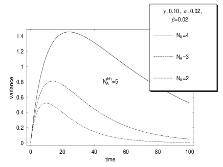
Figure 2: Time dependence of the variance of the number of $X$ particles in the case of $N_{A}<N_{A}^{(bf)}$.

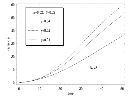
Figure 3: Time dependence of the variance of the number of $X$ particles in the case of $N_{A}>N_{A}^{(bf)}$ at different decay rate constants.

In order to have some insight into the nature of the time behavior of the variance of the number of autocatalytic particles we have calculated the variance ${\bf D}^{2}\{\xi(u)\}$ versus time curves for different values of the number of $A$ particles and for several decay rate constants $\gamma$. FIG. 2 shows the time dependence of ${\bf D}^{2}\{\xi(u)\}$ when $N_{A}<N_{A}^{(bf)}$ at a fixed value of rate constant. We see that the variance versus time curves have a maximum and after that they decrease slowly to zero.

In contrary to this, when $N_{A}>N_{A}^{(bf)}$, then the variance of the number of autocatalytic particles increase monotonously to infinity. It can be easily shown that

$$\lim_{u\rightarrow\infty}\frac{\mathbf{D}^{2}\{\xi(u)\}}{u}=\frac{1}{N_{A}}\frac{a}{a-b},$$

and so, we can use for large $u$ the asymptotic formula

$${\bf D}^{2}\{\xi(u)\}\approx\frac{1}{N_{A}}\frac{a}{a-b}\;u,\;\;\;\;\;\;u>>1.$$

The time dependence of the variance ${\bf D}^{2}\{\xi(u)\}$ in the case when $N_{A}>N_{A}^{(bf)}$ is seen in FIG. 3 for three decay rate constants. The variance converges to the infinity linearly with increasing time parameter, if $N_{A}>N_{A}^{(bf)}$, and to a constant value $b$, if $N_{A}=N_{A}^{(bf)}$, so we can say that the fluctuation of the number of $X$ particles in the stationary state near the ”bifurcation” point alters the possible conclusions based only on the average number of autocatalytic particles.

III Lifetime of the system

We say that a system is in the state ${\mathcal{S}}_{j}(t)$, when $\xi(t)=j$. Obviously, the system is live at time instant $t\geq 0$, when $\xi(t)>0$. Let us define the probability of transition ${\mathcal{S}}_{i}(t_{0})\rightarrow{\mathcal{S}}_{j}(t_{0}+t)$ by

$${\mathcal{P}}\{{\mathcal{S}}_{j}(t_{0}+t)|{\mathcal{S}}_{i}(t_{0})\}=p_{i,j}(t_{0}+t,t_{0}),\;\;\;\;\;\;\text{where}\;\;\;\;\;\;t\geq 0.$$ (43)

Since the process is homogenous in time $p_{i,j}(t_{0}+t,t_{0})=p_{i,j}(t)$, and using Eq. (8) we can write that

$$\frac{dp_{i,j}(t)}{dt}=-(\lambda_{j}+\mu_{j})\;p_{i,j}(t)+\lambda_{j-1}\;p_{i,j-1}(t)+\mu_{j+1}\;p_{i,j+1}(t),\;\;\;\;\;\;i,j=0,1,\ldots,$$ (44)

where

$$\lambda_{j}=jN_{X}\alpha,\;\;\;\;\;\;\mu_{j}=j[\beta(j-1)+\gamma].$$ (45)

We see that the first equation is

$$\frac{dp_{i,0}(t)}{dt}=\gamma p_{i,1}(t),$$ (46)

and the initial condition is given by $p_{i,j}(0)=\delta_{i,j}$. The random time $\theta_{n}$ due to the transition ${\mathcal{S}}_{n}(0)\rightarrow{\mathcal{S}}_{0}(\theta_{n}),\;n>0$ is the lifetime of the system which has been at $t=0$ in the state ${\mathcal{S}}_{n}(0)$. It is evident that

$${\mathcal{P}}\{\theta_{n}\geq t\}={\mathcal{P}}\{\xi(t)=0|\xi(0)=n\}=p_{n,0}(t)=H_{n}(t),$$

where $H_{n}(t)$ is the probability that the lifetime $\theta_{n}$ is not larger than $t$. The moments of the lifetime are given by

$$\mathbf{E}\{\theta_{n}^{k}\}=\int_{0}^{\infty}t^{k}\;dH_{n}(t),\;\;\;\;\;\;n>0\;\;\;\;\;\;\text{and}\;\;\;\;\;\;k=1,2,\ldots\;\;\;.$$ (47)

III.1 Extinction probability

The extinction of a system of state ${\mathcal{S}}_{n}(0)$ occurs when a transition to the state ${\mathcal{S}}_{0}(t)$ is realized for any $t\geq 0$. We define the extinction probability by

$$\lim_{t\rightarrow\infty}H_{n}(t)=L_{n},\;\;\;\;\;\;\forall\;n=1,2,\ldots,\;\;\;\;\;\;\text{and since}\;\;\;\;\;\;H_{n}(\infty)=p_{n,0}(\infty)=w_{0}$$

in accordance with (28) we find that

$$L_{n}=\left\{\begin{array}[]{ll}1,&\text{if $\gamma\neq 0$,}\\ \text{ }&\text{ }\\ 0,&\text{if $\gamma=0$,}\end{array}\right.\;\;\;\;\;\;\forall\;n=1,2,\ldots\;\;.$$ (48)

It is a remarkable result stating that a system being in any of states ${\mathcal{S}}_{n}(t_{0})$ at a given time instant $t_{0}$ after elapsing sufficiently long time $t>>t_{0}$ will be almost surly annihilated, if $\gamma\neq 0$, and never dies, i.e. the extinction probability is zero, if $\gamma=0$.

It is to mention that the statement (48) can be obtained from a nice lemma by Karlin karlin75 which can be formulated in the following way: introducing the notation

$$\rho_{k}=\prod_{j=1}^{k}\frac{\mu_{j}}{\lambda_{j}},$$ (49)

where $\mu_{j}$ and $\lambda_{j}$ are non-negative real numbers which are not necessarily equal to (45), it can be stated that if

$$K=\lim_{n\rightarrow\infty}\sum_{k=1}^{n}\;\rho_{k}=\infty,\;\;\;\;\;\;\text{then}\;\;\;\;\;\;L_{n}=1,\;\;\;\;\;\;\forall\;n=1,2,\ldots,$$ (50)

while if

$$K=\lim_{n\rightarrow\infty}\sum_{k=1}^{n}\;\rho_{k}<\infty,\;\;\;\;\;\;\text{then}\;\;\;\;\;\;L_{n}=\frac{\sum_{k=n}^{\infty}\rho_{k}}{1+\sum_{k=1}^{\infty}\rho_{k}}<1,\;\;\;\;\;\;\forall\;n=1,2,\ldots\;\;.$$ (51)

By using the expressions (45) we see immediately that

$$\rho_{k}=\prod_{j=1}^{k}\frac{\beta(j-1)+\gamma}{N_{A}\alpha}=\left(\frac{\beta}{N_{A}\alpha}\right)^{k}\;\frac{\Gamma(\gamma/\beta+j)}{\Gamma(\gamma/\beta)},$$

hence we can conclude that

$$K=\left\{\begin{array}[]{ll}\infty,&\text{if $\gamma\neq 0$,}\\ \text{ }&\text{ }\\ 0,&\text{if $\gamma=0$,}\end{array}\right.$$

and so, applying the lemma we prove the statement (48).

III.2 Average lifetime of the system

To determine the transition probability $p_{n,0}(t)$, i.e. the probability $H_{n}(t)$ is not an easy problem. Instead, we show how to calculate the average lifetime $\mathbf{E}\{\theta_{n}\}=\tau_{n}$. Let us define the parameters

$$\delta_{1}=\frac{1}{\mu_{1}},\;\;\;\;\;\;\text{and}\;\;\;\;\;\;\delta_{k}=\frac{\lambda_{1}\cdots\lambda_{k-1}}{\mu_{1}\cdots\mu_{k}},\;\;\;\;\;\;\text{if $k>1$},$$ (52)

and formulate the following statement called Karlin’s theorem karlin75 . If $\;\sum_{k=1}^{\infty}\delta_{k}<\infty$, then the average lifetime $\tau_{n}$ of a system containing $n$ autocatalytic particles is given by

$$\tau_{n}=\sum_{k=0}^{\infty}\delta_{k}+\sum_{j=1}^{n-1}\rho_{j}\;\sum_{k=j+1}^{\infty}\delta_{k},$$ (53)

where $\rho_{j}$ is defined by (49), and in contrary, if $\;\sum_{k=1}^{\infty}\delta_{k}=\infty$, then $\tau_{n}=\infty\;\;\forall\;n\geq 1.$ The proof of this statement can be found in Appendix B.

Now, by using this statement we would like to calculate the average lifetime of a system which is in the state ${\mathcal{S}}_{n}(t)$ at the moment $t$. Introducing the notations

$$a=\frac{N_{A}\alpha}{\beta}\;\;\;\;\;\;\text{and}\;\;\;\;\;\;b=\frac{\gamma}{\beta},$$ (54)

and by using the expressions (45) we can write

$$\delta_{j}=\frac{1}{\gamma}\left(\delta_{j,1}+(1-\delta_{j,1})\;\frac{a^{j-1}}{j\;(b+1)\cdots(b+j-1)}\right),$$ (55)

where $\delta_{j,1}$ is the Kronecker-symbol. Define the sum

$$d_{n}=\sum_{j=1}^{n}\delta_{j}=\frac{1}{\gamma}\left(1+\sum_{j=2}^{n}\frac{(j-1)!}{(b+1)\cdots(b+j-1)}\;\frac{a^{j-1}}{j!}\right)=\frac{\Gamma(b+1)}{\gamma}\;\sum_{j=1}^{n}\frac{a^{j-1}}{j\;\Gamma(b+j)},$$ (56)

for $n\geq 1$. If $\gamma\neq 0$, then one can see immediately that

$$\lim_{n\rightarrow\infty}d_{n}=\sum_{j=1}^{\infty}\delta_{j}<\infty,$$

i.e. the formula (53) should be used for the calculation of the average lifetime $\tau_{n}$.

First, determine $\tau_{1}$. It follows from Eq. (53) that

$$\tau_{1}=\sum_{j=1}^{\infty}\delta_{j}=\frac{\Gamma(b+1)}{\gamma}\;\sum_{j=1}^{\infty}\;\frac{a^{j-1}}{j\;\Gamma(b+j)}=\frac{1}{a\;\gamma}\;\int_{0}^{a}\Phi(1,b+1;u)\;du,$$ (57)

where $\Phi(1,b+1;u)$ is the confluent hypergeometric function. The next step is the calculation of the expression

$$s_{j}(a,b)=\rho_{j}\;\sum_{k=j+1}^{\infty}\delta_{k},$$

which can be rewritten into the form:

$$s_{j}(a,b)=\frac{1}{a^{j}}\;\prod_{i=1}^{j}(b+i-1)\;\sum_{k=j+1}^{\infty}\delta_{k}.$$

After some elementary algebra we obtain

$$s_{j}(a,b)=\frac{1}{\beta}\;\Gamma(b+j)\;\sum_{k=j+1}^{\infty}\frac{a^{k-j-1}}{k\;\Gamma(b+k)},$$

and finally we have

$$\tau_{n}=\tau_{1}+\frac{1}{\beta}\;\sum_{j=1}^{n-1}\Gamma(b+j)\;\sum_{k=j+1}^{\infty}\frac{a^{k-j-1}}{k\;\Gamma(b+k)}.$$ (58)

Introducing a new index $\ell=k-j$ we have

$$s_{j}(a,b)=\frac{1}{\beta}\;\Gamma(b+j)\sum_{\ell=0}^{\infty}\frac{a^{\ell}}{(j+\ell+1)\;\Gamma(b+j+\ell+1)},$$

which can be transformed into the expression

$$s_{j}(a,b)=\frac{1}{\beta}\;\frac{1}{a^{j+1}}\;\int_{0}^{a}v^{j-1}\;\sum_{\ell=0}^{\infty}\frac{(\ell+1)!\;\Gamma(b+j)}{\Gamma(b+j+\ell+1)}\;\frac{v^{\ell+1}}{(\ell+1)!}\;dv.$$

By using the identity

$$\sum_{\ell=0}^{\infty}\frac{(\ell+1)!\;\Gamma(b+j)}{\Gamma(b+j+\ell+1)}\;\frac{v^{\ell+1}}{(\ell+1)!}=\Phi(1,b+j;v)-1,$$

$s_{j}(a,b)$ takes a new form, namely

$$s_{j}(a,b)=\frac{1}{\beta}\;\frac{1}{a^{j+1}}\;\int_{0}^{a}v^{j-1}\;\left[\Phi(1,b+j;v)-1\right]\;dv.$$

Taking into account this formula the expression (58) can be rewritten in the form

$$\tau_{n}=\tau_{1}+\frac{1}{\beta}\;\sum_{j=1}^{n-1}\frac{1}{a^{j+1}}\;\int_{0}^{a}v^{j-1}\left[\Phi(1,b+j;v)-1\right]\;dv,$$ (59)

which is convenient for numerical calculations. From this equation we see that

$$\tau_{1}<\tau_{2}<\cdots<\tau_{n}<\cdots\;,$$

and we can prove the limit relation

$$\lim_{n\rightarrow\infty}\beta\;\tau_{n}<\infty.$$ (60)

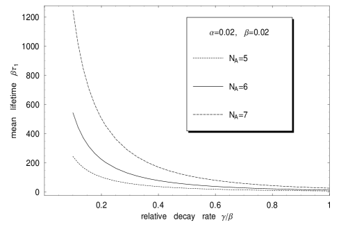
Figure 4: The mean value of the system lifetime vs. $\gamma/\beta$ at $N_{A}=5,6,7$, provided that the initial state of the system was ${\mathcal{S}}_{1}$.

It is necessary and sufficient to show that

$$\beta\;\lim_{n\rightarrow\infty}\sum_{j=1}^{n-1}s_{j}(a,b)<\infty.$$

Since $\Phi(1,b+j;v)-1$ is a non-negative, monotonously increasing function of $v\geq 0$ we can write immediately that

$$\beta s_{j}(a,b)\leq\frac{\Phi(1,b+j;a)-1}{a^{j+1}}\;\int_{0}^{a}v^{j-1}\;dv=\frac{\Phi(1,b+j;a)-1}{a\;j},$$

and if $j\geq 1$, then

$$\Phi(1,b+j;a)-1=\sum_{k=1}^{\infty}\frac{a^{k}}{(b+j)(b+j+1)\cdots(b+j+k-1)}\leq\sum_{k=1}^{\infty}\frac{a^{k}}{j\;(j+1)(j+2)\cdots(j+k-1)}\leq\frac{a}{j}\;e^{a},$$

consequently, we obtain the inequality

$$\beta\;\lim_{n\rightarrow\infty}\sum_{j=1}^{n-1}s_{j}(a,b)<e^{a}\;\sum_{j=1}^{\infty}\frac{1}{j^{2}}=\frac{\pi^{2}}{6}\;e^{a}<\infty,$$

and this proves the statement (60).

We calculated how the mean value $\tau_{1}$ depends on the ratio $\gamma/\beta$ at three different values of the number of $A$ particles. The results are shown in FIG. 4. We can see that $\beta\tau_{1}$ decreases rapidly with increasing $\gamma/\beta$, and if the values $\gamma/\beta$ are smaller than $0.4$, then we can observe that the larger is the number $N_{A}$ in the system the longer is the average lifetime $\beta\tau_{1}$.

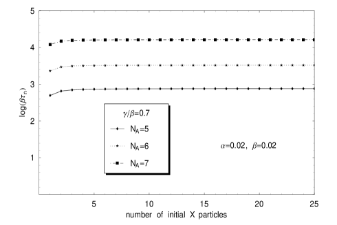
Figure 5: Dependence of the logarithm of the mean value of the system lifetime on the number of $X$ particles to be found in the system at that time moment which the lifetime is counted from.

That FIG. 5 shows is rather surprising. The mean value of the system lifetime does not depend practically on the number of $X$ particles to be found in the system at that time moment which the lifetime is counted from. We can state that the average lifetime of systems controlled by reactions (1) is already determined by several ${X}$ particles, and even a large increase of the number of ${X}$ particles does not effect significantly on the system lifetime.

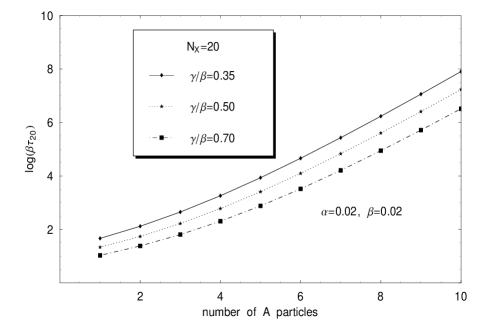
Figure 6: Dependence of the logarithm of the mean value $\beta\;\tau_{20}$ on the number of $A$ particles at three different values of $\gamma/\beta$.

On this basis imagine an ”organism” which consists of ${X}$ particles capable of self-reproduction and self-annihilation. Assume that the organism becomes dead if it loses the last ${X}$ particle. One might think that the greater is the number of ${X}$ particles in the organism the larger is irs average lifetime. Contrary to this conviction, an organism containing, let us say $500$ particles hardly lives longer than that which contains only $10$ particles. By using the values $N_{A}=7,\;\beta=0.02$ and $\gamma=0.014$ we obtain that $\beta\tau_{10}\approx 67.21$ and $\beta\tau_{500}\approx 67.351$. It is rather surprising that the increase is only $0.21\%$.

In FIG. 6 we see the dependence of the logarithm of the mean value $\beta\;\tau_{20}$ on the number of $A$ particles at three different $\gamma/\beta$. One can observe that the increase of $N_{A}$ results in a rather large lengthening of the average lifetime, i.e. the effect of the substrate particles on the process is much stronger than that of the autocatalytic particles.

IV Conclusions

We assumed the distribution of reacting particles in the system volume to be uniform and introduced the notion of the point model of reaction kinetics. In this model the probability of a reaction between two particles per unit time is evidently proportional to the product of their actual numbers. By using this assumption we constructed a stochastic model for systems controlled by the reactions $A+X\rightleftharpoons X+X,\;\;X\rightarrow B$ provided that the number of $A$ particles is kept constant by a suitable reservoir, and the end-product particles $B$ do not take part in the reaction.

We have shown that the stochastic model results in an equation for the expectation value $m_{1}(t)$ of autocatalytic particles $X$ which differs strongly from the kinetic rate equation. Further, we found that if the decay constant $\gamma$ of the particles $X$ is not zero, then the stochastic description, in contrary to the rate equation description, brings about only one stationary state with probability $1$, and it is the zero-state ${\mathcal{S}}_{0}$ . It has been also proven that the probability of a nonzero stationary state is larger than zero, if and only if the decay rate constant is equal to zero. Consequently, the average number of $X$ particles in the stationary state is larger than zero, if only $\gamma=0$. However, one has to underline that this average number is completely different from that which corresponds to the law of the mass action of reversible chemical reactions.

We paid a special attention on the random behavior of the system lifetime, and derived an exact formula for the average lifetime. It has been shown that the mean value of the system lifetime does not depend practically on the number of $X$ particles to be found in the system at the time instant which the lifetime is counted from. For example, the lifetime of a system having $500$ $X$ particles at the beginning is larger only by $0.2$% than the lifetime of a system containing $10$ $X$ particles at the time moment $t=0$.

Appendix A Eigenvalues of the matrix $\mathbf{A}$

As mentioned already, the eigenvalues of a normal Jacobi matrix are real and different. We would like to prove the following theorem:

Theorem. The $\nu=0$ is an eigenvalue of the normal Jacobi matrix ${\bf A}$ defined by (15) and the other nonzero eigenvalues are all negative.

Proof. Denote by $a_{ij},\;\;i,j\in{\mathcal{Z}}_{+}$  the elements of matrix $\mathbf{A}$. We see immediately that

$$\sum_{i}a_{ij}=C_{j-1}-D_{j}+B_{j+1}=0,$$ (61)

i.e. the sum of elements of any column of the matrix $\mathbf{A}$ is equal to zero. Strictly speaking, the theorem itself is a straightforward consequence of this property. If $\nu$ an eigenvalue, then

$$\sum_{j}a_{ij}x_{j}=\nu x_{i},$$

and $x_{0},x_{1},\ldots,x_{i},\ldots$ define a nonzero eigenvector

$$\vec{x}=\left(\begin{array}[]{c}x_{0}\\ x_{1}\\ \vdots\\ x_{j}\\ \vdots\end{array}\right).$$

Let $\vec{y}$ be an arbitrary nonzero vector and form the following expression:

$$\sum_{i}\;\sum_{j}a_{ij}x_{j}y_{i}=\nu\sum_{i}x_{i}y_{i}=\nu\sum_{j}x_{j}y_{j},$$

which can be rewritten in the form

$$\sum_{j}x_{j}\left(\sum_{i}a_{ij}y_{i}-\nu y_{j}\right)=0.$$

This equality can be valid only if

$$\sum_{i}a_{i,j}y_{i}=\nu y_{j},$$ (62)

and because $\vec{y}$ is an arbitrary nonzero vector one can chose its components to be equal to unity. Then taking into account the property (61) one has

$$\nu=\sum_{i}a_{i,j}=0,$$

i.e. $\nu=0$ is indeed an eigenvalue.

Now, we show if $\nu\neq 0$, then $\nu<0$. Since $a_{jj}\leq 0$, and $a_{ij}\geq 0$, if $i\neq j$, it follows from (62) that

$$\sum_{i\neq j}a_{ij}y_{i}=\left(|a_{jj}|+\nu\right)y_{j}.$$ (63)

As $\vec{y}$ is an arbitrary nonzero vector, let us chose it so that

$$|y_{j}|=\max_{i}|y_{i}|=q>0,\;\;\;\;\;\;\text{and since}\;\;\;\;\;\;\sum_{i\neq j}a_{ij}=|a_{jj}|,$$

we obtain the inequality

$$\sum_{i\neq j}a_{ij}y_{i}\leq\sum_{i\neq j}a_{ij}q=q|a_{jj}|.$$

Taking into account the relation (63) we have

$$q|a_{jj}|\geq\left(|a_{jj}|+\nu\right)q$$

which can be valid only if $\nu<0$. Q.E.D.

Appendix B Karlin’s theorem

Theorem. If $\;\sum_{k=1}^{\infty}\delta_{k}<\infty$, then the average lifetime $\tau_{n}$ of a system containing $n$ autocatalytic particles is given by

$$\tau_{n}=\sum_{k=0}^{\infty}\delta_{k}+\sum_{j=1}^{n-1}\rho_{j}\;\sum_{k=j+1}^{\infty}\delta_{k},$$ (64)

where $\rho_{j}$ is defined by (49), and in contrary, if $\;\sum_{k=1}^{\infty}\delta_{k}=\infty$, then $\tau_{n}=\infty\;\;\forall\;n\geq 1.$

Proof. Assume the system to be in the state ${\mathcal{S}}_{n}$ at a given time instant $t$ and suppose that the first reaction after $t$ occurs at a random time moment $t+\vartheta_{n}$. This reaction can result in a transition to either the state ${\mathcal{S}}_{n-1}$ or ${\mathcal{S}}_{n+1}$ with probabilities

$$\frac{\mu_{n}}{\lambda_{n}+\mu_{n}}\;\;\;\;\;\;\;\text{and}\;\;\;\;\;\;\frac{\lambda_{n}}{\lambda_{n}+\mu_{n}},$$

respectively. Since $t$ is arbitrary, the equation

$$\theta_{n}=\vartheta_{n}+\frac{\mu_{n}}{\lambda_{n}+\mu_{n}}\;\theta_{n-1}+\frac{\lambda_{n}}{\lambda_{n}+\mu_{n}}\;\theta_{n+1}$$ (65)

is valid with probability $1$. Taking into account that

$${\mathcal{P}}\{\vartheta_{n}\geq t\}=1-\exp\{-(\lambda_{m}+\mu_{n})t\},$$

one obtains from (65) the recursion

$$\tau_{n}=\frac{1}{\lambda_{n}+\mu_{n}}+\frac{\mu_{n}}{\lambda_{n}+\mu_{n}}\;\tau_{n-1}+\frac{\lambda_{n}}{\lambda_{n}+\mu_{n}}\;\tau_{n+1},$$ (66)

where $\tau_{0}=0$. Introducing the difference $\omega_{n}=\tau_{n}-\tau_{n+1}$ after simple rearrangements we obtain

$$\omega_{n}=\frac{1}{\lambda_{n}}+\frac{\mu_{n}}{\lambda_{n}}\;\omega_{n-1},$$ (67)

the solution of which can be written in the form:

$$\omega_{n}=\frac{1}{\lambda_{n}}+\sum_{i=1}^{n-1}\frac{1}{\lambda_{i}}\;\prod_{j=i+1}^{n}\frac{\mu_{j}}{\lambda_{j}}+\omega_{0}\;\prod_{j=1}^{n}\frac{\mu_{j}}{\lambda_{j}}.$$

By using the notation

$$\delta_{i}=\left\{\begin{array}[]{ll}\frac{1}{\mu_{1}},&\text{if $i=1$,}\\ \text{ }&\text{ }\\ \frac{\lambda_{1}\cdots\lambda_{i-1}}{\mu_{1}\cdots\mu_{i}},&\text{if $i>1$. }\end{array}\right.$$

and taking into account the identity

$$\left(\sum_{i=1}^{n}\delta_{i}\right)\;\prod_{j=1}^{n}\frac{\mu_{j}}{\lambda_{j}}=\frac{1}{\lambda_{n}}+\sum_{i=1}^{n-1}\frac{1}{\lambda_{i}}\;\prod_{j=i+1}^{n}\frac{\mu_{j}}{\lambda_{j}},$$

and the relation $\omega_{0}=\tau_{1}$, we have

$$(\tau_{n}-\tau_{n+1})\;\prod_{j=1}^{n}\frac{\lambda_{j}}{\mu_{j}}=\sum_{i=1}^{n}\delta_{i}-\tau_{1}.$$ (68)

If $\lim_{n\rightarrow\infty}\sum_{i=1}^{n}\delta_{i}={\mathcal{D}}=\infty$, then $\tau_{n}=\infty,\;\;\forall\;\;n\geq 1$ i.e. the average lifetime of the system is infinite. The proof is simple: it is obvious that $\tau_{n}<\tau_{n+1}$, therefore, it follows from (68) that $\sum_{i=1}^{n}\delta_{i}<\tau_{1}$ for any $n$, and if $n\rightarrow\infty$, than $\tau_{1}$ must be infinite. Since $\tau_{n}<\tau_{n+1}\;\;\forall\;n\geq 1$, it is evident that $\tau_{n}=\infty,\;\;\forall\;\;n\geq 1$, hence the statement is proven.

If $\lim_{n\rightarrow\infty}\sum_{i=1}^{n}\delta_{i}={\mathcal{D}}<\infty$, then one can find a finite real number $K$ such that $\prod_{i=1}^{n}(\lambda_{i}/\mu_{i})<K$, consequently

$$\lim_{n\rightarrow\infty}(\tau_{n}-\tau_{n+1})\;\prod_{i=1}^{n}\frac{\lambda_{i}}{\mu_{i}}=0,$$

and it follows from this that

$$\tau_{1}=\sum_{i=1}^{\infty}\delta_{i}.$$ (69)

Taking into account this relation we can rewrite Eq. (68) into the form:

$$(\tau_{n}-\tau_{n+1})\frac{1}{\rho_{n}}=\sum_{i=n+1}^{\infty}\delta_{i},$$

where $\rho_{n}$ is defined by (49). Introducing the notation

$$\chi_{n}=\sum_{i=n}^{\infty}\delta_{i},$$ (70)

we have

$$\tau_{n+1}=\tau_{n}+\rho_{n}\;\chi_{n+1},$$

the solution of which is nothing else than

$$\tau_{n}=\tau_{1}+\sum_{j=1}^{n-1}\rho_{j}\;\chi_{j+1},$$

and by substituting $\tau_{1}$ and $\chi_{j+1}$ we obtain immediately the equation (64).

References

- (1) L. Pál, arXiv:cond-mat/0404402
- (2) V.M. Parmon, Vest. RAS, 72, 976 (2002)
- (3) D. Segré, Y. Pilpel, D. Lancet, Physica A, 249, 558 (1998)
- (4) P.F. Stadler, W. Fontana, J.H. Miller, Physica D, 63, 378 (1993)
- (5) S. Karlin and H.M. Taylor: A First Course in Stochastic Processes, (Academic Press, New York, 1975)