Vortex Lattice Structure of Fulde-Ferrell-Larkin-Ovchinnikov Superconductors

Abstract

In superconductors with singlet pairing, the inhomogeneous Fulde-Ferrell-Larkin-Ovchinnikov (FFLO) state is expected to be stabilized by a large Zeeman splitting. We develop an efficient method to evaluate the Landau-Ginzburg free energies of FFLO-state vortex lattices and use it to simplify the considerations that determine the optimal vortex configuration at different points in the phase diagram. We demonstrate that the order parameter spatial profile is completely determined, up to a uniform translation, by its Landau level index $n$ and the vortex Lattice structure and derive an explicit expression for the order parameter spatial profile that can be used to determine $n$ from experimental data.

I introduction

Forty years ago Fulde and Ferrellff , and Larkin and Ovchinnikovlo proposed that a superconducting state with an inhomogeneous order parameter would become stable when a singlet superconductor is disturbed by Zeeman splitting between electrons with opposite spin orientations. The Zeeman splitting can be due to either an external magnetic field or an internal exchange field. In spite of ongoing theoretical interestreview in the Fulde-Ferrell-Larkin-Ovchinnikov(FFLO) state, evidence for its occurrence has been sparse until recently. The situation has been changed by experimental results suggestive of the FFLO state in organic, heavy-fermion, and possibly other unconventional supercondcutors gloos ; modler ; tachiki ; geg ; singleton ; radovan ; bianchi ; martin . Recent experimental results on the heavy fermion compound CeCoIn₅, a quasi-two-dimensional d-wave superconductor, are particularly compellingradovan ; bianchi ; martin . Independently, speculations that the FFLO state may also be realized in high density quark matter have caught the attention of the particle physics communityreview , adding to the flurry of interest in this uncommon superconducting state.

To establish the presence of the FFLO state unambiguously one needs to perform a phase sensitive experiment that detects order parameter oscillations and measures their wavelength. One possible phase sensitive probe based on the Josephson effect between a FFLO superconductor and a BCS superconductorya was proposed some time ago by Yang and Agterberg. Although conceptually straightforward this experiment is yet to be carried out, possibly due to technical difficulties in its implementation. More recently, there has been interest in the vortex lattice structure (VLS) of an FFLO state subjected to an orbital magnetic field, and particularly in the possibility of using the character of the VLS to infer the presence of an underlying FFLO superconductorsr ; krs ; hb ; hbbm ; klein . The key ideabul is that, depending on the interplay between the orbital and Zeeman effects of the magnetic field, the order parameter of a FFLO state near its upper critical field can correspond to a high Landau level (LL) index Cooper pair wave function. Recent worksr ; krs ; hb ; hbbm ; klein on the FFLO VLS in specific situations has demonstrated that these high LL index VLS’s can be very different from the triangular lattice Abrikosov VLS favored by lowest Landau level (LL) Cooper pairs. The case of FFLO states in an orbital field is the only example known to us in which bosons (Cooper pairs in the present case) are placed in high LLs; the absence of a fermionic Pauli exclusion principle implies that one cannot force bosons to occupy a high LL simply by increasing the particle density. Electronic states in high LLs have recently been found to exhibit physicselectron that can be quite different from that found in the lowest LL, suggesting that surprises might also occur in high LL bosonic physics.

In this paper we apply techniques developed in studies of electronic states in a strong magnetic field (primarily motivated by the quantum Hall effectgirvin ) to study the vortex states of FFLO superconductors. Using these techniques, we develop a very efficient method to determine the VLS implied by a given Ginsburg-Landau free energy functional. As established by previous studiessr ; krs ; hb ; hbbm ; klein , the VLS is highly non-universal; we argue here that the VLS approaches a universal limit near the tricritical point, in the sense that the structure near this point in the phase diagram depends on the LL index of the order parameter only. We determine the VLS in this limit explicitly. We demonstrate that the order parameter spatial profile is completely determined, up to a uniform translation, by its Landau level index $n$ and by the VLS, and derive an explicit expression for the order parameter spatial profile that can be used to determine $n$ from experimental data. If the LL index can be determined by comparing experimental and theoretical VLSs, the order parameter momentum in the absence of a field can also be determined.

We lay out the theoretical method we have developed in the following section, and present the VLSs suggested by its application in section III. These techniques may be useful in addressing other aspects of high Landau level bosonic physics in FFLO superconductors or elsewhere. In section IV we summarize our results and make a comparison with related recent work.

II Theoretical method

To address FFLO VLS physics we follow a Ginzburg-Landau approach similar to that of Refs.hb, ; hbbm, . The free-energy density appropriate for the FFLO state, has the formbk :

$$F \propto|(-\nabla^{2}-q^{2})\psi|^{2}+a|\psi|^{2}+b|\psi|^{4}+c|\psi|^{2}|\nabla\psi|^{2}$$ (1)

$$+ d[(\psi^{*})^{2}(\nabla\psi)^{2}+\psi^{2}(\nabla\psi^{*})^{2}]+e|\psi|^{6},$$

where $a,b,c,d,e$ and $q$ are parameters that depend on both temperature and Zeeman splitting. The free energy of Eq.(1) is appropriate for an s-wave superconductor with completely isotropic gap and band dispersion, the case we will consider here. Anisotropy in either pairing interaction or single electron dispersion will lead to additional termsay . The fundamental difference between FFLO and BCS superconductors is expressed by the first term in $F$ which describes the kinetic energy of the order parameter; in an FFLO superconductor this term is minimized when the order parameter carries a finite wave vector (or momentum) $q$; in a BCS superconductor $q=0$. Thus far we have only taken into account the Zeeman effect of the external magnetic field, which is appropriate for the case of a two-dimensional superconductor with an external magnetic field parallel to the plane. For a 3D superconductor or for a 2D superconductor with the field ${\bf B}$ tilted out of system plane, orbital coupling must be accounted for by performing a minimal substitution $\nabla\psi\rightarrow{\bf D}\psi=(\nabla-2ie{\bf A}/c)\psi$ with $\nabla\times{\bf A}=B_{\perp}\hat{z}$. It is the 2D case that we have in mind here because it allows the Zeeman field, which controls $q$ and the other LG model parameters, and the field $B_{\perp}$ to be controlled independently.

To find the order parameter $\psi$ that minimizes the free energy of the system near a continuous phase transition, one first determines the Cooper pair Landau level index that minimizes the coefficient of the quadratic terms in Eq. (1). The eigenvalues of ${\bf D}^{2}=(\nabla-2ie{\bf A}/c)^{2}$ are $-(2n+1)/\ell^{2}$, where $\ell=\sqrt{\hbar c/2eB}$ is the Cooper pair magnetic length and $n=0,1,2,\cdots$ is the LL index. For a BCS superconductor the kinetic energy is minimized by $n=0$, i.e., $\psi$ is a lowest LL wave function. For a FFLO superconductor, however, the kinetic energy is minimized by the index $n$ that minimizes $|(2n+1)/\ell^{2}-q^{2}|$. The optimal value of $n$ will be large when $B_{\perp}$ is small.bul

Because of the macroscopic degeneracy of a Landau level, the order parameter retains considerable freedom at $B_{\perp}\neq 0$ even when $n$ is fixed. As we explain below, this freedom is resolved by minimizing the remaining terms of Eq. (1) with a properly normalized wave function $\psi({\bf r})$; this corresponds to optimizing the vortex lattice. The overall magnitude of the order parameter is determined by balancing quadratic and higher order terms in the GL energy functional. For a BCS superconductor that is described by an ordinary Ginsburg-Landau theory for which $n=0$ and in which the $|\psi|^{4}$ term is the only addition term, it is known that the optimal VLS is triangular. In the following we use techniques developed in studies of the quantum Hall effect to derive expressions for and understand the relationships between the higher order terms present in Eq. (1).

We assume that the VLS is that of a Bravais lattice so that there is one flux quantum per unit cell. The central quantity in our calculation is the Fourier transform of $|\psi({\bf r})|^{2}$: $\int{d^{2}{\bf r}}|\psi({\bf r})|^{2}e^{-i{\bf k}\cdot{\bf r}}$. Since $|\psi({\bf r})|^{2}$ is periodic, this integral is zero unless ${\bf k}={\bf G}$, where ${\bf G}$ is a reciprocal lattice vector of the vortex lattice. For ${\bf k}={\bf G}$, we define

$$\tilde{\Delta}_{\bf G}=\int_{u.c.}{d^{2}{\bf r}}|\psi({\bf r})|^{2}e^{-i{\bf G}\cdot{\bf r}}=\langle\psi|e^{-i{\bf G}\cdot{\bf r}}|\psi\rangle.$$ (2)

Here $\int_{u.c.}$ stands for integration within a unit cell of the vortex lattice, and we assume that $\psi({\bf r})$ is normalized within a unit cell so that

$$\int_{u.c.}{d^{2}{\bf r}}|\psi({\bf r})|^{2}=\langle\psi|\psi\rangle=1.$$ (3)

To proceed, we introduce the guiding center coordinatehaldane

$${\bf R}={\bf r}+\ell^{2}\hat{z}\times(-i\nabla+(2e/c){\bf A}),$$ (4)

and separate ${\bf r}$ into ${\bf r}={\bf R}+({\bf r}-{\bf R})$. It is knowngirvin that the guiding center ${\bf R}$ has no matrix element between states in different LLs, while $({\bf r}-{\bf R})$ changes the LL index of a state without changing its guiding center dependence; as a consequence components of ${\bf R}$ and $({\bf r}-{\bf R})$ commute with each otherhaldane .

Two key observations simplify the calculations below. First $|\psi\rangle$ is an eigenket of $e^{-i{\bf G}\cdot{\bf R}}$. It follows that $\Delta_{\bf G}$ is the eigenvalue of this operator and, since the operator is unitary, must be a phase factor. As we discuss later the phase factor can be fixed by a convenient choice of spatial origin. The operator $\exp(-i{\bf G}\cdot{\bf R})$ results in a translation by ${\bf G}\ell^{2}\times\hat{z}$ in real space, which is a direct lattice vector, and multiplication by a phase factor that is gauge but not position dependent. The most straightforward way to prove this property is to construct $\psi({\bf r})$ explicitly in a convenient gauge (say the Landau gauge), show that it is true in this gauge, and that an arbitrary gauge transformation (on $\psi({\bf r})$ and $e^{-i{\bf G}\cdot{\bf R}}$ simultaneously) does not change the result. The second key observations follows from the fact that ${\bf r}-{\bf R}$ does not act on guiding center coordinates:

$$\langle\psi|e^{-i{\bf G}\cdot({\bf r}-{\bf R})}|\psi\rangle=L_{n}(G^{2}\ell^{2}/2)e^{-G^{2}\ell^{2}/4}$$ (5)

for any normalized $n$-th Landau level state. (Here $L_{n}(x)$ is the Laguerre polynomial.)

It follows from the above properties that

$$\tilde{\Delta}_{\bf G} = \langle\psi|e^{-i{\bf G}\cdot{\bf r}}|\psi\rangle=\langle\psi|e^{-i{\bf G}\cdot{\bf R}}|\psi\rangle\langle\psi|e^{-i{\bf G}\cdot({\bf r}-{\bf R})}|\psi\rangle$$ (6)

$$= \Delta_{\bf G}L_{n}(G^{2}\ell^{2}/2)e^{-G^{2}\ell^{2}/4},$$

with $|\Delta_{\bf G}|=1$. Eq. (6) allows for a very straightforward calculation of the Abrikosov factor

$$\beta^{(n)}_{A} = A\int_{u.c.}{d^{2}{\bf r}}|\psi({\bf r})|^{4}=\sum_{\bf G}|\tilde{\Delta}_{\bf G}|^{2}$$ (7)

$$= \sum_{\bf G}[L_{n}(G^{2}\ell^{2}/2)]^{2}e^{-G^{2}\ell^{2}/2},$$

where $A=2\pi\ell^{2}$ is the area of the unit cell which contains one flux quantum. In Eq. (7) the VLS is characterized by its reciprocal lattice vectors ${\bf G}$. For BCS superconductors described by ordinary Ginsburg-Landau free energy functional, the VLS is determined by minimizing $\beta^{(0)}_{A}$;saint it is known that in the lowest LL ($n=0$), $\beta^{(0)}_{A}$ is minimized by the triangular lattice with $\beta^{(0)}_{A}=1.1596$,saint a result easily reproduced using Eq. (7), with the choice ${\bf G}=m{\bf g}_{1}+n{\bf g}_{2}$, where ${\bf g}_{1}=(\sqrt{4\pi/\sqrt{3}}/\ell)\hat{x}$ and ${\bf g}_{2}=(\sqrt{\pi/\sqrt{3}}/\ell)\hat{x}+(\sqrt{\sqrt{3}\pi}/\ell)\hat{y}$ are the basis vectors of the (reciprocal) triangular lattice. For the square lattice, we have ${\bf g}_{1}=(\sqrt{2\pi}/\ell)\hat{x}$ and ${\bf g}_{2}=(\sqrt{2\pi}/\ell)\hat{y}$, which yields $\beta^{(0)}_{A}=1.1803$, also in agreement with previously known results.saint

To determine the VLS of a FFLO superconductor one needs to take into account the fact that the LL index $n$ is not necessarily zero and the presence of contributions from terms other than $|\psi({\bf r})|^{4}$ in the free energy functional (1). These can be done straightforwardly using extensions of Eq. (7) that also follow from the separation of guiding-center dependence in the appropriate operators. For example the contribution from the $|\psi|^{6}$ term is parametrized by

$$\gamma^{(n)}_{A} = A^{2}\int_{u.c.}{d^{2}{\bf r}}|\psi({\bf r})|^{6}=\sum_{{\bf G}_{1}{\bf G}_{2}}\tilde{\Delta}_{{\bf G}_{1}}\tilde{\Delta}_{{\bf G}_{2}}\tilde{\Delta}_{-{\bf G}_{1}-{\bf G}_{2}}$$ (8)

$$= \sum_{{\bf G}_{1}{\bf G}_{2}}\Delta_{{\bf G}_{1}}\Delta_{{\bf G}_{2}}\Delta_{-{\bf G}_{1}-{\bf G}_{2}}e^{-(G_{1}^{2}+G_{2}^{2}+{\bf G}_{1}\cdot{\bf G}_{2})\ell^{2}/2}$$

$$\times L_{n}(G_{1}^{2}\ell^{2}/2)L_{n}(G_{2}^{2}\ell^{2}/2)L_{n}(|{\bf G}_{1}+{\bf G}_{2}|^{2}\ell^{2}/2)$$

$$= \sum_{{\bf G}_{1}{\bf G}_{2}}\cos[\hat{z}\cdot({\bf G}_{1}\times{\bf G}_{2})\ell^{2}/2]e^{-(G_{1}^{2}+G_{2}^{2}+{\bf G}_{1}\cdot{\bf G}_{2})\ell^{2}/2}$$

$$\times L_{n}(G_{1}^{2}\ell^{2}/2)L_{n}(G_{2}^{2}\ell^{2}/2)L_{n}(|{\bf G}_{1}+{\bf G}_{2}|^{2}\ell^{2}/2),$$

where we used the property

$$e^{-i({\bf G}_{1}+{\bf G}_{2})\cdot{\bf R}}=e^{-i{\bf G}_{1}\cdot{\bf R}}e^{-i{\bf G}_{2}\cdot{\bf R}}e^{i\hat{z}\cdot({\bf G}_{1}\times{\bf G}_{2})\ell^{2}/2},$$ (9)

which follows from the commutator between different components of ${\bf R}$haldane : $[R_{x},R_{y}]=i\ell^{2}$. It follows that

$$\Delta_{-{\bf G}_{1}-{\bf G}_{2}}=\Delta^{-1}_{{\bf G}_{1}}\Delta^{-1}_{{\bf G}_{2}}e^{i\hat{z}\cdot({\bf G}_{1}\times{\bf G}_{2})\ell^{2}/2}.$$ (10)

Similarly, using the fact that $\psi$ is an eigenfunction of the operator $(\nabla-2ie{\bf A}/c)^{2}$, the contributions from the $c$ and $d$ terms in Eq. (1) can be expressed as combinations of $\beta^{(n)}_{A}$ andhb

$$I^{(n)}_{22}=\int_{u.c.}{d^{2}{\bf r}}|\psi({\bf r})|^{2}|{\bf D}\psi({\bf r})|^{2}.$$ (11)

To evaluate $I^{(n)}_{22}$, we introduce

$$\lambda_{\bf G} = \int_{u.c.}{d^{2}{\bf r}}|{\bf D}\psi({\bf r})|^{2}e^{-i{\bf G}\cdot{\bf r}}$$ (12)

$$= -\int_{u.c.}{d^{2}{\bf r}}\psi^{*}{\bf D}[{\bf D}\psi({\bf r})e^{-i{\bf G}\cdot{\bf r}}]$$

$$= -\int_{u.c.}{d^{2}{\bf r}}\psi^{*}[{\bf D}^{2}\psi({\bf r})-i({\bf G}\cdot{\bf D})\psi({\bf r})]e^{-i{\bf G}\cdot{\bf r}}.$$

It is easy to show using the fact that $\psi$ is an eigen wavefunction of ${\bf D}^{2}$ that the second term in the final line of Eq. (12) does not contribute to the integral. We thus find

$$\lambda_{\bf G}=(2n+1)\tilde{\Delta}_{\bf G}/\ell^{2},$$ (13)

and

$$I^{(n)}_{22}=\sum_{\bf G}\tilde{\Delta}_{\bf G}\lambda_{-{\bf G}}=(2n+1)\beta^{(n)}_{A}/\ell^{2}.$$ (14)

We have thus found that $I^{(n)}_{22}$ is proportional to $\beta^{(n)}_{A}$; in particular, they have exactly the same dependence on the VLS. This fact simplifies the determination of the optimal VLS significantly.

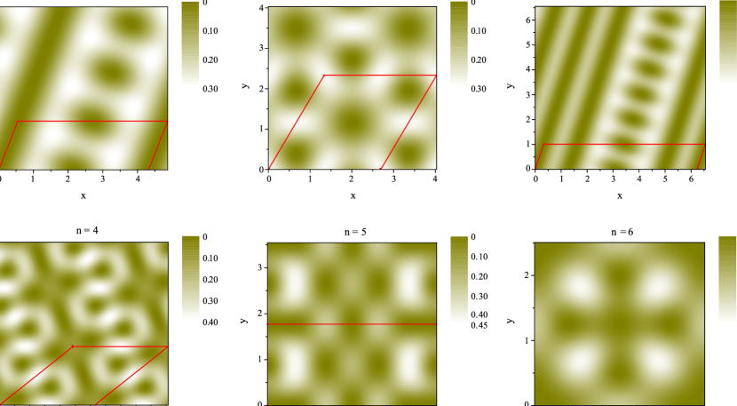
Figure 1: (Color online) Plots of the square of order parameter magnitude that minimizes $\beta_{A}^{(n)}$, for Landau levels $0<n\leq 6$. The lines (when present) indicate the region of a unit cell of the vortex lattice. Lengths are in unit of the magnetic length $\ell$.

III Results

In tables I and II we have listed the VLS that minimizes $\beta^{(n)}_{A}$ and $\gamma^{(n)}_{A}$ respectively, for the order parameter in the $n$th Landau level. Fig. 1 contains plots for small Landau level indices of the square of the order parameter magnitude for the vortex lattices that minimize $\beta^{(n)}_{A}$. For $n=0$ we find that that both $\beta_{A}$ and $\gamma_{A}$ are minimized by the triangular lattice, in agreement with previously known resultssaint ; hb . Evidently the situation changes drastically for $n\neq 0$. The competition between different potential VLS’s can be understood in terms of the simple reciprocal lattice expression of $\beta^{(n)}_{A}$, Eq. (7). For $n=0$, the Laguerre polynomial is $L_{n=0}(x)\equiv 1$, so it is clear that $\beta_{A}$ is minimized by placing the reciprocal lattice vectors (${\bf G}$’s) as far away from the origin as possible given the fixed unit cell area, which is what a triangular lattice does. For $n\geq 1$, on the other hand, $L_{n}(x)$ is a polynomial with nodes whose positions depend on $n$; one may thus lower $\beta^{(n)}_{A}$ by, for example, choosing ${\bf G}$’s such that $L_{n}(G^{2}\ell^{2}/2)$ is close to zero for some reciprocal lattice vectors, leading to very non-standard VLSs under most circumstances. Similar considerations apply to the optimal VLS that minimizes $\gamma^{(n)}_{A}$. Overall, the optimal values of both $\beta^{(n)}_{A}$ and $\gamma^{(n)}_{A}$ increase with $n$, reflecting the fact that the order parameter wave function becomes increasingly oscillatory (and therefore less uniform) as $n$ increases. For $n=1$ and $3$ VLS’s are characterized by order parameter concentration in widely spaced stripe-like regions with rapid but weak longitudinal modulations. The stripes are characterized by lines with definite guiding centers and odd parity perpendicular quantum wave functions, yielding a series of lines along which the order parameter is small. For even $n$ and for larger $n$ the optimal VLS’s tend to be more close-packed, with lattices that are close to square occurring frequently.

LL index	0	1	2	3	4	5	6
aspect ratio	1	0.36	1	0.17	1	0.50	1
angle $\theta$	$\pi/3$	1.21	1.05	1.26	0.69	$\pi/2$	$\pi/2$
$\beta^{(n)}_{A}$	1.16	1.32	1.20	1.43	1.38	1.42	1.44

Table 1: The optimal vortex lattice structure that minimizes $\beta^{(n)}_{A}$ in different Landau levels. The vortex lattice structure is parametrized by the aspect ratio between the two basis vectors, and the angle between them.

LL index	0	1	2	3	4	5	6
aspect ratio	1	0.39	1	0.16	1	1	1
angle $\theta$	$\pi/3$	1.53	1.04	1.10	0.68	$\pi/3$	$\pi/2$
$\gamma^{(n)}_{A}$	1.42	1.89	1.57	2.29	2.19	2.31	2.47

Table 2: The optimal vortex lattice structure that minimizes $\gamma^{(n)}_{A}$ in different Landau levels. The vortex lattice structure is parametrized by the aspect ratio between the two basis vectors, and the angle between them.

Since both the quartic terms ($b,c$ and $d$ terms in Eq. (1)) and the sixth order term (the $e$ term) contribute to the total free energy, and $\beta^{(n)}_{A}$ and $\gamma^{(n)}_{A}$ depend on the lattice structure in different ways for $n\geq 1$, the optimal VLS will depends on an interplay between the two, and is therefore non-universal; this is very different from the Abrikosov lattice of the BCS superconductor, which is always triangular. In the following we discuss two limiting cases in which the optimal VLS approaches a universal limit, in the sense that it depends on the Landau level index $n$ only.

(i) It is knownbk that at the tricritical point which occurs for $T\approx 0.56T_{c}$ (the maximum temperature at which the FFLO state is stable) both the order parameter wave vector $q$ and the coefficient of the quartic term $b$ vanish. Near this tricritical point, the contributions of the quartic terms to the free energy vanishes (the terms proportional to $c$ and $d$ both involve gradients are proportional to $q^{2}$). The optimal VLS is therefore determined by minimizing $\gamma^{(n)}_{A}$ alone and is given by the entries listed in table II.

(ii) Along the $H_{c2}$ line, the transition can be either first order or second order. The transition is second order when the combined contribution to the free energy from the quartic terms is positive, in which case the contribution from sixth order term is negligible near the phase boundary, due to the smallness of the order paramter. As shown above, the contribution to the free energy from all the quartic terms is proportional to $\beta^{(n)}_{A}$ with lattice structure independent prefactors. Minimizing the free energy is therefore equivalent to minimizing $\beta^{(n)}_{A}$, resulting in an optimal VLS that depends on $n$ only and given in this case by the entries listed in table I. There is, however, an important caveat in this case since the conclusion is reached based on the free energy Eq. (1), in which quartic terms that involve more gradients are neglected; these terms are in principle comparable to the terms kept, because the order parameter wavevector $q$ is finite, and it may not be possible to express their contributions in terms of $\beta^{(n)}_{A}$ alone. These terms do not affect case (i) however because $q$ approaches zero there.

Once the VLS is determined, one can obtain the detailed spatial dependence of the order parameter in the $n$th LL by counter-Fourier transform Eq. (2):

$$|\psi({\bf r})|^{2} = {1\over 2\pi\ell^{2}}\sum_{\bf G}\tilde{\Delta}_{\bf G}e^{-i{\bf G}\cdot{\bf r}}$$ (15)

$$= {1\over 2\pi\ell^{2}}\sum_{\bf G}\Delta_{\bf G}L_{n}(G^{2}\ell^{2}/2)e^{-G^{2}\ell^{2}/4}e^{i{\bf G}\cdot{\bf r}}.$$

By parameterizing the reciprocal lattice vector ${\bf G}=m_{1}{\bf g}_{1}+m_{2}{\bf g}_{2}$ where ${\bf g}_{1}$ and ${\bf g}_{2}$ are the two basis vectors of the reciprocal lattice, while $m_{1}$ and $m_{2}$ are two integers, we find

$$\Delta_{\bf G}=\langle\psi|e^{-i(m_{1}{\bf g}_{1}+m_{2}{\bf g}_{2})\cdot{\bf R}}|\psi\rangle=e^{im_{1}m_{2}\hat{z}\cdot({\bf g}_{1}\times{\bf g}_{2})\ell^{2}/2}$$ (16)

$$\times \langle\psi|e^{-im_{1}{\bf g}_{1}\cdot{\bf R}}e^{-im_{2}{\bf g}_{2}\cdot{\bf R}}|\psi\rangle=(-1)^{m_{1}m_{2}}e^{i(m_{1}\theta_{1}+m_{2}\theta_{2})},$$

where $e^{i\theta_{1}}$ and $e^{i\theta_{2}}$ are the eigen values of $e^{-i{\bf g}_{1}\cdot{\bf R}}$ and $e^{-i{\bf g}_{2}\cdot{\bf R}}$ respectively; we may choose $\theta_{1}=\theta_{2}=0$ by selecting the spatial origin in the unit cell. We thus obtain

$$|\psi({\bf r})|^{2} = {1\over 2\pi\ell^{2}}\sum_{m_{1}m_{2}}(-1)^{m_{1}m_{2}}L_{n}(|m_{1}{\bf g}_{1}+m_{2}{\bf g}_{2}|^{2}\ell^{2}/2)$$ (17)

$$\times e^{-|m_{1}{\bf g}_{1}+m_{2}{\bf g}_{2}|^{2}\ell^{2}/4}\cos[(m_{1}{\bf g}_{1}+m_{2}{\bf g}_{2})\cdot{\bf r}].$$

Experimentally one can determine the VLS (and thus ${\bf g}_{1}$ and ${\bf g}_{2}$), by neutron or muon scattering for example, while the magnitude of the local order parameter (or gap) may be measured by STM. By comparing the measured results with Eq. (17) one may be able to determine the LL index $n$. This allows for an estimate of the order parameter wavevector in the absence of the orbital magnetic field: $q\approx\sqrt{2n+1}/\ell$, which is an alternative to measuring $q$ using the Josephson effectya . It is important however to keep the following caveats in mind when making this comparison. (i) We have assumed here that the order parameter wave function is in a given Landau level exclusively. This is true only when one is very close to the portions of $H_{c2}$ line where the transition is second order, or to the tricritical point mentioned above. Away from these regions mixing of different Landau levels becomes increasingly important, and this can affect our results significantly. (ii) Our analysis is based on a Ginsburg-Landau free energy that is completely isotropic. Real systems often have some anisotropy, due to either the pairing interaction (as in a d-wave superconductor) or single-electron dispersion (band structure effect). It should be possible however to generalize our methods to anisotropic cases.

IV Summary

In this work we have presented and applied an efficient method to determine the vortex lattice structure (VLS) of an FFLO superconductor, based on an appropriate Ginsburg-Landau free energy functional. In our approach all calculations are performed in a completely gauge independent manner. We have shown that the VLS is universal in certain limiting cases, in the sense that it depends on the Landau level index of the order parameter only. Independent of the VLS, which is not universal in the general case, our results enable an experimental determination of the Landau level index which follows from the constraints on spatial structure that exist when only guiding center degrees of freedom are available. Given the Landau level index, one can estimate the order parameter wavevector in the absence of orbital magnetic field.

Fundamentally, our approach is similar to that used in Refs. hb, ; hbbm, in that it is based on minimizing an appropriate Ginsburg-Landau free energy functional. The efficiency of the new calculational technique, however, allows one to determine the vortex lattice structure for a wide range of parameters, instead of only the specific cases studied earlier. Our methods can be applied to any problem in which bosons occupy high Landau levels. In addition to vortex states of FFLO superconductors, another possibility is bosonic cold atoms in a rotating trap with an optical lattice potential that has been engineered to have the minimum band energy away from the zone center.

In a recent paper,klein Klein studied the VLS of FFLO superconductors starting directly from a weak-coupling BCS model (which is a generalization of earlier work by Eilenbergereilenberger ), instead of using a Ginsburg-Landau free energy functional. In his work the VLS was determined solely from the terms that are quartic in the order parameter in the free energy, while as we see here terms beyond quartic can be crucial in certain regimes. On the other hand it appears that he was able to evaluate the quartic terms without using a gradient expansion, which appears to be an improvement on the usual Ginsburg-Landau approach; this might be important under some circumstances. We note that we find the dependence of VLS on the Landau level index $n$ appears to be quite complicated, without any obvious indication of the simplification in the limit $n\rightarrow\infty$, suggested in Ref. klein, .

- (1) P. Fulde and A. Ferrell, Phys. Rev. 135, A550 (1964).
- (2) A. I. Larkin and Yu. N. Ovchinnikov, Sov. Phys. JETP 20, 762 (1965).
- (3) For a review, see R. Casalbuoni and G. Nardulli, Rev. Mod. Phys. 76, 263 (2004).
- (4) K. Gloos, R. Modler, H. Schimanski, C. D. Bredl, C. Geibel, F. Steglich, A. I. Buzdin, N. Sato, and T. Komatsubara, Phys. Rev. Lett. 70, 501 (1993).
- (5) R. Modler, P. Gegenwart, M. Lang, M. Deppe, M. Weiden, T. Lühmann, C. Geibel, F. Steglich, C. Paulsen, J. L. Tholence, N. Sato, T. Komatsubara, Y. Onuki, M. Tachiki and S. Takahashi, Phys. Rev. Lett. 76, 1292 (1996).
- (6) M. Tachiki, S. Takahashi, P. Gegebwart, M. Weiden, M. Lang, C. Geibel, F. Steglich, R. Modler, C. Paulsen, and Y. Onuki, Z. Phys. B 100, 369 (1996).
- (7) P. Gegebwart, M. Deppe, M. Koppen, F. Kromer, M. Lang, R. Modler, M. Weiden, C. Geibel, F. Steglich, T. Fukase, and N. Toyota, Ann. Physik 5, 307 (1996).
- (8) J. Singleton, J. A. Symington, M.-S. Nam, A. Ardavan, M. Kurmoo, and P. Days, J. Phys. Condens. Matter 12, L641 (2000).
- (9) H.A. Radovan, N.A. Fortune, T.P. Murphy, S.T. Hannahs, E.C. Palm, S.W. Tozer, and D. Hall, Nature 425, 51 (2003).
- (10) A. Bianchi, R. Movshovich, C. Capan, P. G. Pagliuso, and J. L. Sarrao, Phys. Rev. Lett. 91, 187004 (2003).
- (11) C. Martin, C. C. Agosta, S. W. Tozer, H. A. Radovan, E. C. Palm, T. P. Murphy, J. L. Sarrao, cond-mat/0309125.
- (12) K. Yang and D. F. Agterberg, Phys. Rev. Lett. 84, 4970 (2000). A related experiment was proposed in L. Bulaevskii, A. Buzdin and M. Maley, Phys. Rev. Lett. 90, 067003 (2003).
- (13) H. Shimahara and D. Rainer, J. Phys. Soc. Jpn. 66, 3591 (1997).
- (14) U. Klein, D. Rainer, and H. Shimahara, J. Low. Temp. Phys. 118, 91 (2000).
- (15) M. Houzet and A. Buzdin, Europhys. Lett. 50, 375 (2000).
- (16) M. Houzet, A. Buzdin, L. Bulaevskii, and M. Maley, Phys. Rev. Lett. 88, 227001 (2002).
- (17) U. Klein, Phys. Rev. B 69, 134518 (2004).
- (18) L. N. Bulaevskii, Sov. Phys. JETP 38, 634 (1974).
- (19) M. M. Fogler, A. A. Koulakov, and B. I. Shklovskii, Phys. Rev. B 54, 1853 (1996); R. Moessner and J. T. Chalker, Phys. Rev. B 54, 5006 (1996); M. P. Lilly, K. B. Cooper, J. P. Eisenstein, L. N. Pfeiffer, and K. W. West, Phys. Rev. Lett. 82, 394 (1999). R. R. Du, D. C. Tsui, H. L. Stormer, L. N. Pfeiffer, K. W. Baldwin, and K. W. West, Solid State Commun. 109, 389 (1999); E. H. Rezayi, F. D. M. Haldane, and K. Yang, Phys. Rev. Lett. 83, 1219 (1999); F.D.M. Haldane, E H. Rezayi, and K. Yang, Phys. Rev. Lett. 85, 5396 (2000).
- (20) The Quantum Hall Effect, 2nd Ed., edited by R. E. Prange and S. M. Girvin (Springer, New York, 1990).
- (21) A. I. Buzdin and H. Kachkachi, Phys. Lett. A 225, 341 (1997).
- (22) D. F. Agterberg and K. Yang, J. Phys.: Condens. Matter 13, 9259 (2001).
- (23) See, e.g., F. D. M. Haldane, in Ref.girvin, ; A.H. MacDonald in Proceedings of the Les Houches Summer School on Mesoscopic PhysicsElsevierAmsterdam1995edited by E. Akkermans, G. Montambeaux, and J.-L. Pichard.
- (24) See, e.g., D. Saint-James, G. Sarma and E. J. Thomas (eds.), Type II Superconductors, Pergamon Press, New York (1969).
- (25) G. Eilenberger, Z. Physik 190, 142 (1966); Phys. Rev. B 153, 584 (1967).