Linear-scaling quantum Monte Carlo with
non-orthogonal localized orbitals

Abstract

We have reformulated the quantum Monte Carlo (QMC) technique so that a large part of the calculation scales linearly with the number of atoms. The reformulation is related to a recent alternative proposal for achieving linear-scaling QMC, based on maximally localized Wannier orbitals (MLWO), but has the advantage of greater simplicity. The technique we propose draws on methods recently developed for linear-scaling density functional theory. We report tests of the new technique on the insulator MgO, and show that its linear-scaling performance is somewhat better than that achieved by the MLWO approach. Implications for the application of QMC to large complex systems are pointed out.

The quantum Monte Carlo (QMC) technique [1] is becoming ever more important in the study of condensed matter, with recent applications including the reconstruction of semiconductor surfaces [2], the energetics of point defects in insulators [3], optical excitations in nanostructures [4], and the energetics of organic molecules [5]. Although its demands on computer power are much greater than those of widely used techniques such as density functional theory (DFT), its accuracy is also much greater for most systems. With QMC now being applied to large complex systems containing hundreds of atoms, a major issue is the scaling of the required computer effort with system size. In other electronic-structure techniques, including DFT, the locality of quantum coherence [6] suggests that it should generally be possible to achieve linear-scaling, or $O(N)$ operation, in which the computer effort is proportional to the number of atoms $N$. Very recently, a procedure has been suggested [7] for achieving at least partial linear scaling for QMC, based on the idea of “maximally localized Wannier functions” [8]. The purpose of this report is to propose and test a simpler alternative method, which appears to have important advantages.

The $O(N)$ techniques that have been developed for tight binding (TB) [9], DFT [10, 11] and Hartree-Fock [12] calculations all depend ultimately on the fact that the density matrix $\rho({\bf r},{\bf r}^{\prime})$ associated with the single-electron orbitals decays to zero as $|{\bf r}-{\bf r}^{\prime}|\rightarrow\infty$, and the manner of this decay has been extensively studied ([13] and references therein). Briefly, the decay is algebraic for metals and exponential for insulators, with the decay rate increasing with band gap, so that there is more to be gained from $O(N)$ techniques for wide-gap insulators. Equivalently, the extended orbitals used in most conventional techniques can be linearly combined to form localized orbitals, which again decay exponentially in insulators. (For a review of early localized-orbital methods in quantum chemistry, see Ref. [14].) Orthogonal Wannier functions are one form of localized orbitals, but it has long been recognized that stronger localization can be achieved by going to non-orthogonal orbitals, as is done in many existing $O(N)$ TB, DFT and quantum-chemistry techniques.

In QMC, the trial many-body wavefunction $\Psi_{\rm T}({\bf r}_{1},\ldots{\bf r}_{N})$ consists of a Slater determinant $D$ of single-electron orbitals $\psi_{n}({\bf r}_{i})$ multiplied by a parameterized Jastrow correlation factor $J({\bf r}_{1},\ldots{\bf r}_{N})$. (In the pseudopotential-based QMC of interest here, the $\psi_{n}({\bf r}_{i})$ are commonly taken from a plane-wave pseudopotential DFT calculation.) In variational Monte Carlo (VMC), $J$ is ‘optimized’ by varying its parameters so as to reduced the variance of the ‘local energy’ $\Psi_{\rm T}^{-1}\left(\hat{H}\Psi_{\rm T}\right)$, where $\hat{H}$ is the many-electron Hamiltonian. Since VMC by itself is not usually accurate enough, the optimized $\Psi_{\rm T}$ produced by VMC is used in diffusion Monte Carlo (DMC), which achieves the exact ground state within the fixed nodal structure imposed by the Slater determinant $D$. In conventional DMC, a large fraction of the computer time goes into evaluating the single-electron orbitals for all the electron positions ${\bf r}_{i}$ in each of the replicas (QMC “walkers”). For this part of the calculations, the number of computer operations required to perform each QMC step scales at least as $N^{2}$ ($M$ orbitals $\psi_{n}({\bf r}_{i})$ for $N$ positions ${\bf r}_{i}$, with $M$ proportional to $N$), and the scaling deriorates to $N^{3}$ if (as is often done) a plane-wave basis set is used to represent the $\psi_{n}({\bf r}_{i})$. The memory requirement scales as $N^{2}$, and this also places important limits on the size of system that can be treated.

As pointed out by Williamson et al. [7], the scaling for the evaluation of the $\psi_{n}({\bf r}_{i})$ can be reduced from $N^{3}$ or $N^{2}$ to $N$ if the Slater determinant $D$ is re-expressed in terms of localized orbitals, which themselves are represented in terms of localized basis functions. The key point here is that a determinant is changed by at most a constant overall factor if arbitrary linear combinations of its rows or columns are made. More precisely, if we construct orbitals $\phi_{m}({\bf r})$ as linear combinations

$$\phi_{m}({\bf r})=\sum_{n=1}^{M}c_{mn}\psi_{n}({\bf r})\;,\;\;\;\;\;m=1,\,2,\,\ldots\,M$$ (1)

of the original single-electron orbitals $\psi_{n}({\bf r})$, then the determinant ${\rm det}\,|\phi_{m}({\bf r}_{i})|$ is given by:

$${\rm det}\,|\phi_{m}({\bf r}_{i})|={\rm det}\,|c_{mn}|\,.\,{\rm det}\,|\psi_{n}({\bf r}_{i})|\;.$$ (2)

This means that the determinants ${\rm det}\,|\phi_{m}({\bf r}_{i})|$ and ${\rm det}\,|\psi_{n}({\bf r}_{i})|$ are exactly the same functions of the $M$ electronic positions $\{{\bf r}_{i}\}$, apart from the constant factor ${\rm det}\,|c_{mn}|$, so that, provided the transformation matrix $||c_{mn}||$ is non-singular, the orbitals $\phi_{m}({\bf r}_{i})$ yield precisely the the same total energy in QMC as the $\psi_{n}({\bf r})$. It is important to appreciate that the linear combinations need not constitute a unitary transformation, so that the orbitals $\phi_{m}({\bf r})$ can be non-orthogonal. The additional freedom gained by dispensing with orthogonality can be exploited to improve the localization of the orbitals.

These ideas lead to the following simple and general scheme. Let $\psi_{n}({\bf r})$ be any set of $M$ orbitals, which in general extend over the entire volume $\Omega$ of the cell containing the atoms, and let there be a region $\omega$ of arbitrary shape contained in $\Omega$. We wish to find the linear combination $\phi({\bf r})=\sum_{n=1}^{M}c_{n}\psi_{n}({\bf r})$ such that $\phi({\bf r})$ is maximally localized in $\omega$. We interpret this to mean that the $c_{n}$ are varied so as to maximize the quantity $P$ defined by:

$$P=\int_{\omega}d{\bf r}\,|\phi({\bf r})|^{2}\left/\int_{\Omega}d{\bf r}\,|\phi({\bf r})|^{2}\right.\;,$$ (3)

where the integrals go over the regions $\omega$ and $\Omega$ respectively. We refer to $P$ as the localization weight, and note that by definition $0\leq P\leq 1$. Now $P$ can be re-expressed as:

$$P=\sum_{m,n}c_{m}^{\star}A_{mn}^{\omega}c_{n}\left/\sum_{m,n}c_{m}^{\star}A_{mn}^{\Omega}c_{n}\right.\;,$$ (4)

where:

$$A_{mn}^{\omega}=\int_{\omega}d{\bf r}\,\psi_{m}^{\star}\psi_{n}\;,\;\;\;\;\;A_{mn}^{\Omega}=\int_{\Omega}d{\bf r}\,\psi_{m}^{\star}\psi_{n}\;.$$ (5)

Clearly $P$ takes its maximum value when the $c_{n}$ are the components of the eigenvector of the generalized eigenvalue equation:

$$\sum_{n}A_{mn}^{\omega}c_{n}=\lambda_{\alpha}\sum_{n}A_{mn}^{\Omega}c_{n}$$ (6)

associated with the largest eigenvalue $\lambda_{1}$, and this maximum value of $P$ is equal to $\lambda_{1}$. More generally, the $s$ most localized linear combinations in $\omega$ are associated with the $s$ largest eigenvalues $\lambda_{\alpha}$ ($\alpha=1,\ldots s$), where the $\lambda_{\alpha}$ are ordered in descending sequence.

The idea is now to use this scheme to produce $M$ localized orbitals $\phi_{m}({\bf r})$, which are used instead of the $M$ extended orbitals $\psi_{n}({\bf r})$ in the determinant $D$. We do this by choosing a number $\nu_{\rm reg}$ of localization regions, and taking the $p_{\rm loc}$ most localized orbitals in each of these regions, so that $M=\nu_{\rm reg}p_{\rm loc}$ is equal to the number of orbitals $\psi_{n}({\bf r})$. If no approximations are made, the results thus obtained in both VMC and DMC will be identical to those obtained with the $\psi_{n}$. But now we can obtain $O(N)$ scaling by truncating the $\phi_{m}({\bf r})$ so that they are exactly zero outside their localization regions. Provided the $\phi_{m}({\bf r})$ have almost all their weight inside their regions, the only effect of this truncation will be to introduce a slight shift of the nodal surfaces, so that DMC results will come out essentially identical to those obtained with the conventional $O(N^{2})$ scheme. This gives $O(N)$ scaling because it makes the determinant $|\phi_{m}({\bf r}_{i})|$ sparse. Specifically, for a given electron position ${\bf r}_{i}$, the number of orbitals $\phi_{m}$ for which $\phi_{m}({\bf r}_{i})$ is non-zero is no longer the total number of orbitals, but is proportional to the number of localization regions that contain ${\bf r}_{i}$. This is $O(1)$, rather than $O(N)$, and the number of operations needed for orbital evaluation is reduced by a factor equal to the ratio of the localization volume to the volume of the whole system.

To implement this method, we need to consider carefully the basis used for representing the $\phi_{m}({\bf r})$ and the $\psi_{n}({\bf r})$. This basis must be large enough and flexible enough to represent them very accurately, while at the same time representing the truncated $\phi_{m}({\bf r})$ everywhere without introducing computationally troublesome discontinuities. To achieve linear scaling, it is also vital that the basis functions be localized. Fortunately, this problem of representing localized orbitals has already been extensively studied within $O(N)$ DFT [15, 16, 17, 18]. We adopt here the B-spline (also called ‘blip-function’) representation used in the conquest $O(N)$ DFT code [10, 18]. The blip functions consist of localized cubic splines centred on the points of a regular grid, each function being non-zero only inside a region extending two grid spacings in each direction from its centre. Details of the blip representation, its close relationship with the plane-wave basis, and its efficiency in representing both extended and localized functions have been described elsewhere [19].

We have tested our method on the prototypical oxide material MgO in the rock-salt structure at ambient pressure. Because of its large band gap (experimental $E_{\rm g}=7.7$ eV), this kind of material should be particularly suited to $O(N)$ methods. The QMC calculations were performed using the appropriately modified casino code [20] on a supercell of 64 atoms, with extended orbitals $\psi_{n}({\bf r})$ at the $\Gamma$-point obtained from a DFT plane-wave calculation in the local-density approximation. Hartree-Fock pseudopotentials were used. Since MgO is a highly ionic material, the valence electrons are associated almost entirely with the anions, so that it is natural to take localization regions associated with the O ions. We take four localized orbitals $\phi_{m}({\bf r})$ for each O ion. The simplest procedure is to localize all four orbitals in the same region centred on the O site, this region being either spherical or cubic. We then expect to find one most localized orbital, corresponding roughly to an O 2s state, and three next most localized orbitals, corresponding roughly to the three 2p states. However, another way of thinking about localization is to seek four equivalent hybrid sp³-like orbitals. If we do this, it is natural to take four separate localization regions for each O, one for each sp³-like orbital. With this alternative procedure, to preserve the symmetry between the four orbitals, we take the centres of the regions to be displaced by a distance $d$ from the O site along four tetrahedral directions, and we keep only the single most localized orbital in each region. The distance $d$ can be chosen to optimize the localization weight.

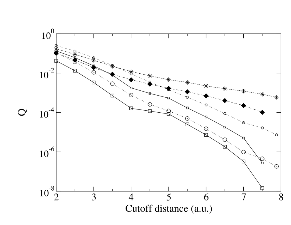
Figure 1: Dependence of localization weight on cut-off distance for bulk MgO. Quantity plotted is $Q\equiv 1-P$, where $P$ is localization weight defined by eqn (3). Large and small open circles: spherical cut-off for s-like and p-like localized orbitals; large and small open squares: cubic cut-off for s-like and p-like localized orbitals. Solid diamonds and stars: cubic and spherical cut-off for maximally localized Wannier orbitals.

In order for our method to succeed, the localized orbitals $\phi_{m}({\bf r})$ must be strongly localized (localization weight $P$ very close to unity) in regions having reasonably small cut-off radii. Fig. 1 compares the calculated localization weights $P$ (the quantity plotted is actually $Q\equiv 1-P$) with those of the maximally localized Wannier functions produced by the scheme of Ref. [7] for both cubic and spherical regions. We note that the results shown for our method were obtained with localization regions centred on O sites, while the Wannier results were obtained with displaced centres. In spite of this, our $\phi_{m}({\bf r})$ are remarkably strongly localized, even for cut-off radii as small as 6 a.u. The decay of $Q$ to zero is much more rapid for non-orthogonal orbitals, as expected. Also expected is the more rapid decay in both methods if cubic, rather than spherical regions are used. We have done tests also on the localization weight in our method when the localization centres are displaced, and we find that a displaced distance of $d=0.66$ a.u. works well. The main effect of this is to reduce $Q$ for all four orbitals to roughly the value for the s-like orbital in Fig. 1.

for the p-like orbitals to essentially the value obtained for the s-like orbitals.

Given the excellent localization, the key question is now the convergence of the VMC and DMC total energies obtained in our $O(N)$ scheme towards the ‘exact’ values obtained with extended orbitals. We show in Fig. 2 the total energy per atom obtained in VMC from calculations using spherical and cubic cut-offs and with localization centres on O sites and on displaced sites. As expected, convergence is somewhat more rapid with cubic regions, though the difference is not large. There is a considerable improvement with displaced localization centres. With this procedure, the total energy agrees with the ‘exact’ value already within $\sim 10$ meV/atom when the localization radius is 6 a.u., and even for a radius of 4.5 a.u. the agreement is only slightly worse. For comparison, we show results obtained with orthogonal Wannier orbitals, these orbitals being on displaced centres. We note that the total energy converges considerably less rapidly. With spherical regions, the energy still differs from the ‘exact’ value by at least 20 meV even with a radius of 7.5 a.u., which is almost half the cell length. Timings on our scheme show, as expected, that the time for evaluation of non-zero orbitals $\phi_{m}({\bf r}_{i})$ is proportional to the ratio of the localization volume to the volume of the whole cell. For example, if we go from a cubic localization region having a radius of 7.8 a.u. to a spherical region of radius 6 a.u., the time for orbital evaluation decreases by a factor of roughly $(4\pi 6^{3}/3)/(2\times 7.8)^{3}\simeq 0.25$.

We have also done tests on the performance of our linear-scaling method for DMC. We show in Fig. 3 the total energy per atom for MgO from DMC calculations using a localization region centred on the O sites. As with the VMC tests, the energy appears to be converged within $\sim 10$ meV/atom for a cut-off radius of 6 a.u. As in the case of VMC, the time for orbital evaluation is proportional to the localization volume.

We have therefore demonstrated that a precision of 10 meV/atom, which is considerably better than is needed for most purposes, is achieved with remarkably small localization regions. Even though our tests have all been done on a single system size, we can be sure that $O(N)$ scaling is achieved, because the reduction in the number of operations is proportional to the ratio of the localization volume to the volume of the whole system.

An additional and important gain from the type of $O(N)$ QMC proposed here is the large factor by which the memory requirement is reduced. This factor is also roughly the ratio between the volume of the localization region and the volume of the whole system. With the rather small MgO system of 64 ions used for the present tests, and a spherical localization cut-off of 6 a.u., the memory is reduced by a factor of 4. But QMC calculations on extended matter frequently needs systems of up to 10 times this size, so that the memory requirement will often be reduced by well over an order of magnitude. Although the number of operations needed for orbital evaluation is also reduced by this factor, at present the overall gain is less dramatic, since other parts of the QMC calculation (Ewald calculation of Coulomb energy, manipulation of determinants, etc) may account for up to 50 % of the time. Nevertheless, this still means a halving of the computation time for large systems, even if these other parts of QMC are left as they are. However, as pointed out earlier [7], $O(N)$ operation should be achievable for these other parts too.

We also note that the techniques we have described may be the key to constructing QMC ‘embedding’ methods, in which QMC is used to treat a spatially localized part of an extended system (e.g. a defect or a surface), while the rest of the system is treated either by using a matched technique of lower precision, or by invoking $O(N)$ QMC information on the bulk. The close relationship between the $O(N)$ problem and the embedding problem has been pointed out elsewhere [21] in the context of tight-binding and DFT calculations.

The oxide system we have used for the present practical tests has the special feature of a large band gap. It goes without saying that useful $O(N)$ operation will not be so easily obtained for metals and narrow-gap semiconductors. However, large areas of materials physics and chemistry, as well as bio-materials and aqueous systems, involved wide-gap materials, so we expect $O(N)$ QMC to be very widely applicable. In oxide science, problems where the new method should be immediately applicable include the energetics of bulk defects, perfect and defective surfaces and the adsorption of molecules at these surfaces, where the deficiencies and limitations of standard DFT methods are well known. We are currently preparing to attempt such calculations on MgO systems.

In conclusion, we have proposed and tested a new technique for achieving linear scaling in one of the most demanding parts of QMC calculations. In addition to being simpler and more robust than an earlier technique, it appears also to be more efficient. The new technique already makes it possible to treat large systems that would be out of reach of conventional QMC methods. Research areas where the technique is immediately applicable include defects and surfaces of oxide materials, and molecular processes on these surfaces.

DA acknowledges support from the Royal Society, and also thanks the Leverhulme Trust and the CNR for support. The authors are indebted to R.J. Needs, M.D. Towler and N.D. Drummond for advice and technical support in the use of the casino code, and for providing us with the pseudopotentials used in this work.

Figure 2: Convergence of linear-scaling VMC total energy per atom to value obtained with extended orbitals for bulk MgO. Open circles and squares: present method with spherical and cubic cut-offs, for localized orbitals centred on O sites. Filled circles and squares: spherical and cubic cut-offs, for displaced localized orbitals. Filled diamonds and stars: maximally localized Wannier orbitals with cubic and spherical cut-offs. Horizontal dashed line shows total energy/atom obtained with extended orbitals.

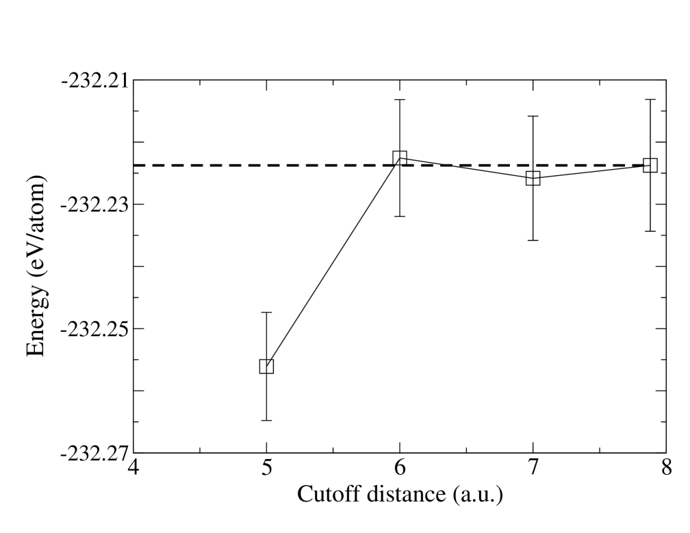
Figure 3: Convergence of linear-scaling DMC total energy per atom to value obtained with extended orbitals for bulk MgO. Open squares with statistical error bars: present with cubic cut-off. Dashed line shows result with extended orbitals.

References

- [1] Foulkes W M C, Mitas L, Needs R J and Rajagopal G 2001 Rev. Mod. Phys. 73 33
- [2] Healy S B, Filippi C, Kratzer P, Penev E and Scheffler M 2001 Phys. Rev. Lett. 87 016105
- [3] Hood R Q, Kent P R C, Needs R J and Briddon P R 2003 Phys. Rev. Lett. 91 076403
- [4] Williamson A J, Grossman J C, Hood R Q, Puzder A and Galli G 2002 Phys. Rev. Lett. 89 196803
- [5] Aspuru-Guzik A, El Akramine O, Grossman J C and Lester W A 2004 J. Chem. Phys. 120 3049
- [6] Kohn W 1996 Phys. Rev. Lett. 76 3168
- [7] Williamson A J, Hood R Q and Grossman J C 2001 Phys. Rev. Lett. 87 246406
- [8] Marzari N and Vanderbilt D 1997 Phys. Rev. B 56 12847
- [9] Bowler D R, Aoki M, Goringe C M, Horsfield A P and Pettifor D G 1997 Modell. Simul. Mater. Sci. Eng. 5 199
- [10] Bowler D R, Miyazaki T and Gillan M J 2002 J. Phys.: Condens. Matter 14 2781
- [11] Soler J M, Artacho E, Gale J D, Garcia A, Junquera J, Ordejon P and Sanchez-Portal D 2002 J. Phys.: Condens. Matter 14 2745
- [12] Challacombe M 1999 J. Chem. Phys. 110 2332
- [13] Ismail-Beigi S and Arias T A 1999 Phys. Rev. Lett. 82 2127
- [14] Stoneham A M 1975 Theory of Defects in Solids, Oxford University Press, Oxford, Sec. 7.5
- [15] Mostofi A A, Skylaris C K, Haynes P D and Payne M C 2002 Comput. Phys. Commun. 147 788
- [16] Gan C K, Haynes P D and Payne M C 2001 Phys. Rev. B 63 205109
- [17] Fattebert J L and Bernholc J 2000 Phys. Rev. B 62 1713
- [18] Hernández E, Gillan M J and Goringe C M 1996 Phys. Rev. B 53 7147
- [19] Hernández E, Gillan M J and Goringe C M 1997 Phys. Rev. B 55 13485
- [20] Needs R J, Towler M D, Drummond N D and Kent P R C 2004 ‘casino Version 1.7 User Manual’, University of Cambridge, Cambridge
- [21] Bowler D R and Gillan M J 2002 Chem. Phys. Lett. 355 306