Current and noise in a model of an AC-STM molecule-metal junction

Abstract

The transport properties of a simple model for a finite level structure (a molecule or a dot) connected to metal electrodes in an alternating current scanning tunneling microscope (AC-STM) configuration is studied. The finite level structure is assumed to have strong binding properties with the metallic substrate, and the bias between the STM tip and the hybrid metal-molecule interface has both an AC and a DC component. The finite frequency current response and the zero frequency photo-assisted shot noise are computed using the Keldysh technique, and examples for a single site molecule (a quantum dot) and for a two-site molecule are examined. The model may be useful for the interpretation of recent experiments using an AC-STM for the study of both conducting and insulating surfaces, where the third harmonic component of the current is measured. The zero frequency photo-assisted shot noise serves as a useful diagnosis for analyzing the energy level structure of the molecule. The present work motivates the need for further analysis of current fluctuations in electronic molecular transport.

I Introduction

The understanding of electronic transport phenomena in molecule-electrode interfaces is a key element of any technological realization of the potential of single-molecule electronics[1, 2]. The basic physics governing the current voltage characteristics in the coherent regime is reasonably well understood in terms of generalizations of the Landauer model where current is viewed as a quantum scattering problem and the effect of the electrodes is included via a self-energy contribution. Such a model has been successfully used to interpret data from both isolated molecules in STM, AFM and break junctions experiments[3, 4, 5], as well as experiments on Self Assembled Monolayers[6, 7, 8]. Most experiments on molecular-scale devices have been carried out on a two-terminal assembly, but measurements have also been reported in gated systems[9, 10]. A vast majority of experimental and theoretical studies have focused on the measurement of the current in such molecular junctions. Generally speaking, in the coherent tunneling regime, the zero frequency current $I(0)$ in molecular wire junctions depends on the electronic structure of the extended molecule-electrode system, the spatial profile of the voltage drop, the electro-chemical potential across the junction and the self-energy of the contacts that contains the information about the coupling between the finite molecule and the extended electrode[11, 12]. Yet from the point of view of mesoscopic physics, the current alone is not sufficient to fully characterize the transport: the second moment of the current – the noise – has been shown to provide crucial information concerning the effective charge of the carriers and their statistics[13, 14]. While noise measurements still represent a certain challenge in molecular transport – as experiments are typically performed with tunnel contacts – recently noise was computed for simple molecules using a Hückel type Hamiltonian [15, 16] and in the case of Coulomb interaction in the molecule using an Anderson impurity model[17]. The present work deals with the computation of both current and noise when the bias imposed across the molecule has both a constant (DC) and an alternating (AC) component[18, 19].

Indeed, the alternating current STM (AC-STM) was suggested by Kochanski [20] as a experimental technique which could extend the capabilities of conventional STM from conducting to insulating surfaces. A recent experiment[21] on the oxidation of lead sulfide surfaces confirmed that crucial information could be obtained from the analysis of the third harmonic of the current. Nevertheless, there has been so far no report of an AC–STM diagnosis on a Self–Assembled Monolayers as a means to probe single molecule transport.

From the point of view of the theoretical community, the problem of electron transport in the presence of both a DC and an AC bias voltage is often referred to as photo-assisted transport [22, 23, 24, 25]. In the absence of an AC bias, most treatments of molecular wire junctions focus on the problem of stationary current and conductance. On the other hand, the problem of AC-STM requires an explicit time-dependent approach that allows a full description of the transient terms, as well as the stationary terms. In this regard a Hamiltonian formulation of transport such as the Keldysh method[26, 27, 28] is more powerful than the scattering-based Landauer approach[29]. It allows a proper treatment of the electron statistics in real time.

Here a simple model junction is considered, which consists of two metal electrodes and a finite electronic structure, either a dot or a molecule described by a tight-binding Hamiltonian, which is coupled to the electrodes through a single contact. The system is subject to the combined action of a DC voltage bias and a time-varying field. The Keldysh formulation allows to compute both the frequency-dependent current response as well as the photo–assisted shot noise. The molecule is assumed to be well connected to one of the electrodes (the substrate) and its binding properties are computed non perturbatively. The coupling to the other electrode (STM tip) is treated to second order in the hopping amplitude, but the field amplitude appears to all orders in this problem as will be shown below. Under simplifying assumptions (Poisson regime), the noise is just proportional to the average stationary current itself, and therefore both contain essentially the same information. This Shottky relation between current and noise ceases to be valid for higher order harmonics of the current and therefore the study of the noise can reveal important informations about a periodically driven system. Finally, one should emphasize that the general method employed here is in no sense specific to a metal/single-dot/metal junction. Here one has chosen to proceed with specific computations on this particular system, but additional results on the two site molecule can be generalized to any linear molecular chain.

This article is organized as follows: Section 2 presents a description of the model. Section 3 is devoted to the computation of non–equilibrium transport quantities. In section 4, the main results for the photo–assisted shot noise for both the case of a single dot molecule and the two–site molecule are shown and discussed. The higher harmonics of the current are examined in section 5. Finally, section 6 contains some concluding remarks and speculations.

II Model Hamiltonian

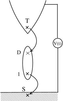
FIG. 1.: System : the molecule (quantum dot) sandwiched between a substrate and an STM tip.

Consider the model for a metal–molecule–metal junction depicted in Fig. 1. The substrate and the tip are assumed to be metallic and are both described by an infinite bandwidth model. Both are therefore characterized by constant density of states $\rho_{S}$ and $\rho_{T}$.

In turn, the molecule will consist either of a single dot or of a conjugated structure (described by a tight binding Hamiltonian). It contains sites numbered from $1$ to $D$. The connection between the molecule and the substrate occurs on site $1$, while the connection between the molecule and the tip is located at site $D$. This general approach allows to compute the transport properties for a molecule with an arbitrary number of sites, but specific plots will be obtained for $D=1$ and $D=2$.

To be more specific, the connection between the molecule and the substrate is assumed to be quite strong. Indeed, such strong binding to a substrate is known to occur when the molecule is functionalized: when for instance an end group of atoms in the molecule is replaced by a sulphur atom, which has strong binding properties on a gold substrate.

When the other electrode (the STM tip) is brought close to the molecule, and a bias voltage is imposed between both metallic electrodes, non equilibrium flow of electrons occurs. The key point of this work is to use an alternating current STM for probing transport. This is modeled by adding an alternating contribution to the DC bias $V_{0}$ imposed on the junction: $V(t)=V_{0}+V_{1}cos(\omega t)$ where $V_{1}$ is the amplitude of the AC bias voltage and $\omega$ is its frequency.

The sites involved in the junction between the molecule and the tip are denoted $D$ (as in dot) and $T$ (tip). With this convention, the Hamiltonian describing tunneling through this junction reads:

$$H_{TD}(t)=\Gamma(t)c^{\dagger}_{T}c_{D}+\Gamma^{*}(t)c^{\dagger}_{D}c_{T}$$ (1)

where $c/c^{\dagger}$ are fermionic annihilation/creation operators. The time dependence of the voltage bias is thus included in the hopping term using the Peierls substitution: starting from a formulation where the electric field at the junction is described solely by a scalar potential, a gauge transformation with gauge parameter $e\chi(t)c=-e\int V(t)dt$ is performed. The phase of the amplitude has a linear dependence associated with the DC bias, but it also contains a modulation due to the AC voltage:

$$\Gamma(t) = \Gamma^{0}_{T}\exp[-ie\chi(t)/c]$$ (2)

$$= \Gamma^{0}_{T}\exp(i\left(\omega_{0}t+\frac{\omega_{1}}{\omega}sin(\omega t)\right))$$ (3)

where $\Gamma^{0}_{T}$ is the time independent tunneling amplitude of the hopping between the tip and the molecule, and $\omega_{0,1}\equiv eV_{0,1}$.

An advantage of the Peierls substitution is that the current operator can be directly obtained by differentiating the hopping Hamiltonian with respect to the gauge parameter:

$$\hat{I}(t)=-c\frac{\partial H_{TD}(t)}{\partial\chi(t)}$$ (4)

Moreover, the current–current correlations (the current noise) are defined by

$$S(t,t^{\prime})={1\over 2}\left[\langle\hat{I}(t)\hat{I}(t^{\prime})+\hat{I}(t^{\prime})\hat{I}(t)\rangle-\langle\hat{I}(t)\rangle\langle\hat{I}(t^{\prime})\rangle\right]$$ (5)

Note that this correlator is symmetrized, which is appropriate when computing zero frequency noise: when considering the finite frequency spectral density of noise, this ceases to be true and one needs to consider the unsymmetrized correlator, which makes the difference between emission or absorption [22].

III Non-equilibrium transport

Note that because of the time dependent bias, any straightforward extension of the Landauer approach has to be ruled out, and the Keldysh formalism is employed.

The expectation value of the current (Eq. (4)) can be directly cast in terms of the spectral Green’s functions. For the noise (Eq. (5)), we can factorize the two body correlation function following a mean field decoupling scheme, which is exact for non-interacting electrons. Green’s functions are represented by $2\times 2$ matrices: each time argument can be pinned on either branch of the Keldysh time contour. However, recall that these Green’s functions are not independent. For convenience, here, one chooses to use the version of Dyson equations for advanced, retarded and spectral Green’s functions :

$$G^{a}_{\alpha\beta}(t,t^{\prime}) = i\,\Theta(t^{\prime}-t)\langle\{c_{\alpha}(t),c_{\beta}^{+}(t^{\prime})\}\rangle$$ (6)

$$G^{r}_{\alpha\beta}(t,t^{\prime}) = -i\,\Theta(t-t^{\prime})\langle\{c_{\alpha}(t),c_{\beta}^{+}(t^{\prime})\}\rangle$$ (7)

$$G^{+-}_{\alpha\beta}(t,t^{\prime}) = i\langle c^{\dagger}_{\beta}(t^{\prime})c_{\alpha}(t)\rangle$$ (8)

$$G^{-+}_{\alpha\beta}(t,t^{\prime}) = -i\langle c_{\alpha}(t)c^{\dagger}_{\beta}(t^{\prime})\rangle$$ (9)

Here $\alpha,\beta$ are terminal indices. Inserting these Green’s functions in the current and the real time current-current correlator yields:

$$I(t) = 2eRe\left[\Gamma(t)G^{+-}_{DT}(t,t)\right]$$ (10)

$$S(t,t^{\prime}) = 2e^{2}Re\Big{[}\Gamma(t)\Gamma^{*}(t^{\prime})G^{+-}_{TT}(t^{\prime},t)G^{-+}_{DD}(t,t^{\prime}))$$ (12)

$$~{}~{}~{}~{}~{}~{}~{}~{}+\Gamma^{*}(t)\Gamma(t^{\prime})G^{+-}_{DD}(t^{\prime},t)G^{-+}_{TT}(t,t^{\prime})\Big{]}$$

Here one is only interested in the lowest order contribution in the tip–molecule hopping amplitude. The Dyson equation for the above Green’s function reads (omitting terminal indices summations and time integrations):

$$G^{a,r} = g^{a,r}(1+\Sigma^{a,r}G^{a,r})$$ (13)

$$G^{+-,-+} = (1+G^{r}\Sigma^{r})g^{+-,-+}(1+\Sigma^{a}G^{a})$$ (14)

In the perturbative scheme, the $G$’s are the dressed Green’s functions -which have both diagonal and non-diagonal non-zero elements in the terminal indices- while the $g$’s are the bare Green’s functions with only diagonal non-vanishing elements. The self-energies $\Sigma$ are related to the hopping amplitude : $\Sigma^{r}=\Gamma(t)$, $\Sigma^{a}=\Gamma^{*}(t)$, $\Sigma^{+-,-+}=0$. At this point the time-dependent hopping amplitude is expanded using the generating function of the Bessel functions[30] $\Gamma(t)=\Gamma^{0}_{T}\sum_{n=-\infty}^{+\infty}\;e^{i(\omega_{0}+n\omega)t}J_{n}\left(\frac{\omega_{1}}{\omega}\right)$.

The strong coupling between the substrate and the molecule allows to define a compound molecule–substrate system. The Green’s function of the molecule becomes dressed by the substrate-molecule coupling, which can be treated non perturbatively. In the following, $\tilde{G}$ denotes the non-equilibrium dressed Green’s functions for this composite system.

A Fourier transform ($h(\omega)=\int_{-\infty}^{+\infty}dte^{i\omega t}h(t)$) helps to characterize the current response at finite frequency. Because time-translational invariance is broken by the AC bias, a double Fourier transform is implied for the noise:

$$I(\Omega) = e|\Gamma^{0}_{T}|^{2}\sum_{n,m}J_{n}\left({\omega_{1}\over\omega}\right)J_{m}\left({\omega_{1}\over\omega}\right)\int_{-\infty}^{+\infty}d\omega_{2}$$ (15)

$$\times\Big{\{} [\delta(\Omega+(n-m)\omega)+\delta(\Omega-(n-m)\omega)]$$ (17)

$$~{}~{}~{}~{}~{}~{}~{}~{}~{}~{}~{}~{}\times\tilde{G}^{+-}_{DD}(\omega_{2})g^{a}_{TT}(\omega_{2}-\omega_{0}-m\omega)$$

$$+ \delta(\Omega+(n-m)\omega)$$ (20)

$$\times\Big{[}\tilde{G}^{r}_{DD}(\omega_{2})g^{+-}_{TT}(\omega_{2}-\omega_{0}-m\omega)$$

$$~{}~{}~{}~{}~{}~{}-\tilde{G}^{a}_{DD}(\omega_{2})g^{+-}_{TT}(\omega_{2}-\omega_{0}-n\omega)\Big{]}\Big{\}}$$

$$S(\Omega,\Omega^{\prime}) = e^{2}|\Gamma^{0}_{T}|^{2}\sum_{n,m}J_{n}\left({\omega_{1}\over\omega}\right)J_{m}\left({\omega_{1}\over\omega}\right)$$ (22)

$$~{}~{}\times\delta(\Omega+\Omega^{\prime}+(n-m)\omega)\int_{-\infty}^{+\infty}d\omega_{2}$$

$$\times\Big{\{}\tilde{G}^{-+}_{DD}(\omega_{2}) \Big{[}g^{+-}_{TT}(\omega_{2}+\Omega^{\prime}-\omega_{0}-m\omega)$$ (24)

$$~{}~{}~{}~{}~{}~{}~{}+g^{+-}_{TT}(\omega_{2}-\Omega^{\prime}-\omega_{0}-n\omega)\Big{]}$$

$$+\tilde{G}^{+-}_{DD}(\omega_{2}) \Big{[}g^{-+}_{TT}(\omega_{2}+\Omega-\omega_{0}-m\omega)$$ (26)

$$~{}~{}~{}~{}~{}~{}~{}+g^{-+}_{TT}(\omega_{2}-\Omega-\omega_{0}-n\omega)\Big{]}\Big{\}}$$

At this point, it is convenient to introduce the tip’s Green’s functions (Appendix A 1) where $\rho_{T}$ is the density of states in the tip. The noise and the current thus become:

$$I(\Omega) = ie\pi\rho_{T}|\Gamma^{0}_{T}|^{2}\sum_{n,m}J_{n}\left({\omega_{1}\over\omega}\right)J_{m}\left({\omega_{1}\over\omega}\right)$$ (27)

$$\times\Big{\{} [\delta(\Omega+(n-m)\omega)+\delta(\Omega-(n-m)\omega)]$$ (29)

$$\times\int_{-\infty}^{+\infty}d\omega_{2}\tilde{G}^{+-}_{DD}(\omega_{2})$$

$$+2 \delta(\Omega+(n-m)\omega)$$ (32)

$$\times\Big{[}\int_{-\infty}^{\omega_{0}+m\omega}d\omega_{2}\left(\tilde{G}^{r}_{DD}(\omega_{2})-\tilde{G}^{a}_{DD}(\omega_{2})\right)$$

$$~{}~{}~{}~{}~{}~{}-\int_{\omega_{0}+m\omega}^{\omega_{0}+n\omega}d\omega_{2}\tilde{G}^{a}_{DD}(\omega_{2})\Big{]}\Big{\}}$$

$$S(\Omega,\Omega^{\prime}) = (2e)ie\pi\rho_{T}|\Gamma^{0}_{T}|^{2}\sum_{n,m}J_{n}\left({\omega_{1}\over\omega}\right)J_{m}\left({\omega_{1}\over\omega}\right)$$ (34)

$$\times\delta(\Omega+\Omega^{\prime}+(n-m)\omega)$$

$$\times\Big{\{} -2\int_{\omega_{0}+m\omega-\Omega}^{+\infty}d\omega_{2}\;\tilde{G}^{+-}_{DD}(\omega_{2})$$ (37)

$$+2\int_{-\infty}^{\omega_{0}+m\omega-\Omega}d\omega_{2}\tilde{G}^{-+}_{DD}(\omega_{2})$$

$$+\int_{\omega_{0}+m\omega-\Omega}^{\omega_{0}+n\omega+\Omega}d\omega_{2}\left[\tilde{G}^{-+}_{DD}(\omega_{2})+\tilde{G}^{+-}_{DD}(\omega_{2})\right]\Big{\}}$$

The noise and current are fully determined once the dressed Green’s functions of the molecule (dot) are specified. Note that Eqs. (32) and (LABEL:noise_dressed) are valid for an arbitrary model of the molecule/substrate, which could in principle include interactions. The $\delta$ functions in Eq. (32) and (LABEL:noise_dressed) restrict the frequency dependance of the current to integer multiple of the driving frequency $\omega$. The mth harmonic of the current, $I(m\omega)$, is obtained by integrating Eq. (32) on the detector resolution $s$ : $I(m\omega)=\int_{m\omega-s/2}^{m\omega+s/2}d\Omega I(\Omega)$, then getting rid of the $\delta$ function singularities. The detector resolution $s$ is of course much smaller than all the frequencies of this problem.

Here we focus on a single dot and on a two site molecule. The dressed Green’s functions are derived in Appendices B 1 and B 2. For the single dot they read:

$$\tilde{G}^{a,r}_{DD}(\Omega) = \frac{1}{\Omega-E_{D}\mp i\pi\rho_{S}\Gamma_{S}^{2}}$$ (39)

$$\tilde{G}^{+-}_{DD}(\Omega) = 2i\pi\rho_{S}\Gamma_{S}^{2}\frac{f(\Omega-E_{F})}{(\Omega-E_{D})^{2}+(\pi\rho_{S}\Gamma_{S}^{2})^{2}}$$ (40)

$$\tilde{G}^{-+}_{DD}(\Omega) = -2i\pi\rho_{S}\Gamma_{S}^{2}\frac{(1-f(\Omega-E_{F}))}{(\Omega-E_{D})^{2}+(\pi\rho_{S}\Gamma_{S}^{2})^{2}}$$ (41)

The coupling to the metallic substrate imposes a width $\pi\Gamma_{S}^{2}\rho_{S}$. Furthermore, the occupation of the dot (as it appears in $\tilde{G}^{+-}_{DD}$) is specified by the Fermi function $f$ of the substrate.

For two site molecule, the dressed Green’s functions are derived in Appendix B 2 :

$$\tilde{G}^{a,r}_{DD}(\Omega) = -\frac{\Omega-i\pi\rho_{S}\Gamma_{S}^{2}}{t^{2}-\Omega(\Omega-i\pi\rho_{S}\Gamma_{S}^{2})}$$ (43)

$$\tilde{G}^{+-}_{DD}(\Omega) = 2i\pi\rho_{S}\Gamma_{S}^{2}\frac{t^{2}f(\Omega-E_{F})}{|t^{2}-\Omega(\Omega+i\pi\rho_{S}\Gamma_{S}^{2})|^{2}}$$ (44)

$$\tilde{G}^{-+}_{DD}(\Omega) = -2i\pi\rho_{S}\Gamma_{S}^{2}\frac{t^{2}[1-f(\Omega-E_{F})]}{|t^{2}-\Omega(\Omega+i\pi\rho_{S}\Gamma_{S}^{2})|^{2}}$$ (45)

where $t$ is the hopping between the two sites of the molecule.

Note that, in both cases (single dot/ double dot), the spectral dressed Green functions may be written in terms of the density of states of the dressed system :

$$\tilde{G}^{+-}_{DD}(\Omega) = 2iIm[\tilde{G}^{a}_{DD}(\Omega)]f(\Omega-E_{F})$$ (46)

$$\tilde{G}^{-+}_{DD}(\Omega) = -2iIm[\tilde{G}^{a}_{DD}(\Omega)][1-f(\Omega-E_{F})]$$ (47)

where $Im[\tilde{G}^{a}_{DD}(\Omega)]/\pi$ is the density of states on site $D$ . This density should be computed directly from the expression of the advanced dressed Green’s function :

$$Im[\tilde{G}^{a}_{DD}(\Omega)]|_{1dot} = \frac{\pi\rho_{S}\Gamma_{S}^{2}}{(\Omega-E_{D})^{2}+(\pi\rho_{S}\Gamma_{S}^{2})^{2}}$$ (49)

$$Im[\tilde{G}^{a}_{DD}(\Omega)]|_{2dots} = \frac{\pi\rho_{S}\Gamma_{S}^{2}t^{2}}{(t^{2}-\Omega^{2})^{2}+(\pi\rho_{S}\Gamma_{S}^{2})^{2}\Omega^{2}}$$ (50)

In the following, the integrated version of the density of states denoted by $F$ is needed :

$$F(a,b)=\int_{a}^{b}du\;Im[\tilde{G}^{a}_{DD}(u)]~{}.$$ (51)

IV Photo-assisted shot noise

One is now in a position to compute the current harmonics and the photo-assisted shot noise using the explicit expressions for the dressed Green’s functions. Before displaying these results, as a reference it is useful to recall what happens in a tunnel junction between two metallic electrodes (no molecule). This allows to relate to the results of Ref. [31], where photo-assisted shot noise was studied in a mesoscopic conductor from the point of view of scattering theory. For the current and the noise our perturbation scheme yields at zero frequencies :

$$I(\Omega=0) = 4e\pi^{2}\rho_{T}\rho_{S}\Gamma_{S}^{2}\sum_{n}J_{n}^{2}\left({\omega_{1}\over\omega}\right)(\omega_{0}+n\omega-E_{F})$$ (52)

$$S(0,0) = (2e)4e\pi^{2}\rho_{T}\rho_{S}\Gamma_{S}^{2}\sum_{n}J_{n}^{2}\left({\omega_{1}\over\omega}\right)|\omega_{0}+n\omega-E_{F}|$$ (53)

The noise is continuous, but its derivative has jumps at integer values of $\omega_{0}/\omega$, precisely the result of Ref. [31] when one assumes that the transmission coefficient used for scattering theory does not depend on energy. It is therefore relevant to generalize these results to a situation where the “mesoscopic system” has an internal discrete level structure, which is the case for molecular electronic transport. This is expected to have repercussions on both the current harmonics and the noise.

Using the general formulation of the spectral Green’s functions (Eq. 46), the zero frequencies noise read :

$$S(0,0) = 8e^{2}\pi\rho_{T}|\Gamma^{0}_{T}|^{2}\sum_{n}\bigg{[}J_{n}^{2}\left({\omega_{1}\over\omega}\right)sgn(\omega_{0}+n\omega-E_{F})$$ (56)

$$~{}\times F(E_{F},\omega_{0}+n\omega)\bigg{]}$$

where $F(a,b)$ is defined in Eq. (51).

In order to make a diagnosis on the spectrum, it is useful to display also the first derivative of the noise with respect to the DC voltage:

$$\frac{dS(0,0)}{d\omega_{0}} = 8e^{2}\pi\rho_{T}|\Gamma^{0}_{T}|^{2}\sum_{n}\bigg{[}J_{n}^{2}\left({\omega_{1}\over\omega}\right)sgn(\omega_{0}+n\omega-E_{F})$$ (58)

$$~{}\times Im[\tilde{G}^{a}_{DD}(\omega_{0}+n\omega)]\bigg{]}$$

A Single dot problem

One of the motivations for studying photo-assisted shot noise is to probe the finite frequency spectral density of noise using the external frequency $\omega$ of the AC bias. We will therefore focus on the photo-assisted shot noise with both frequencies in Eq. (LABEL:noise_dressed) set to zero, because low frequency measurements (still above, say $100KHz$, to avoid $1/f$ noise) are more accessible experimentally than high frequency ones. Using the definition of the density of states for a single dot system (Eq. (49)) and after performing the integration over frequencies in Eqs. (56) and (58), the noise at zero frequencies and its derivative read:

$$S(0,0)=8e^{2}\pi\rho_{T}|\Gamma^{0}_{T}|^{2}\sum_{n}J_{n}^{2}\left({\omega_{1}\over\omega}\right)sgn(\omega_{0}+n\omega-E_{F})$$ (60)

$$\times\left[\arctan\left({(E_{D}-E_{F})\over\pi\rho_{S}\Gamma_{S}^{2}}\right)-\arctan\left({(E_{D}-\omega_{0}-n\omega)\over\pi\rho_{S}\Gamma_{S}^{2}}\right)\right]$$ (61)

(62)

$$\frac{dS(0,0)}{d\omega_{0}} = 8e^{2}\pi^{2}\rho_{T}\rho_{S}\Gamma_{S}^{2}|\Gamma^{0}_{T}|^{2}\sum_{n}J_{n}^{2}\left({\omega_{1}\over\omega}\right)$$ (64)

$$~{}\times\frac{sgn(\omega_{0}+n\omega-E_{F})}{(\omega_{0}+n\omega-E_{D})^{2}+(\pi\rho_{S}\Gamma_{S}^{2})^{2}}$$

\psfrag{s00}{$S(0,0)$}\psfrag{ds00tototttttttttt}{${dS(0,0)}/{d\omega_{0}}$}\psfrag{omega0}{${\omega_{0}}/{\omega}$}\psfrag{2electrodesgggggg}{2 electrodes}\psfrag{gs0.1}{$\Gamma_{S}=0.1$}\psfrag{gs1.0}{$\Gamma_{S}=1.0$}\psfrag{gs10}{$\Gamma_{S}=10.$}\psfrag{ef}{$E_{F}$}\includegraphics[width=227.62204pt]{petitacter.eps}

FIG. 2.: Zero–frequencies noise $S(0,0)$ (upper graph) and its first derivative $dS(0,0)/d\omega_{0}$ (lower graph) as a function of the ratio $\omega_{0}/\omega$ in the regime of a small AC bias ($\omega_{1}/\omega=0.1$) for the single dot system. Fermi energy of the substrate $E_{F}$ is fixed to $-1.4\omega$ and energy level of the dot $E_{D}$ is the origin of the energy. Comparisons are made between the two electrodes case and different values of hopping $\Gamma_{S}$ in the dot–metal junction.

The quantities which are plotted on Figs 2 to 6 are normalized according to the prefactors which appear on Eqs. (62) and (64).

Consider first the case where the dot level lies above the Fermi level of the substrate. Fig. 2 displays the noise and its first derivative with respect to the DC bias for a small value of the AC bias amplitude. From the point of view of our analytical results, this means that very few terms contribute to the sum over integers in Eq. (62): $n=0$ dominates. In the case of large broadening, we recover similar results to the two electrodes system. The dot is metallized to the extent that transport is fully specified by the two Fermi distributions of the electrodes. As the broadening decreases, the noise acquires a step-like structure close to the bare dot level, which gets sharper for lower $\Gamma_{S}$. This is associated to the fact that the current increases drastically at this particular DC bias. Far from this DC bias value, the noise saturates because the AC bias does not allow for the exchange of “photon” quanta $\omega$. The peak appearing in the derivative of the noise for the case of a two electrodes system is a consequence of the abrupt change of sign of the current.

\psfrag{s00}{$S(0,0)$}\psfrag{ds00tototttttttttt}{${dS(0,0)}/{d\omega_{0}}$}\psfrag{omega0}{${\omega_{0}}/{\omega}$}\psfrag{2electrodes}{2 electrodes}\psfrag{gs0.1}{$\Gamma_{S}=0.1$}\psfrag{gs1.0}{$\Gamma_{S}=1.0$}\psfrag{gs10}{$\Gamma_{S}=10.$}\psfrag{ef}{$E_{F}$}\includegraphics[width=227.62204pt]{moyenacbis.eps}

FIG. 3.: Same as Fig.2 for an AC bias: $\omega_{1}/\omega=1.0$.

When one further increases the AC bias (Fig. 3), photonic exchanges become relevant: this is illustrated by the appearance of new shoulders in the noise (peaks in the noise derivative) for integer values of the ratio $\omega_{0}/\omega$. The dominant peak in the derivative is located at the dot level $\omega_{0}=0$. Side peaks at $\omega_{0}=\pm\omega$ are clearly visible, while those at $\omega_{0}=\pm 2\omega$ can only be identified with the help of the noise derivative. These peaks are smoothed when the substrate coupling is increased, eventually leading to metallization as before.

\psfrag{s00}{$S(0,0)$}\psfrag{ds00tototttttttttt}{${dS(0,0)}/{d\omega_{0}}$}\psfrag{omega0}{${\omega_{0}}/{\omega}$}\psfrag{2electrodes}{2 electrodes}\psfrag{gs0.1}{$\Gamma_{S}=0.1$}\psfrag{gs1.0}{$\Gamma_{S}=1.0$}\psfrag{gs10}{$\Gamma_{S}=10.$}\psfrag{ef}{$E_{F}$}\includegraphics[width=227.62204pt]{grandacbis.eps}

FIG. 4.: Same as Fig.2 for an AC bias: $\omega_{1}/\omega=10.0$.

Turning now to the case of a large AC bias (Fig. 4), one notices that the step like structure is preserved but the width of the steps is apparently doubled compared to Fig. 3. This is only apparent, as the noise derivative displays secondary peaks associated with odd photon absorption/emission. The relative importance of odd and even photon peaks can be traced to a high sensitivity of the noise with respect to the AC bias amplitude $\omega_{1}$, due to the oscillations of the Bessel functions (see Eq. (64)).

\psfrag{s00}{$S(0,0)$}\psfrag{ds00}{${dS(0,0)}/{d\omega_{0}}$}\psfrag{ds00tototttttttttt}{${dS(0,0)}/{d\omega_{0}}$}\psfrag{omega0}{${\omega_{0}}/{\omega}$}\psfrag{2electrodes}{2 electrodes}\psfrag{gs0.1}{$\Gamma_{S}=0.1$}\psfrag{gs1.0}{$\Gamma_{S}=1.0$}\psfrag{gs10}{$\Gamma_{S}=10.$}\psfrag{ef}{$E_{F}$}\includegraphics[width=227.62204pt]{moyenacresbis.eps}

FIG. 5.: Same as Fig.3 in the case of a resonance between the energy level of the dot and the Fermi energy of the substrate: $E_{F}=E_{D}=0$.

The behavior of this system turns out to be strongly dependent on the location of the dot level. In Fig. 5, the dot level matches the Fermi level of the substrate. The AC bias amplitude has been adjusted as in Fig. 3 where essentially $\omega_{0}=0,\pm\omega$ give salliant features. First, notice that the noise does not display steps any more. Qualitatively, it is understood that current flows when the absolute value of the bias is large compared to the the “photon energy” $\omega$: in this situation there is no balance between carriers emmitted from the tip to the substrate, and vice versa. Next, the current – and thus the noise – must vanish when the tip and the substrate have matching Fermi energies. More interesting is the reduction of the noise observed when $\omega_{0}=\pm\omega$. Current can flow with the help of virtual transitions through the dot, but for this AC bias where essentially only single photon transitions contribute, there is an additional channel which brings about noise reduction. This explains the two side dips in the noise at $\omega_{0}=\pm\omega$ in Fig. 5. It is interesting to note that the behavior of the noise and of its derivative is drastically modified only when the coupling to the substrate is small, whereas for a metallized dot the typical behavior associated with two metallic electrodes is recovered.

B Two–site molecule

The expressions for the dressed Green’s functions of the two–site molecule are inserted in the expressions for the zero–frequencies noise. The two–site molecule has a hopping amplitude $t$ between the two sites, so the bonding and anti-bonding orbitals are separated by $2t$. Note that when the Fermi level of both the tip and the substrate lie between these orbitals, these two level can mimic the HOMO (Highest Occupied Molecular Orbital) and the LUMO (Lowest Unoccupied Molecular Orbital) of a more complex molecule. Here one is interested in understanding how the presence of the two sites modifies the noise with respect to the single dot case. Expressions for the noise and its derivative are given in Eqs. (56) and (58) with the corresponding density of states (see Eq. (49)).

\psfrag{S00}{$S(0,0)$}\psfrag{omega0}{${\omega_{0}}/{\omega}$}\psfrag{a/}{a)}\psfrag{b/}{b)}\includegraphics[width=227.62204pt]{s002dot.eps}

FIG. 6.: Zero–frequencies noise $S(0,0)$ for a two–site molecule as a function of the ratio $\omega_{0}/\omega$ for AC bias $\omega_{1}/\omega=5.0$. Full line , $\Gamma_{S}=0.001$; dashed line, $\Gamma_{S}=1.0$; dashed-dotted, $\Gamma_{S}=3.0$; dotted line, $\Gamma_{S}=100$. The hopping between the two sites is $t=3\omega$. Vertical dashed line correspond to the bonding and antibonding orbitals. Plots are given for: a) $E_{F}=-1.4\omega$; b) $E_{F}=t$ (resonance with highest level)

Consider first the case where the Fermi level of the substrate is located in between the two molecular levels (top part of Fig. 6). For sharp levels (small coupling to the substrate), the noise has a staircase structure, as expected from photo-assisted transport, but contrary to the single dot case, the steps are not monotonous. The noise has minima close to the location of the bonding and antibonding orbitals. When the levels are broadened by a better coupling to the substrate, these steps are smoothed out, but the minima survive at first. Further increasing the coupling to the substrates gives rises to monotonous steps which resemble the noise characteristic of a single dot with a sharp level. This can be explained as follows. As long as the substrate coupling $\Gamma_{S}$ is smaller than the hopping between the two sites of the molecule, increasing $\Gamma_{S}$ smoothes out the photo–assisted shot noise. But for $\Gamma_{S}>t$, the system behaves as if it was a single dot (the dot closest to the tip). This interpretation is confirmed by comparing the density of states of the double dots/single dot case (Eq. (49)) : the limit of a very large broadening $\Gamma_{S}>>t$ for the double dots density of states is simply the single dot density of states with a width $t^{2}/(\pi\rho_{S}\Gamma_{S}^{2})(<<1)$. Therefore, increasing $\Gamma_{S}$ brings sharper features in the noise rather than smoothing them. Then, the noise associated with the large coupling in Fig. 6, is quite similar to the staircase encountered in Fig. 4.

Turning now to the situation where the Fermi level of the substrate coincides with the highest orbital of the molecule, one notices a noise characteristic which is again similar to a single dot level, except for the fact that it is inverted. For weak coupling to the substrate, one gets sharp steps, but as these steps are smoothed upon increasing the coupling, one recovers the same crossover back to the sharp steps of a single level. It does seem natural that if it is now the lowest level of the molecule which is pinned to the substrate Fermi energy, the noise characteristic is inverted with respect to Fig. 6b (not shown). In particular, for a very strong substrate coupling, we recover curves similar to Fig. 3.

V Higher harmonics of the current

Using the definition of the density of states in Eq. (49), Eq. (32) gives for the mth harmonics of the current :

$$I(\Omega=m\omega)=2e\pi\rho_{T}|\Gamma^{0}_{T}|^{2}\sum_{n}J_{n}\left({\omega_{1}\over\omega}\right)\\ \times\Bigg{\{}J_{n+m}\left({\omega_{1}\over\omega}\right)(F(-\infty,\omega_{0}+(n+m)\omega)+F(E_{F},\omega_{0}+n\omega))\\ -J_{n-m}\left({\omega_{1}\over\omega}\right)F(-\infty,E_{F})\Bigg{\}}\\$$ (65)

The stationary current is given by taking $m=0$ in this expression :

$$I(\Omega=0)=4e\pi\rho_{T}|\Gamma^{0}_{T}|^{2}\sum_{n}J_{n}^{2}\left({\omega_{1}\over\omega}\right)F(E_{F},\omega_{0}+n\omega)$$ (66)

According to Eq. (56), Shottky relation occurs between the zero frequencies noise and the stationary current : $S(0,0)=2e|I(\Omega=0)|$.

The density of states for the one/double dots sytem is even (Eq. (49)) so, according to Eq. (65), the harmonics of the current have symmetry properties : $I(\omega)$ and $I(3\omega)$ are even and $I(2\omega)$ is odd.

The harmonics of the current plotted in Figs 7 and 8 are normalized by $2e\pi\rho_{T}|\Gamma^{0}_{T}|^{2}$.

A Single dot problem

The behavior of the finite frequency higher harmonics of the current $I(m\omega)$ is examined where $\omega$ is the driving frequency of the AC-field.

The stationary current is computed from Eq. (66) :

$$I(\Omega=0)=4e\pi\rho_{T}|\Gamma^{0}_{T}|^{2}\sum_{n}J_{n}^{2}\left({\omega_{1}\over\omega}\right)$$ (68)

$$~{}\left[\arctan\left({(E_{D}-E_{F})\over\pi\rho_{S}\Gamma_{S}^{2}}\right)-\arctan\left({(E_{D}-\omega_{0}-n\omega)\over\pi\rho_{S}\Gamma_{S}^{2}}\right)\right]$$ (69)

Fig. 7 shows the zero-frequency component and the first three harmonics as a function of the ratio $\omega_{0}/\omega$ for different values of the substrate-molecule coupling which defines the effective width of the single energy level of dot, $\pi\rho_{S}\Gamma_{S}^{2}$. The zeroth harmonic represents a generalized Current-Voltage, I-V, curve. For a dot with a sharp level structure, the I-V curve displays a staircase structure with steps width corresponding to either $\Delta\omega_{0}=\omega$ or $\Delta\omega_{0}=2\omega$ associated with photo-assisted transport. Depending on the overlap between the Fermi distribution of the substrate and the band-width of the impurity the zeroth frequency harmonic can be either positive or negative leading to current inversion at large negative DC bias. The Ohmic regime is recovered for large $\Gamma_{S}$ which corresponds to the physical limit of a metal (See inset on Fig. 7a).

A general feature of the higher harmonics is the presence of maxima and minima whose number increases with the order of the harmonic. These oscillations are damped as $\Gamma_{S}$ increases and the higher order responses vanish while the zeroth harmonic survives. This has important implications for the experiment suggested in reference [20], because large $\Gamma_{S}$ mimics in our model a metallized dot, precisely the situation where Kochanski suggested there would be no higher-order signal. This also agrees with the results on insulating surfaces and stresses the importance of exploring the use of higher harmonics for more general molecule-electrode interfaces.

\psfrag{omega0}{${\omega_{0}}/{\omega}$}\psfrag{H0}{$I(0)$}\psfrag{H1}{$I(\omega)$}\psfrag{H2}{$I(2\omega)$}\psfrag{H3}{$I(3\omega)$}\includegraphics[width=170.71652pt]{1dot_harms_ok.eps}

FIG. 7.: Stationary current and its three lowest harmonics as a function of the ratio $\omega_{0}/\omega$ for the single dot system. The AC bias is fixed to $\omega_{1}=5.0\omega$. The Fermi energy and the dot level are the same than in previous graph ($E_{F}=-1.4\omega$, $E_{2}=0.0$). Full line, $\Gamma_{S}=0.001$; dashed line, $\Gamma_{S}=1.0$; dashed-dotted, $\Gamma_{S}=3.0$; dotted line, $\Gamma_{S}=1000.0$. Inset : stationary current as a function of $\omega_{0}/\omega$ for small values of this ratio ($\Gamma_{S}=1000.0$).

B Two–site molecule

The double dots current harmonics are obtained from Eq. (65) using the appropriate $F$ function (see Eqs. (49) and (51))

Turning now to the discussion of the current harmonics for the 2 dot system (Fig. 8), one first notices -as observed in the single dot case- that higher order harmonics oscillate more. For comparison with the previous case, the 2 dot levels have been chosen symmetrically around the position of the single dot level in Fig. 7.

Starting with sharp levels (poor coupling to the substrate), the zeroth harmonics has a monotonous staircase structure, ranging from negative to positive value. The first harmonic is positive, as in the one dot case, and has a broader width due to the spacing between the two levels. For the next two harmonics, the oscillatory behaviour is more prononced than in the one dot case. As in the single dot case, the harmonics have symmetry properties : $I(\omega)$ is even, $I(2\omega)$ is odd, $I(3\omega)$ is even.

Upon increasing the levels widths, the amplitude of the oscillations first decreases (up to $\Gamma_{S}\sim t$). For very large coupling (dotted curve on the figure), we recover exactly the one dot case : as explained before, for large $\Gamma_{S}$, the density of states of the double site molecule (Eq. (49)) corresponds to the density of states in the single dot case for a very small broadening $t^{2}/(\pi\rho_{S}\Gamma_{S}^{2})$.

\psfrag{omega0}{${\omega_{0}}/{\omega}$}\psfrag{H0}{$I(0)$}\psfrag{H1}{$I(\omega)$}\psfrag{H2}{$I(2\omega)$}\psfrag{H3}{$I(3\omega)$}\includegraphics[width=170.71652pt]{2dot_harms_ok.eps}

FIG. 8.: Stationary current and its three lowest harmonics as a function of the ratio $\omega_{0}/\omega$ for the two site molecule. The alternative voltage is fixed to $\omega_{1}=5.0\omega$. The Fermi energy $E_{F}=-1.4\omega$ and $t=3.0$. Full line, $\Gamma_{S}=0.001$; dashed line, $\Gamma_{S}=1.0$; dashed-dotted, $\Gamma_{S}=3.0$; dotted line, $\Gamma_{S}=1000.0$.

VI Conclusions

In this paper, we have studied the photo-assisted shot noise for a simple model of metal-molecule substrate junction which could prove to be relevant in alternating current STM experiment. The Keldysh method allowed to treat the time-dependent response of this system and in particular to express the noise in terms of the dressed Green’s functions of the molecule plus substrate compound. Contrary to scattering formulations of transport, the Keldysh approach allows to take into account the molecule occupancy correctly. While the present deals with non-interacting electrons throughout, the general approach allows to tackle more complicated systems where the molecule would include electron-electron interactions as they occur in carbon nanotubes or more complex nano-objects.

So far, the work on photo-assisted shot noise has focused mostly on mesoscopics conductors where the effective transmission coefficient has little energy level structure[32]. One of the purpose of this work was precisely to go beyond this limitation. In fact, we have seen that the presence of the molecule levels modifies drastically the staircase which is observed in the noise derivative as a function of bias. As the coupling to the substrate is increased, the sharp features which we observed get more pronounced.

This corresponds to a poorly conducting system (insulator). It is relevant to follow Kochansky’s intuition when analyzing the behaviour of the current harmonics as a function of this coupling. Indeed, the harmonics stay sharp in the case of an insulator. To our knowledge, this is the first time that this is addressed in a quantitative manner, albeit with the help of a simple model. The fact that the $I(3\omega)$ signal has been measured for insulating surfaces makes it reasonable to assume that the experiment with electrode-molecule junctions will soon be done. It is on this situation that the predictions of this model may be more relevant.

Future directions of research could include a time-dependent, self-consistent treatment of Coulomb interactions in the molecule. Electronic correlations has recently been addressed in References [17, 33, 34]. Another possible extension would be to describe the molecule using ab initio method, as used in [35, 36, 37] where the effect of an AC bias in molecular transport is also addressed.

A Unperturbed Green’s functions

1 For two electrodes

The non–equilibrium Green’s functions for a site $M$ ($M=T,S$) into a normal metal electrode are:

$$g^{+-}_{MM}(\Omega) = 2i\pi\rho_{M}f(\Omega)$$ (A1)

$$g^{-+}_{MM}(\Omega) = -2i\pi\rho_{M}[1-f(\Omega)]$$ (A2)

$$g^{a}_{MM}(\Omega) = i\pi\rho_{M}=g^{r*}_{MM}(\Omega)$$ (A3)

where $f(\Omega)$ is the Fermi distribution and $\rho_{M}$ is the local density of states on site $M$ near the Fermi level.

2 For one dot

Using the definitions of Keldysh Green’s functions in terms of creation/annihilation operators of electrons in the dot, we find the temporal (homogeneous) non–equilibrium Green’s functions:

$$g^{+-}_{DD}(\tau) = in^{0}_{D}e^{-iE_{D}\tau}$$ (A4)

$$g^{-+}_{DD}(\tau) = -i(1-n^{0}_{D})e^{-iE_{D}\tau}$$ (A5)

$$g^{a}_{DD}(\tau) = i\Theta(-\tau)e^{-iE_{D}\tau}$$ (A6)

$$g^{r}_{DD}(\tau) = -i\Theta(\tau)e^{-iE_{D}\tau}$$ (A7)

where $n^{0}_{D}$ is the number electron in the dot at time $0$, $E_{D}$ is the energy and $\Theta(t)$ is the Heaviside function .

Using a Fourier transform, the expressions of the Green’s functions in the frequency space look:

$$g^{+-}_{DD}(\Omega) = 2in^{0}_{D}\frac{\eta}{(\Omega-E_{D})^{2}+\eta^{2}}$$ (A9)

$$g^{-+}_{DD}(\Omega) = -2i(1-n^{0}_{D})\frac{\eta}{(\Omega-E_{D})^{2}+\eta^{2}}$$ (A10)

$$g^{a}_{DD}(\Omega) = \frac{1}{\Omega-E_{D}-i\eta}$$ (A11)

$$g^{r}_{DD}(\Omega) = \frac{1}{\Omega-E_{D}+i\eta}$$ (A12)

where $\eta$ is an infinitesimal positive constant.

3 For a linear system of $D$ dots ($D>1$)

A linear chain of $D$ dots is considered. The sites are labelled by $j=1..D$. The real hopping between two nearest neighbor sites is $t$. In such a system, eigen-energies and eigenfunctions of the site $j$ are given by:

$$\left\{\begin{array}[]{cc}E_{j}&=-2t\cos\left({\pi j\over D+1}\right)\\ \Psi_{j}(l)&=K_{j}\sin\left({\pi jl\over D+1}\right)\end{array}\right.$$ (A16)

where $j,l=1..D$. Eigenfunctions are normalized with $K_{j}$ given by:

$$|K_{j}|^{2}=\left[\sum_{l=1}^{D}\sin^{2}\left({\pi jl\over D+1}\right)\right]^{-1}$$ (A17)

The non–equilibrium Green’s functions can be derived using the previous expressions. In position and energy space, that yields:

$$g^{a}(l_{1},l_{2},E) = \sum_{n=1}^{D}|K_{n}|^{2}\frac{\sin\left({\pi nl_{1}\over D+1}\right)\sin\left({\pi nl_{2}\over D+1}\right)}{E+2t\cos\left({\pi n\over D+1}\right)-i\eta}$$ (A18)

$$g^{+-}(l_{1},l_{2},E) = 2i\pi\sum_{n=1}^{D}|K_{n}|^{2}\sin\left({\pi nl_{1}\over D+1}\right)\sin\left({\pi nl_{2}\over D+1}\right)$$ (A20)

$$~{}~{}~{}~{}~{}~{}~{}~{}~{}~{}\times\chi(E_{n})\delta(E-E_{n})$$

where $\chi(E)$ is the occupation number of energy level $E$ ($0$ or $1$) and $\eta$ is an infinitesimal positive constant. The retarded Green’s function is the complex conjugate of the advanced one. The $-+$ Green’s function is obtained by replacing $\chi(E_{n})$ by $-(1-\chi(E_{n}))$ in the $+-$ expression.

In this proposal, only the case $D=2$ is studied. The expressions of the normalization constants are $|K_{1}|^{2}=|K_{2}|^{2}=2/3$. The eigenfunctions and eigenvalues for each dot are given by:

$$\left\{\begin{array}[]{cc}E_{1}=-t&\;\;\;\;\;\;E_{2}=t\\ \Psi_{1}(l)=\sqrt{2\over 3}\sin\left({\pi l\over 3}\right)&\;\;\;\;\;\;\Psi_{2}(l)=\sqrt{2\over 3}\sin\left({2\pi l\over 3}\right)\end{array}\right.$$ (A23)

Introducing these expressions in (A18) yields:

$$g^{a}_{l_{1},l_{2}}(E) = {2\over 3}\left[{\sin\left({\pi l_{1}\over 3}\right)\sin\left({\pi l_{2}\over 3}\right)\over E+t-i\eta}+{\sin\left({2\pi l_{1}\over 3}\right)\sin\left({2\pi l_{2}\over 3}\right)\over E-t-i\eta}\right]$$ (A24)

$$g^{+-}_{l_{1},l_{2}}(E) = {4i\pi\over 3}\Big{[}\sin\left({\pi l_{1}\over 3}\right)\sin\left({\pi l_{2}\over 3}\right)\chi(-t)\delta(E+t)$$ (A26)

$$~{}~{}~{}~{}+\sin\left({2\pi l_{1}\over 3}\right)\sin\left({2\pi l_{2}\over 3}\right)\chi(t)\delta(E-t)\Big{]}$$

For the two dots system, only the Green’s functions for $l_{1},l_{2}=1,2$ are needed:

$$g^{a}_{11}(E) = g^{a}_{22}(E)={1\over 2}\left[{1\over E+t-i\eta}+{1\over E-t-i\eta}\right]$$ (A27)

$$g^{a}_{12}(E) = g^{a}_{21}(E)={1\over 2}\left[{1\over E+t-i\eta}-{1\over E-t-i\eta}\right]$$ (A28)

$$g^{+-}_{11}(E) = g^{+-}_{22}(E)=i\pi\left[\chi(-t)\delta(E+t)+\chi(t)\delta(E-t)\right]$$ (A29)

$$g^{+-}_{12}(E) = g^{+-}_{21}(E)=i\pi\left[\chi(-t)\delta(E+t)-\chi(t)\delta(E-t)\right]$$ (A30)

B Dressed Green’s functions

In this section, dressed Green’s functions that enter in the expression of the current and noise are derived. In the general case of a linear chain of $N$ dots, it is possible to compute the dressed Green’s functions using a linear set of Dyson equations. As explained in the previous section, the usual scheme is to isolate the sub–system composed by the substrate and the chain and then to express the dressed Green’s functions of the point contacts in term of the unperturbed Green’s functions of the isolated chain and of the substrate. Standard unperturbed Green’s functions of a metallic electrode are used for the substrate (Appendix A 1) including the Fermi energy $E_{F}$ and the density of states $\rho_{S}$ of the substrate.

1 For one dot

Here, only the system composed by the substrate ($S$) and one dot is considered. The hopping between the substrate and the molecule will be denoted by $\Gamma_{S}$ and will be chosen to be real. The dressed Green’s functions have homogeneity in time due to the time independence of the hopping Hamiltonian. It also permits to use directly the Dyson equation in frequency.

For the advanced and retarded Green’s function, using two Dyson equations rises:

$$\tilde{G}^{a,r}_{DD}(\Omega) = g^{a,r}_{DD}(\Omega)+g^{a,r}_{DD}(\Omega)\Sigma^{a,r}_{DS}\tilde{G}^{a,r}_{SD}(\Omega)$$ (B1)

$$= \frac{g^{a,r}_{DD}(\Omega)}{1\mp i\pi\rho_{S}\Gamma_{S}^{2}g^{a,r}_{DD}(\Omega)}$$ (B2)

where $\Sigma^{a,r}_{DS}=\Gamma_{S}$ the self energy associated to the hopping between the substrate and the dot and the upper/downer sign stands for the advanced/retarded Green’s functions. Little $g$ denote the unperturbed non–equilibrium Green’s functions for an isolated dot. Their expressions are given in Appendix A 2. Introducing these expressions in the dressed Green’s function of the point contact gives:

$$\tilde{G}^{a,r}_{DD}(\Omega) = \frac{1}{\Omega-E_{D}\mp i(\eta+\pi\rho_{S}\Gamma_{S}^{2})}$$ (B3)

where $\eta$ is an infinitesimal positive constant. This expression show the effect of the substrate. Due to the hopping $\Gamma_{S}$ between the dot and the electrode, a broadening of the energy level of the dot appears.

The limit when $\eta$ tends to $0$ is straightforward because these Green’s functions have no real poles:

$$\tilde{G}^{a,r}_{DD}(\Omega) = \frac{1}{\Omega-E_{D}\mp i\pi\rho_{S}\Gamma_{S}^{2}}$$ (B4)

The same technique allows to obtain the spectral dressed Green’s functions non–perturbatively:

$$\tilde{G}^{+-}_{DD}(\Omega) = \frac{g^{+-}_{DD}(\Omega)+2i\pi\rho_{S}\Gamma_{S}^{2}|g^{a}_{DD}(\Omega)|^{2}f(\Omega-E_{F})}{|1-i\pi\rho_{S}\Gamma_{S}^{2}g^{a}_{DD}(\Omega)|^{2}}$$ (B5)

$$\tilde{G}^{-+}_{DD}(\Omega) = \frac{g^{-+}_{DD}(\Omega)+2i\pi\rho_{S}\Gamma_{S}^{2}|g^{a}_{DD}(\Omega)|^{2}(1-f(\Omega-E_{F}))}{|1-i\pi\rho_{S}\Gamma_{S}^{2}g^{a}_{DD}(\Omega)|^{2}}$$ (B6)

Taking the limit when $\eta\rightarrow 0$ gives:

$$\tilde{G}^{+-}_{DD}(\Omega) = 2i\pi\rho_{S}\Gamma_{S}^{2}\frac{f(\Omega-E_{F})}{(\Omega-E_{D})^{2}+(\pi\rho_{S}\Gamma_{S}^{2})^{2}}$$ (B8)

$$\tilde{G}^{-+}_{DD}(\Omega) = -2i\pi\rho_{S}\Gamma_{S}^{2}\frac{(1-f(\Omega-E_{F}))}{(\Omega-E_{D})^{2}+(\pi\rho_{S}\Gamma_{S}^{2})^{2}}$$ (B9)

2 For a linear system of $D$ dots ($D>1$)

In order to compute the dressed Green’s functions in a non–perturbative way between the substrate and the linear chain of dots, the system is studied in the absence of the tip. The $D$ dots are labelled by $1..D$, where the site $1$ is the point contact between the substrate and the chain and the site $D$ is the point contact between the chain and the tip. Green’s functions for a linear chain of dots are derived in the appendix A 3 and will be denoted by a little $g$. Here, the relevant non–equilibrium Green’s functions are those for extreme dots.

In this system, the hopping Hamiltonian between the substrate and the chain is time–independent (and so, the Green’s functions are homogeneous in time), it permits to use directly the frequency expression of Dyson equation. In the noise and current formulae, only the dressed Green’s function for the site $D$ is needed. To express in a non–pertubative scheme these Green’s functions, one needs to write a linear set of Dyson equations. Here is the expression of the advanced and retarded Keldysh Green’s functions for the site $D$:

$$\tilde{G}^{r,a}_{DD}(\Omega)=g^{r,a}_{DD}(\Omega)+g^{r,a}_{D1}(\Omega)\Sigma^{a,r}_{1S}\tilde{G}^{r,a}_{SD}(\Omega)$$ (B11)

where $\Sigma^{a,r}_{1S}=\Gamma_{S}$ is the self–energy for a single hopping and $\tilde{G}^{r,a}_{SD}(\Omega)$ is a dressed Green’s function that has to be expand by a new Dyson equation. $g^{r,a}_{D1}(\Omega)$ contains all the informations of the isolated linear chain. We find a non–perturbative expression for this Green’s function to all orders of $\Gamma_{S}$:

$$\tilde{G}^{r,a}_{SD}(\Omega)=\frac{\mp i\pi\rho_{S}\Gamma_{S}g^{r,a}_{1D}(\Omega)}{1\pm i\pi\rho_{S}\Gamma_{S}^{2}g^{r,a}_{11}(\Omega)}$$ (B12)

So a formal expression for the non–perturbative dressed advanced and retarded Green’s functions are obtained in terms of the unperturbed Green’s functions of the linear chain of dots:

$$\tilde{G}^{r,a}_{DD}(\Omega)=g^{r,a}_{DD}(\Omega)\mp i\pi\rho_{S}\Gamma_{S}^{2}\frac{g^{r,a}_{1D}(\Omega)g^{r,a}_{D1}(\Omega)}{1\pm i\pi\rho_{S}\Gamma_{S}^{2}g^{r,a}_{11}(\Omega)}$$ (B13)

For the spectral Green’s functions, the same technique is applied and permits also to have an expression for the dressed Green’s functions:

$$\tilde{G}^{+-}_{DD}(\Omega)=g^{+-}_{DD}(\Omega)$$ (B14)

$$+i\pi\rho_{S}\Gamma_{S}^{2}\left(\frac{g^{a}_{1D}(\Omega)g^{+-}_{D1}(\Omega)}{1-i\pi\rho_{S}\Gamma_{S}^{2}g^{a}_{11}(\Omega)}-\frac{g^{r}_{D1}(\Omega)g^{+-}_{1D}(\Omega)}{1+i\pi\rho_{S}\Gamma_{S}^{2}g^{r}_{11}(\Omega)}\right)$$ (B15)

$$+\pi^{2}\rho_{S}^{2}\Gamma_{S}^{4}\frac{g^{a}_{1D}(\Omega)g^{r}_{D1}(\Omega)g^{+-}_{11}(\Omega)}{(1+i\pi\rho_{S}\Gamma_{S}^{2}g^{r}_{11}(\Omega))(1-i\pi\rho_{S}\Gamma_{S}^{2}g^{a}_{11}(\Omega))}$$ (B16)

$$+2i\pi\rho_{S}f(\Omega-E_{F})\Gamma_{S}^{2}g^{r}_{D1}(\Omega)g^{a}_{1D}(\Omega)$$ (B17)

$$~{}~{}~{}\times\left[1-i\pi\rho_{S}\Gamma_{S}^{2}\frac{g^{r}_{11}(\Omega)}{1+i\pi\rho_{S}\Gamma_{S}^{2}g^{r}_{11}(\Omega)}\right]$$ (B18)

$$~{}~{}~{}\times\left[1+i\pi\rho_{S}\Gamma_{S}^{2}\frac{g^{a}_{11}(\Omega)}{1-i\pi\rho_{S}\Gamma_{S}^{2}g^{a}_{11}(\Omega)}\right]$$ (B19)

$$\tilde{G}^{-+}_{DD}(\Omega)=g^{-+}_{DD}(\Omega)$$ (B20)

$$+i\pi\rho_{S}\Gamma_{S}^{2}\left(\frac{g^{a}_{1D}(\Omega)g^{-+}_{D1}(\Omega)}{1-i\pi\rho_{S}\Gamma_{S}^{2}g^{a}_{11}(\Omega)}-\frac{g^{r}_{D1}(\Omega)g^{-+}_{1D}(\Omega)}{1+i\pi\rho_{S}\Gamma_{S}^{2}g^{r}_{11}(\Omega)}\right)$$ (B21)

$$+\pi^{2}\rho_{S}^{2}\Gamma_{S}^{4}\frac{g^{a}_{1D}(\Omega)g^{r}_{D1}(\Omega)g^{-+}_{11}(\Omega)}{(1+i\pi\rho_{S}\Gamma_{S}^{2}g^{r}_{11}(\Omega))(1-i\pi\rho_{S}\Gamma_{S}^{2}g^{a}_{11}(\Omega))}$$ (B22)

$$-2i\pi\rho_{S}(1-f(\Omega-E_{F}))\Gamma_{S}^{2}g^{r}_{D1}(\Omega)g^{a}_{1D}(\Omega)$$ (B23)

$$~{}~{}~{}\times\left[1-i\pi\rho_{S}\Gamma_{S}^{2}\frac{g^{r}_{11}(\Omega)}{1+i\pi\rho_{S}\Gamma_{S}^{2}g^{r}_{11}(\Omega)}\right]$$ (B24)

$$~{}~{}~{}\times\left[1+i\pi\rho_{S}\Gamma_{S}^{2}\frac{g^{a}_{11}(\Omega)}{1-i\pi\rho_{S}\Gamma_{S}^{2}g^{a}_{11}(\Omega)}\right]$$ (B25)

In this paper only the case of a double dot molecule is considered ($D=2$) . The unperturbed Green’s functions for a double dot system are derived in appendix A 3. Introducing these expressions in Eqs.(B11) and (B14) gives:

$$\tilde{G}^{a}_{DD}(\Omega) = -\frac{\Omega-i\pi\rho_{S}\Gamma_{S}^{2}}{t^{2}-\Omega(\Omega-i\pi\rho_{S}\Gamma_{S}^{2})}$$ (B27)

$$\tilde{G}^{+-}_{DD}(\Omega) = 2i\pi\rho_{S}\Gamma_{S}^{2}\frac{t^{2}f(\Omega-E_{F})}{|t^{2}-\Omega(\Omega+i\pi\rho_{S}\Gamma_{S}^{2})|^{2}}$$ (B28)

where $t$ is the hopping between the dots. The dressed retarded Green’s function is the complex conjugate of the advanced one and the $-+$ Green’s function is obtained by replacing $f(\Omega-E_{F})$ in the $+-$ expression by $-(1-f(\Omega-E_{F}))$.

REFERENCES

- [1] A. Aviram, and M. A. Ratner, Chem. Phys. Lett. 29, 257 (1974).
- [2] C. Joachim, J. K. Gimzewski, and A. Aviram, Nature 408, 541 (2000).
- [3] J. Reichert, R. Ochs, D. Beckmann, H. B. Weber, M. Mayor, and H. v. Löhneysen, Phys. Rev. Lett. 88, 176804 (2002).
- [4] L. A. Bumm,J. J. Arnold, T.D. Dunbar, D.L. Allara, and P. S. Weiss, J. Phys. Chem. B 103, 8122 (1999).
- [5] C. Kergueris, J.–P. Bourguoin, S. Palacin, D. Esteve, C. Urbina, M. Magoga, and C. Joachim, Phys. Rev. B 59, 12505 (1999).
- [6] S. Datta, W. Tian, S. Hong, P. Reifenberger, J. I. Henderson, and C. P. Kubiak, Phys. Rev. Lett. 79, 2530 (1997).
- [7] A. Ulman, An introduction to Ultrathin Organic Films, Academic Press, Boston, 1990.
- [8] H. Klein, N. Battaglini, B. Bellini, and Ph. Dumas, Materials Science and Engineering C 19, 279 (2002).
- [9] N. B. Zhitenev, H. Meng, and Z. Bao, Phys. Rev. Lett. 88, 226801 (2002).
- [10] J. Park et al, Nature 417, 722 (2002).
- [11] E. G. Emberly, and G. Kirczenow, Phys. Rev. B 58, 10911 (1998).
- [12] Y. Xue, S. Datta, S. Hong, R. Reifenberger, J. I. Henderson, and C. P. Kubiak, Phys. Rev. B 59, R7852 (1999).
- [13] Ya. M. Blanter, and M. Büttiker, Phys. Rep. 336, 1 (2000).
- [14] Y-C Chen, and M. Di Ventra, Phys. Rev. B 67, 153304 (2003).
- [15] K. Walczak, cond–mat/0308426.
- [16] S. Dallakyan, and S. Mazumdar, Appl. Phys. Lett. 82, 2488 (2003).
- [17] A. Thielmann, M. H. Hettler, J. König, and G. Schön, Phys. Rev. B 68, 115105 (2003).
- [18] C. Bruder, and H. Schoeller, Phys. Rev. Lett. 72, 1076 (1994).
- [19] L. P. Kouwenhoven, S. Jauhar, J. Orenstein, P. L. McEuen, Y. Nagamune, J. Motohisa, and H. Sakaki, Phys. Rev. Lett. 73, 3443 (1994); L. P. Kouwenhoven, S. Jauhar, K. McCormick, D. Dixon, P. L. McEuen, Yu. V. Nazarov, N. C. van der Vaart, and C. T. Foxon, Phys. Rev. B 50, 2019 (1994); T. H. Oosterkamp, L. P. Kouwenhoven, A. E. A. Koolen, N. C. van der Vaart, and C. J. P. M. Harmans, Phys. Rev. Lett. 78, 1536 (1997).
- [20] G. P. Kochanski, Phys. Rev. Lett. 62, 2285 (1989).
- [21] A. Szuchmacher Blum, A. J. D. Schafer, and T. Engel, J. Phys. Chem. B 106, 8197 (2002).
- [22] R. Aguado, Physics Reports (2004).
- [23] R. J. Schoelkopf, A. A. Kozhevnikov, D. E. Prober, and M. J. Rooks, Phys. Rev. Lett. 80, 2437 (1998).
- [24] Y. Levinson, and P. Wolfle, Phys. Rev. Lett. 83, 1399 (1999).
- [25] M.H. Pedersen, and M. Buttiker, Phys. Rev. B 58, 12993 (1998).
- [26] T. Mii, K. Makoshi, and H. Ueba, Surface Science 493, 575 (2001).
- [27] N. S. Wingreen, A. P. Jauho, and Y. Meier, Phys. Rev. B 48, 8487 (1993).
- [28] J. Heurich, J. C. Cuevas, W. Wenzel, and G. Schön, Phys. Rev. Lett. 88, 256803 (2002).
- [29] V. Mujica, M. Kemp, and M. A. Ratner, J. Chem. Phys. 101, 6849 (1994); A. Keller et al, J. Phys. B 35, 4981 (2002).
- [30] M. Abramowitz and I. A. Stegun, Handbook of Mathematical Functions, Dover Publications, 1964.
- [31] G. B. Lesovik, and L. S. Levitov, Phys. Rev. Lett. 72, 724 (1994).
- [32] A. Crépieux, P. Devillard, and T. Martin, cond–mat/0309695.
- [33] A. Oguri, Phys. Rev. B 59, 12240 (1999).
- [34] Y. Asano, Phys. Rev. B 58, 1414 (1998).
- [35] R. Baer, T. Seideman, S. Ilani, and D. Neuhauser, J. Chem. Phys. 120, 3387 (2004).
- [36] J. Taylor, H. Guo, and J. Wang, Phys. Rev. B 63, 121104 (2001).
- [37] M. Brandbyge, J.–L. Mozos, P. Ordejón, J. Taylor, and K. Stokbro, Phys. Rev. B 65, 165401 (2002).