Projective Dynamics in Realistic Models of Nanomagnets

Abstract

The free-energy extrema governing the magnetization-reversal process for a model of an iron nanopillar are investigated using the projective dynamics method. Since the time evolution of the model is computationally intensive, one could question whether sufficient statistics can be generated, with current resources, to evaluate the position of the metastable configuration. Justification for the fine-grained discretization of the model that we use here is given, and it is shown that tractable results can be obtained for this system on realistic time scales.

I Introduction

Magnetic nanopillars can be fabricated 1 , which offer interesting opportunities for direct comparison with numerical models. In the application discussed here, the pillars are grown perpendicular to a surface. For an applied field parallel to the long axis of the pillar, there exists a stable free-energy minimum when the field is parallel to the average magnetization of the pillar, and a metastable minimum for the antiparallel orientation. Magnetization reversal involves a transition from the metastable minimum to the stable minimum across a saddle point in the free energy. It is the free-energy difference between the saddle point and the metastable minimum that determines the switching time of the pillar. While determining the magnetization of the metastable minimum is comparatively easy, the magnetization of the saddle point is more difficult to determine. Projective Dynamics (PD) is a technique that has proven capable of finding the saddle point in other magnetization-reversal systems 3 ; 2 .

II Model and Numerical Results

In order for the proper dynamics to emerge, the magnetization of the simulated pillar must be discretized on a sufficiently fine scale. Pillar models that have previously been studied by projective dynamics consisted only of a one-dimensional chain of spins 2 . This model lacks richer dynamics, such as magnetization curling modes, that are seen in experiments and in more realistic models. In addition, the dependence of the switching field on the angle of misalignment between the pillar axis and the applied field observed in the one-dimensional model 5 does not correspond to that seen in the experimental pillars 4 ; 8 ; 9 .

To achieve more realistic dynamics, a model pillar with physical dimensions 10 nm $\times$ 10 nm $\times$ 150 nm was discretized onto a 6 $\times$ 6 $\times$ 90 cubic lattice. The model parameters were chosen to be consistent with bulk iron: exchange length of 2.6 nm and magnetization density of 1700 emu/cm³. The temperature was fixed at 20 K.

The dynamics of the system are governed by the Landau-Lifshitz-Gilbert (LLG) equation 7 ,

$$\frac{\rm{d}\vec{M}(\vec{r_{i}})}{\rm{dt}}=\frac{\gamma_{0}}{1+\alpha}\left(\vec{M}(\vec{r_{i}})\times\left[\vec{H}(\vec{r_{i}})-\frac{\alpha}{M_{s}}\vec{M}(\vec{r_{i}})\times\vec{H}(\vec{r_{i}})\right]\right),$$ (1)

which describes the time evolution of the magnetization in the presence of a local field. Here $\gamma_{0}$ is the electron gyromagnetic ratio with a value of $1.67\times 10^{7}$ Hz/Oe, and $\alpha$ is a phenomenological damping parameter, chosen as 0.1 to give underdamped behavior. $\vec{M}(\vec{r_{i}})$ is the magnetization density at position $\vec{r_{i}}$, with a constant magnitude $M_{s}$, and $\vec{H}(\vec{r_{i}})$ is the total local field at $\vec{r_{i}}$. The latter contains contributions from the dipole-dipole interactions, exchange interactions, and the applied field.

A reversal simulation begins with the magnetization oriented along the long axis of the pillar in the $+z$ direction. It is allowed to relax in the presence of a field $+B_{0}\hat{z}$ before the field is quickly switched to $-B_{0}\hat{z}$, where $B_{0}=1125$ Oe has been chosen smaller than the coercive field.

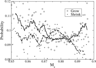
Figure 1: Growing and shrinking probabilities versus the magnetization along the $z$-axis for a 6$\times$6$\times$90 pillar. Grow/shrink data were collected into 6000 bins, which span the entire magnetization axis, [-1,1]. The simulation was run at 20 K, 1125 Oe, and the applied field was directed along the long axis of the pillar, antiparallel to the initial magnetization. The continuous curves represent nine-point running averages

Projective dynamics involves analyzing the probability of growing toward the stable equilibrium or shrinking away from it, as a function of a single variable that measures the progress of the reversal process. To collect growing and shrinking statistics here, the $z$-component of the total magnetization of the pillar, $M_{z}$, was recorded at each integration step. In addition, the change in this value from the previous integration step, $\Delta M_{z}$, was also recorded. The magnetization axis was discretized into bins into which the collected data were sorted. The bin size was determined such that the discretized $\Delta M_{z}$ would only involve changes between adjacent bins. The growing and shrinking probabilities were calculated by counting the number of times that $\Delta M_{z}$ would cause the magnetization to change bins. Define $G$ as the number of times the magnetization hopped to the next bin in the direction toward equilibrium, and $S$ as the number of hops in the direction back toward the metastable state. If $N$ is the total number of visits to the starting bin, then the growing and shrinking probabilities for each bin, $P_{G}$ and $P_{S}$, can be written respectively as

$$P_{G}=\frac{G}{N},\qquad P_{S}=\frac{S}{N}.$$ (2)

The crossings of the growing and shrinking probabilities give information about the locations of the metastable free-energy minimum and the saddle point. Where the two probabilities are equal, the system has no preferred direction of magnetization evolution, indicating that the free-energy landscape is flat in this region. This is the location of an extremum. The right-hand intersection in Fig. 1 corresponds to the metastable free-energy minimum, where the system spends most of its time. At the saddle point, the growing and shrinking probabilities are also equal, as indicated by the left-hand crossing. The region between these two crossings shows a higher probability for shrinkage than growth, corresponding a preference for moving toward the metastable minimum.

Previous simulations performed on a one-dimensional chain of seventeen spins exhibited Stoner-Wohlfarth behavior for the angular dependence of the switching field 5 . This is not representative of experimental data 4 ; 8 ; 9 . However, a full three-dimensional model qualitatively produced the proper angular dependence 5 . This is not surprising, given that the full three-dimensional model allows for magnetization curling modes which are simply not allowed in the one-dimensional model. PD has previously been applied to the one-dimensional spin chain 2 , but several thousand switches had to be performed in order to accumulate sufficient statistics to reveal the free-energy extrema 2 . With typical switches taking around 1500 CPU-hours for the full three-dimensional model, it was not clear that sufficient statistics could be generated.

Figure 1 shows the results collected from only 20 switches for the full model. The estimated $P_{G}$ is shown as circles, and $P_{S}$ as crosses. Scatter in these data is primarily due to the counting statistics and the small number of samples in each bin. Nine-point running averages are used to reduce the scatter and improve estimates of the crossings of $P_{G}$ and $P_{S}$. The running averages are represented by curves and are sufficient to determine the locations of the extrema with an uncertainty of about $1\times 10^{-3}$ in the magnetization. For the one-dimensional model the estimated curves representing $P_{G}$ and $P_{S}$ are almost parallel near the saddle point, making it difficult to locate crossings of the growing and shrinking probabilities (see Fig. 1 of Ref. 2 ). Since they cross at a significant angle for the model studied here (see Fig. 1), it is possible to find an estimate for the magnetization of the free-energy saddle point from far fewer switches than were needed for the one-dimensional model.

III Summary and Conclusions

The projective dynamics method was used to produce growing and shrinking probabilities during the magnetization reversal of a realistic model nanopillar. These probabilities can be used to locate the magnetization of the free-energy extrema. In particular, the magnetization of the saddle point is revealed. Compared to the one-dimensional model, far fewer switches are needed to find the location of the extrema in the three-dimensional model. In the future, a study of the dependence of the saddle point on temperature and misalignment between the pillar and the applied field are planned.

References

- (1) M.A. McCord, D.D. Awschalom: Appl. Phys. Lett. 57, 2153 (1990)
- (2) M. Kolesik, M.A. Novotny, P.A. Rikvold, D.M. Townsley, in: Computer Simulation Studies in Condensed Matter Physics X., Ed. by D.P. Landau, K.K. Mon, and H.-B. Schüttler (Springer-Verlag, Berlin 1998) p. 246
- (3) G. Brown, M.A. Novotny, P.A. Rikvold: Physica B 343, 195 (2003)
- (4) G. Brown, S.M. Stinnett, M.A. Novotny, P.A. Rikvold: J. Appl. Phys. (in press). E-print arXiv: cond-mat/0310497
- (5) S. Wirth, S. von Molnár: Appl. Phys. Lett. 76, 3283 (2000); 77, 762 (2000)
- (6) S. Wirth, M. Field, D.D. Awschalom, S. von Molnár: Phys. Rev B 57, R14028 (1998)
- (7) Y. Li, P. Xiong, S. von Molnár, Y. Ohno, H. Ohno: Appl. Phys. Lett. 80, 4644 (2002)
- (8) W.F. Brown: IEEE Trans. Magn. 15, 1196 (1979)