Singular dynamics and pseudogap formation in the underscreened Kondo impurity and Kondo lattice models
Abstract
We study a generalization of the Kondo model in which the impurity spin is represented by Abrikosov fermions in a rotation group SU() larger than the SU() group associated to the spin of the conduction electrons, thereby forcing the single electronic bath to underscreen the localized moment. We demonstrate how to formulate a controlled large limit preserving the property of underscreening, and which can be seen as a “dual” theory of the multichannel large equations usually associated to overscreening. Due to the anomalous scattering on the uncompensated degrees of freedom, the Fermi liquid description of the electronic fluid is invalidated, with the logarithmic singularities known to occur in the SU(2) Kondo impurity model being replaced by continuous power laws at . The present technique can be extended to tackle the related underscreened Kondo lattice model in the large limit. We discover the occurence of an insulating pseudogap regime in place of the expected renormalized metallic phase of the fully screened case, preventing the establishement of coherence over the lattice. This work and the recent observation of a similar weakly insulating behavior on transport in CeCuAs2 should give momentum for further studies of underscreened impurity models on the lattice.
I Introduction
The Kondo model, initially introduced to describe with great success the behavior of diluted magnetic impurities in metals Hewson (1996), has been an exciting playground for condensed matter physicists in the last two decades. Indeed, the extreme simplicity of this many-body Hamiltonian was key to some unexpected progresses in the field, such as the discovery of the effective theory describing the Mott transition Georges et al. (1996), and as a prototypal description of Non Fermi liquid behavior in multi-channel Nozières and Blandin (1980) and pseudogap extensions Bulla and Vojta (2003). Localized quantum impurities also provide the building entity to describe heavy fermion materials Lee et al. (1986), and this is still a strong motivation for studying Kondo models on the lattice, most interestingly in relation to the violation of Fermi liquid behavior associated to the breakdown of Kondo screening close to a quantum critical point Stewart (2001), as discovered in a wide class of -electron metals such as CeCu6-xAux Schröder et al. (2000). Interest in the Kondo model was also revived by the possibility of building and controlling precisely quantum impurity states in semiconducting devices, leading to the realization of the Kondo effect in quantum dots Kouwenhoven and Glazman (2001). The possibility of observing Non Fermi liquid behavior in a multi-channel setup was recently advocated Oreg and Goldhaber-Gordon (2003); Florens and Rosch (2004); Anders et al. (2003), and provides further incentive for a complete understanding of quantum impurity problems.
Quite recently, peculiar attention was given to the Kondo problem by Coleman and Pepin Coleman and Pépin (2003), in the study of an underscreened model which showed relatively strong deviations from Fermi liquid behavior in the specific heat (we point out however that related effects can be traced back to the physics of the ferromagnetic Kondo model Giamarchi et al. (1993), see also Schlottmann (2000)). This surprising result was interpreted as due to anomalous scattering of conduction electrons onto the remaining unscreened spin degrees of freedom, giving rise to a “singular” Fermi liquid fixed point, which differs from the intermediate fixed point Nozières and Blandin (1980); Florens (2004) associated to usual Non Fermi liquid by the fact that the effective ferromagnetic Kondo coupling renormalizes to zero at low energy Nozières and Blandin (1980). This insightful work was however limited to a range of frequencies higher than the Zeeman energy, and concentrated mainly on thermodynamic quantities. In order to study in more detail the dynamics due to these anomalous excitations in the underscreened Kondo model, we would like to find a simple approach that would be able to grasp the full crossover from the local moment regime at high temperature down to the underscreened state in which nearby conduction electrons are tightly bound to the impurity. In the realistic case of SU(2) spins, we note that the deviation from exact screening can be in principle tuned Nozières and Blandin (1980) by changing the size of the impurity spin and/or the number of screening channels , obtaining a transition from underscreening at to overscreening at (with perfect screening at ).
A simple route to capture this physics consists in establishing a large limit of the problem, generalizing the quantum spin to the SU() group. A crucial step lies however in the choice of the SU() representation in which the spin is considered. It is known that fermionic representations at large only allow perfect screening when Coleman (1987) and overscreening otherwise Cox and Ruckenstein (1993); Parcollet et al. (1998). Interestingly, bosonic representations of SU() preserve the distinction between “small” and “large” spin as found by Parcollet and Georges Parcollet and Georges (1997), and allow to study the underscreened situation. However, this case presents some pathologies: the T-matrix scales as , and the singular behavior as found in Coleman and Pépin (2003) seems to be absent of the solution Georges .
The previous discussion illustrates the need for an alternative large limit to describe the underscreened Kondo effect, but also gives momentum to the idea we will pursue in the following. Indeed, we can understand that overscreening and underscreening are somewhat “dual” in the sense that, while the former situation is reached in the presence of many screening channels, the latter case should be obtained by considering many “spin channels”. A simple way to formalize this is to strongly enlarge the symmetry group of the impurity spin, thus forcing underscreening by the bath of conduction electrons. In fact, if one considers a generalized Kondo model involving a single bath of SU() electrons interacting with a localized SU() spin, where is larger than , one expects underscreening, independently of the representation chosen for the impurity. Because the -channel large limit which describes overscreening is obtained for Cox and Ruckenstein (1993); Parcollet et al. (1998), we can guess that a reasonable large limit of underscreening can be found when ( being the number of “spin channels”). We will show that the saddle-point equations derived in this way at present a “dual” structure to the Non Crossing Approximation associated to the overscreened case Bickers (1987); Cox and Ruckenstein (1993); Parcollet et al. (1998), and reveal non Fermi liquid behavior with a continuously varying exponent parametrized by the ratio . The lattice version of this generalized underscreened Kondo model is also straightforwardly solvable, due to the absence of generated RKKY interactions. Because singular scattering of delocalized electrons on the degenerate manifold of unscreened spin occurs, coherence cannot establish over the lattice, in contrast to the exactly screened Kondo lattice Auerbach and Levin (1986). This proves the existence of a generic insulating-like state with a pseudogap density of states, parametrized by the same anomalous exponent unveiled in the single impurity underscreened Kondo model. We conclude the paper by future prospects regarding the theory of underscreened Kondo models, and by the possible observation of their physical consequences in strongly correlated materials, pointing out some similarities with the cerium based compound CeCuAs2, on which transport measurements were recently reported.
II Novel large limit of the underscreened Kondo model
II.1 Model
Our aim in this section is to introduce a Kondo model in which the underscreened aspect is built in from the beginning, while a simple large limit of the problem can be found by proper rescaling of the parameters.
II.1.1 Heuristic derivation
The basic idea, which was presented in the introduction, is to consider a single-channel Kondo Hamiltonian involving conduction electrons with spin flavors and interacting with a SU() spin localized at the origin:
| (1) |
where , . The matrix of coupling constants will be specified in the following. We choose a completely antisymmetric representation of the spin using Abrikosov fermions:
| (2) | |||||
| (3) |
where the second equation is the necessary constraint to enforce the spin size (this scaling, where is of order 1, is necessary to get a large limit, see below). As emphasized previously, leads to underscreening, and a likely scaling to obtain a solvable limit is . Let us therefore set , with , expressing fermions in a double index notation:
| (4) |
where represents the doublet of indices , with . Neglecting potential scattering terms, which only contribute to next order in , the Hamiltonian now reads:
| (5) |
This is now completely general, and we would like to chose the simplest coupling between the itinerant SU() fermions and the localized SU() spin. In the spirit of having “spin channels”, we set:
| (6) |
and obtain the Hamiltonian
| (7) | |||||
| (8) |
associated with the single constraint eq. (8). This will be our starting point for the large solution.
II.1.2 Alternative interpretation
One might argue that coupling a band of fermions to a spin with a different symmetry group is not a very transparent concept on a physical point of view. Indeed, one can try to view alternatively the Hamiltonian (7) as the standard SU() Kondo model with a localized SU() spin taken in a rectangular representation Kiselev et al. (2001) of size :
| (9) |
Usual Kondo coupling to the SU() electronic bath leads indeed to the Hamiltonian (7). We will however not pursue this route in the present work, as this type of representation asks to consider a set of constraints:
| (10) |
which makes the large limit impracticable. We will come back to the differences between the large group technique (developed in this work) and the rectangular representation approach in section III.3.2, while discussing the physical results.
II.2 Derivation of the saddle-point equations
In order to solve the model (7-8), we first write the imaginary time action of the problem with inverse temperature :
| (11) | |||||
introducing a Lagrange multiplier to enforce the constraint (8). The precise form of the action (11) is hinting that a large solution is possible, which we perform now.
The following step is to decouple the interaction with a bosonic field :
and integrate out the fermions :
where , with . We finally introduce the electron sitting at the impurity center, , so that:
where . Because scales as , the existence of a saddle-point is manifest in the previous expression. Following Parcollet et al. (1998), we find the integral equations:
| (16) | |||||
| (17) | |||||
| (18) | |||||
| (19) |
where is a bosonic Matsubara frequency.
II.3 Interpretation of the formalism
Let us first comment on the formal analogy that the system of equations (LABEL:Gc-18) shares with the usual Non Crossing Approximation (NCA) Bickers (1987); Cox and Ruckenstein (1993); Parcollet et al. (1998). We notice indeed that the roles of the local bath electron and of the Abrikosov fermion are simply exchanged with respect to the usual NCA structure, which, we recall, is associated to overscreening Parcollet et al. (1998). In particular, the self-energy now involves the propagator instead of in the NCA, and this difference will be shown below to radically affect the physics, with the occurence of underscreening instead of overscreening. This interesting “duality” is one of the main results of the present work.
It is also very appealing to remark that the computation of physical observables related to the itinerant band does not involve directly pseudo-fermion degrees of freedom, contrarily to the multichannel case. Indeed, the present theory is formulated directly in terms of the bath propagator, to which the T-matrix is simply related by the relation:
If we sum the previous expression over all momenta, we find:
| (22) | |||||
| (23) |
where (LABEL:Gc) was used to obtain the second expression. Interestingly, we note that the T-matrix (23) is of order in the present scheme, whereas it happens to scale as in the multi-channel large limit Parcollet et al. (1998), a certain drawback for the theory of overscreening. However, by the “duality” argument, we expect to find that the spinon propagator only shows corrections to the free impurity limit (), which can indeed be easily checked by a direct computation:
| (24) | |||||
| (25) |
This means that, although the T-matrix is conveniently captured by the present scheme, computation of e.g. the spin susceptibility involves necessarily corrections. This remark allows however to solve explicitely the constraint equation (19) at the leading order:
| (26) | |||||
| (27) |
III Physical study of the non Fermi liquid regime
III.1 At particle-hole symmetry
For simplicity, we start with the assumption of particle-hole symmetry, (the free bath will always be assumed symmetric in the following). This implies that the constraint (19) is fulfilled provided , and we have:
| (28) |
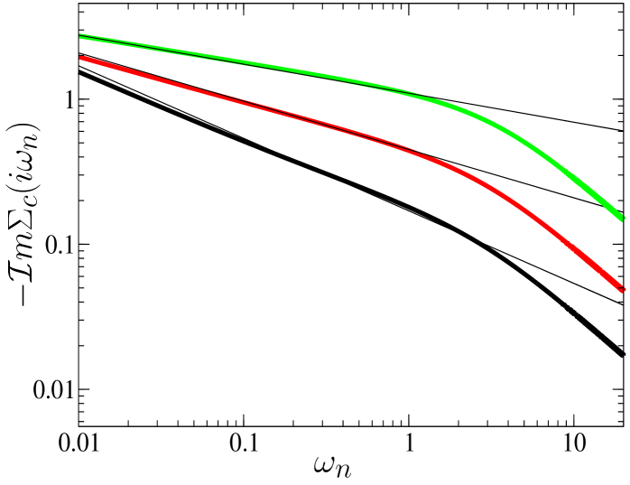
i.e. long range correlations in the self-energies (17-18). By analogy with the low-frequency analysis usually performed in studying the NCA equations Mueller-Hartmann (1984); Parcollet et al. (1998), we assume power law behavior of the self-energies and plug into the saddle-point equations. Self-consistency can be achieved at zero temperature (see Appendix A) and we obtain for real frequency quantities:
| (29) | |||||
| (30) | |||||
| (31) |
where and are undetermined constants. This analytical result is well borne out by the numerical solution of the saddle point equations as shown by figure 1 (in the following computations, a semi-circular density of states with half-width was chosen to model the bath of conduction electrons).
We would like to contrast this peculiar low energy behavior with the one observed in a standard Fermi liquid (as in the fully screened Kondo model). The interpretation of these results can be made clearer by considering the T-matrix of a related Anderson model:
| (32) |
where the local fermion has an hybridization to the -electrons and is subject to a local Coulomb repulsion term (and possibly to a strong Hund’s rule if one wants to stabilize a spin in order to make the connection to the underscreened case), giving rise to the term in the previous equation. Comparing (23) and (32), we see that the inverse self-energy of the bath electrons is simply related to the impurity self-energy by . In a Fermi liquid, we know Hewson (1996) that the impurity self-energy obeys at low frequency:
| (33) |
where is the quasiparticle residue and the inelastic scattering rate. The previous general identification between and provides the self-energy of the local electron in the bath for a Fermi liquid:
| (34) |
the first term corresponding to regular elastic scattering from the impurity. The fact that this self-energy diverges as a power law at low frequency in the underscreened case (29) signals anomalous scattering on the remaining unscreened degrees of freedom, which ultimately violates the Fermi liquid description of the problem. This result can be more clearly witnessed from the impurity self-energy itself
| (35) |
showing a power law scattering rate for the localized state which even dominates the linear part found in the self-energy of a Fermi liquid, equation (33). Indeed, we deduce from this behavior a frequency dependent quasiparticle residue which vanishes at low energy, demonstrating a clear breakdown of Fermi liquid theory.
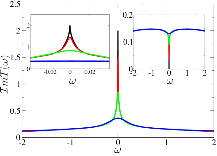
A final way to put into evidence the singular energy dependence of this underscreened impurity is to compute the T-matrix. We find indeed that the Kondo resonance, whose development is illustrated on figure 2, displays a cusp at low frequency:
| (36) |
using in equation (23) the low frequency behavior of the free Green’s function, . This expression shows that, although the unitary limit is recovered in the T-matrix at , Fermi liquid behavior is nevertheless violated by the non-analytic expansion a low frequency.
III.2 Away from particle-hole symmetry
Here we discuss briefly the case , and investigate whether the previous results remain valid when particle-hole symmetry is broken. The propagator appearing in the bubble giving the self-energies, equations (17-18), is given by:
| (37) |
and decays exponentially. We argue that the long range correlations which are crucial to maintain the non-trivial power laws are still present, because saturates at low temperature, from (27). This would imply that the non Fermi liquid state survives the introduction of the asymmetry parameter , as can also be verified from the numerics.
However, the structure of the saddle point is such that the constraint (8) scales as instead of , and hints that it might be necessary to account for corrections to the result (27). We do not find that this possibility really modifies the previous result, , although we think this question deserves further clarification.
III.3 Discussion: theoretical aspects
III.3.1 Possible extensions of the formalism
The present approach seems well suited to describe the underscreened situation of quantum impurity models. We can however point out two kinds of limitations, which are in fact also inherent to the Non Crossing Approximation of multichannel models as well Parcollet et al. (1998). First, although the T-matrix can now be naturally extracted at the saddle-point level, some physical quantities such as the spin susceptibility appear only at next to leading order in 1/. Second, motivated by some puzzles raised in heavy fermion compounds, it remains of great interest to develop faithfull large expansion methods that can work in the exactly screened case too (an interesting step in this direction was however taken in Parcollet and Georges (1997)). It was in fact already acknowledged Parcollet that a simple generalization of the Kondo model is quite suitable for overcoming both of these difficulties: it consists in taking the localized spin in a rectangular representation of SU(), as indeed done in the present work (if one were able to take good care of the necessary constraints, see discussion in section II.1.2), while assuming also a large number (of order ) of screening channels (in this paper we only considered the single channel case). This extension of the formalism, also known as “matrix Kondo model”, leads however to technical difficulties due to proliferation of Feynman graphs at large . It is actually possible to resum this complicated diagrammatics using a soft constraint approach inspired by a recent study Florens and Rosch (2004) of the interplay of Kondo effect and Coulomb blockade (viewed now as a purely mathematical trick). Such a theory would be a bridge between the usual large approach of overscreening and the present work, both appearing as simple limitating cases of it, thus finding an unity behind our “duality” picture. Such a theory will be considered in a forthcoming publication Florens
III.3.2 On the nature of the low energy singularities
As we have demonstrated from the analytical and numerical solution of the new large-N equations, the underscreened Kondo impurity model displays violations of low energy Fermi liquid behavior, although those are less severe as the one observed in the overscreened case (where the deviation from the unitary limit associated to finite lifetime of the electrons at zero temperature even dominates the anomalous frequency dependence of the scattering rate). The underscreened impurity is nevertheless associated to Non Fermi liquid behavior: the local quasiparticle weight vanishes at low energy and the system presents additional degeneracy due to the non fully screened spin. It is interesting to compare this result to previous exact knowledge from the Bethe ansatz solution of underscreened Kondo models. Although the general features we have sketched so far are indeed obtained from the Bethe ansatz analysis, one crucial difference concerns the precise nature of the singular frequency dependence of the physical quantities: while we observe universal non-trivial exponents in the large N solution, the SU(2) Kondo model rather displays logarithmic behavior Coleman and Pépin (2003) (although power laws are actually found in the anisotropic case Schlottmann (2000)). We think this difference is a minor point, that we would naively like to attribute to special features associated to the large N generalization of the model. This point is actually more subtle. Indeed , the hamiltonian (7) we have solved can be argued (see section II.1.2) to be equivalent to a SU() Kondo model with spin in a rectangular representation, which is actually diagonalized by Bethe ansatz Zinn-Justin and Andrei (1998), and found to display also logarithmic singularities! As stressed previously, we have however enforced a different type of constraint in the present approach, and we would ultimately pin point this difference to be the origin of the discrepancy in the low energy behavior as compared to the exact solution. This discussion would tend to illustrate in any case the fact that the physics can be sensitive in how the constraint is implemented, but we will reinforce our judgment that the present method captures the essential features of underscreening. As we will now demonstrate, the main interest of our approach is that it can apply to problems where no exact solution is available, in particular in the many impurities extension of the underscreened Kondo model.
IV Pseudogap formation in the underscreened Kondo lattice
IV.1 Model and large solution
We introduce here the lattice extension of the previous single impurity model, which consists of a dense network of impurities carrying a SU() spin on which a band of SU() itinerant electrons scatter:
| (38) |
Here labels sites, with , is the chemical potential in the -band and other conventions are similar to previously. This model is not very realistic in many respects, and to date lacks a physical realization in condensed matter systems (see however the ending discussion in section IV.4). On a purely theoretical point of view, we can raise however two interesting questions. First, what is the behavior of the electronic band below the Kondo temperature associated to underscreening? For this to make sense, we need to argue that the magnetic processes involving the remanent spin degrees can be ignored, for example due to frustration (maybe by analogy to the compound LiV2O4). Second, when the partially-screened local moments start to order, and quench their macroscopic entropy, how does the system behaves? In the following large analysis of this problem, we will see that intersite magnetic correlations are absent, and that the first of these questions can be answered.
The large limit is derived following the same steps performed in section II, introducing local bosons to decouple the Kondo term on each site, and integrating the Abrikosov fermions:
We can simply read off this expression the final saddle point equations, which are completely identical to (16-18), except that the local bath propagator now reads:
| (40) | |||||
| (41) |
IV.2 Interpretation
The new system of integral equations (16-18),(41) is remarkably simple in its structure, a fact due to the absence of intersite correlations at this level of approximation. Indeed, as the action (IV.1) shows, no magnetic RKKY interaction is generated at the saddle-point level, which is expected since the additional quantum number carried by the localized spins cannot be transported from site to site by the itinerant fermions. We point out however that this is not a general feature of underscreened models, and one can easily check that the RKKY interaction is indeed mediated by the electronic bath in the finite SU(2) case.
Besides, expression (41) is reminiscent of a self-consistent T-matrix approximation and signals that electrons in the bath are still anomalously scattered by the localized spins, acting independently of each other. Indeed, if we assume that is divergent as in the single impurity case, equation (29), we see that this singular self-energy dominates the -summation in (41) at low energy, so that:
| (42) |
with the same exponent (31) as found previously. This means that in the underscreened Kondo lattice, there is no important distinction between the cases of dense and diluted impurities (on the point of view of the bath electrons that feel the Kondo interaction), and that the itinerant electron density of states always shows a pseudogap at low energy. This is quite different from the situation of exactly screened models, where a hard hybridization gap would open at half-filling. In the perfectly screened case, coherence can always be re-established upon doping, despite the fact that each individual impurity scatters strongly the electrons. The result (42) would however let us think that electronic degrees of freedom always remain confined in the underscreened Kondo lattice, as we now check on the numerical solution of the saddle-point equations.
IV.3 Results
We will be again interested in the T-matrix, which is related to the (translation invariant) -electron Green’s function by:
| (43) |
This relation can be best understood from an equivalent periodic Anderson model, where is proportional to the momentum- and frequency-dependent Green’s function of the localized electrons. From the effective action (IV.1) we have:
| (44) |
so that the T-matrix can be expressed as:
| (45) |
Again, we identify as the impurity self-energy (up to a factor ). The local T-matrix, is easily calculated from (45) after the numerical solution of the saddle-point equations, and is shown in Figure 3 (here also a semi-circular density of states for the -electron was taken).
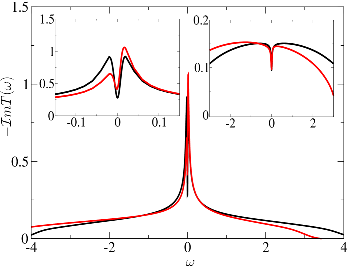
From the numerical solution, and in agreement with the previous analytical analysis, we see that an hybridization pseudogap opens in the spectrum, irrespective of the filling of the -band. This prevents coherence to be reached over the lattice at zero temperature (note that Figure 3 is performed at finite temperature, so that the pseudogap in the density of states is filled by thermal excitations). Therefore, the strongly underscreened Kondo lattice is strictly speaking an insulator, with a resistivity likely showing a power law increase as temperature is lowered, instead of the activated or metallic behavior expected respectively in usual Kondo insulators or in heavy fermion metals. In order to shed some light onto this remarkable result, we put it into the perspective of previous theoretical work and experimental measurements on a newly discovered -electron material.
IV.4 Physical discussion
IV.4.1 Underscreened Kondo lattice: status of theory
The main physical result of the paper is that the underscreened Kondo lattice is an insulator with a pseudogap density of states above the ordering temperature of the partially screened moments, for all filling of the electronic band. Theoretically, we can ask whether this behavior is peculiar to the large solution performed here or can be expected to be generic. To answer this question, it is interesting to notice two facts. First, previous work by K. Le Hur in a one dimensional model of underscreened Kondo ladder LeHur (1999) demonstrated infact similar insulating behavior (this quite peculiar model was chosen in order to prevent the Haldane spin gap associated to the 1D chain, which would pollute the interesting physics). Second, our large solution displays actually some high dimensional features Georges et al. (1996), such as a local self-energy, as seen in equation (44). Because this insulating behavior is found in two such extreme cases, we could expect for a continuity of this non-metallic behavior of underscreened lattice in intermediate dimension also.
We now turn to the nature of this insulating state. As discussed in the single impurity case, section III.3.2, the large solution predicts that the dynamics is governed by universal power law behavior rather than the logarithmic singularities found in the SU(2) case and extensions, although the physics of these anomalies can be expected to be similar. This discussion extends naturally to the underscreened lattice, and deserves clearly further theoretical studies. We think that a next step could be taken by solving the Kondo lattice model in a combination of DMFT Georges et al. (1996) and NRG techniques, and would help both to confirm the generic insulating behavior found here, and investigate in more detail the physical properties that are associated to it.
IV.4.2 Physical observation of the underscreened Kondo effect
We finally discuss the possible experimental realization of underscreened Kondo physics. Concerning the single impurity case, the stability of for quantum dots in even valleys of Coulomb blockade was discussed both theoretically and experimentally (for a review, see Pustilnik and Glazman (2004)), although no emphasis was put onto the singular behavior that we have discussed previously. Another way to observe Kondo underscreening would be to study large atoms deposited on a metallic surface and scanned by an STM tip.
Finding an -electron material related to the underscreened Kondo lattice seems to be a more daunting task. Indeed, not only the intersite magnetic correlations would need to be small in such a system, but a mechanism to form large spin (or spin-orbital degeneracy) of the -level should be invoked. Typically, crystal fields leave unfortunately an effective Kramers doublet below temperature of several dozens of Kelvins. However, we think that the present work is interesting since it highlights the peculiar physical properties of underscreened lattices, and may be useful in strengthening an eventual experimental observation. In fact, very recent transport measurements of a new cerium based compound, CeCuAs2, revealed weakly insulating behavior of the resistivity, with a power law divergence at low temperature Sengupta et al. (2004). While we are careful in connecting hastily this observation to our theoretical findinds, we hope that these remarks would stimulate further studies of underscreening effects in Kondo systems.
V Conclusion
The underscreened Kondo model was investigated in this paper by means of a specially developed large technique. Although the strong coupling fixed point in which itinerant electrons are tightly bound to the uncompensated spin is stable in the renormalization group sense, we have shown that non Fermi liquid behavior appears in the form of anomalous power laws in the physical observables. The universal exponent was computed analytically and checked over the numerical solution of integral equations, which show an interesting duality with respect to the previous theory of overscreening in multichannel models. The extension to a finite dimensional lattice of underscreened magnetic moments was also considered, and a pseudogap (weakly insulating) regime was discovered, with similar power laws governing the dynamics of the electrons. We have also tried to point out several directions for future research, both concerning the theoretical aspects of underscreened models and their experimental realization, for which CeCuAs2 might be a candidate.
Acknowledgements.
I wish to thank Matthias Vojta for some useful suggestions at the early stages of this work, and for comments on the manuscript. I am also grateful to E. V. Sampathkumaran for communicating his experimental results before publication Sengupta et al. (2004). Financial support by the Center for Functional Nanostrutures is also acknowledged. During the completion of the present paper, a similar large limit of the underscreened Kondo model was proposed by P. Coleman and I. Paul Coleman and Paul (2004), with results complementary to ours in the single impurity case. A very detailed investigation of the singularities occuring in the SU(2) Kondo model was also carried out simultanenously by P. Mehta et al. Mehta et al. (2004) using a combination of Bethe ansatz and Numerical Renormalization Group techniques.Appendix A
We present here the derivation of the non-trivial exponent governing the low frequency behavior of the physical quantities, following Parcollet et al. (1998); Mueller-Hartmann (1984). Let us assume the ansatz:
| (46) | |||||
| (47) |
at zero temperature. Using the spectral decomposition:
| (48) |
and the expression for the self-energies (17-18) with , we find:
| (49) | |||||
| (50) |
Going back to frequency, we have simply:
| (51) | |||||
| (52) |
To determine the real part in the previous self-energies, we use an analyticity argument, which gives for complex frequency :
| (53) | |||||
| (54) |
and similarly for and . Finally, from Dyson’s equation (LABEL:Gc)-(16), we have and , providing relations between amplitudes , and exponents , . After some manipulations, we find:
| (55) |
References
- Hewson (1996) A. Hewson, The Kondo problem to heavy fermions (Cambridge, 1996).
- Georges et al. (1996) A. Georges, G. Kotliar, W. Krauth, and M. Rozenberg, Rev. Mod. Phys. 68, 13 (1996).
- Nozières and Blandin (1980) P. Nozières and A. Blandin, J. Physique 41, 193 (1980).
- Bulla and Vojta (2003) R. Bulla and M. Vojta, in Concepts in Electron Correlations, A.C. Hewson and V. Zlatic (eds.), Kluwer Academic Publishers, Dordrecht (2003), eprint cond-mat/0210015.
- Lee et al. (1986) P. A. Lee, T. M. Rice, J. W. Serene, L. J. Sham, and J. W. Wilkins, Comment. Cond. Mat. Phys. 12, 99 (1986).
- Stewart (2001) G. R. Stewart, Rev. Mod. Phys. 73, 797 (2001).
- Schröder et al. (2000) A. Schröder, G. Aeppli, R. Coldea, M. Adams, O. Stockert, H. von Löhneysen, E. Bucher, R. Ramazashvili, and P. Coleman, Nature 407, 351 (2000).
- Kouwenhoven and Glazman (2001) L. Kouwenhoven and L. Glazman, Physics World 14, 33 (2001).
- Oreg and Goldhaber-Gordon (2003) Y. Oreg and D. Goldhaber-Gordon, Phys. Rev. Lett. 90, 136602 (2003).
- Florens and Rosch (2004) S. Florens and A. Rosch, Phys. Rev. Lett. 92, 216601 (2004).
- Anders et al. (2003) F. B. Anders, E. Lebanon, and A. Schiller (2003), eprint cond-mat/0311502.
- Coleman and Pépin (2003) P. Coleman and C. Pépin, Phys. Rev. B 68, 220405 (2003).
- Giamarchi et al. (1993) T. Giamarchi, C. M. Varma, A. E. Ruckenstein, and P. Nozières, Phys. Rev. Lett. 70, 3967 (1993).
- Schlottmann (2000) P. Schlottmann, Phys. Rev. Lett. 84, 1559 (2000).
- Florens (2004) S. Florens, Phys. Rev. B 69, 113103 (2004).
- Coleman (1987) P. Coleman, Phys. Rev. B 35, 5072 (1987).
- Cox and Ruckenstein (1993) D. L. Cox and A. E. Ruckenstein, Phys. Rev. Lett. 71, 1613 (1993).
- Parcollet et al. (1998) O. Parcollet, A. Georges, G. Kotliar, and A. Sengupta, Phys. Rev. B 58, 3794 (1998).
- Parcollet and Georges (1997) O. Parcollet and A. Georges, Phys. Rev. Lett. 79, 4665 (1997).
- (20) A. Georges, private communication.
- Bickers (1987) N. E. Bickers, Rev. Mod. Phys. 59, 845 (1987).
- Auerbach and Levin (1986) A. Auerbach and K. Levin, Phys. Rev. Lett. 57, 877 (1986).
- Kiselev et al. (2001) M. N. Kiselev, H. Feldmann, and R. Oppermann, Eur. Phys. J B 22, 53 (2001).
- Mueller-Hartmann (1984) E. Mueller-Hartmann, Z. Phys. B 57, 281 (1984).
- (25) O. Parcollet, ph. D Thesis, Paris VI University.
- (26) S. Florens, in preparation.
- Zinn-Justin and Andrei (1998) P. Zinn-Justin and N. Andrei, Nucl. Phys. B B528, 648 (1998).
- LeHur (1999) K. LeHur, Phys. Rev. Lett. 83, 848 (1999).
- Pustilnik and Glazman (2004) M. Pustilnik and L. Glazman, J. Phys: Condens. Matter 16, R513 (2004).
- Sengupta et al. (2004) K. Sengupta, E. V. Sampathkumaran, S. Rayaprol, T. Nakano, M. Hedo, M. Abliz, N. Fujiwara, Y. Uwatoko, K. Shigetoh, T. Takabatake, et al., Phys. Rev. B 70, 064406 (2004).
- Coleman and Paul (2004) P. Coleman and I. Paul (2004), eprint cond-mat/0404001.
- Mehta et al. (2004) P. Mehta, L. Borda, G. Zarand, N. Andrei, and P. Coleman (2004), eprint cond-mat/0404122.