Stoner-Wohlfart model applied to bicrystal magnetoresistance hysteresis

Abstract

We calculate numerically the magnetization direction as function of magnetic field in the Stoner-Wohlfart theory and are able to reproduce the shape of the low-field magnetoresistance hysteresis observed in manganite grain boundary junctions. Moreover, we show that it is necessary to include biaxial magnetocrystalline anisotropy to fully describe the grain boundary magnetoresistance in La_0.7Sr_0.3MnO₃/SrTiO₃ bicrystal tunnel junctions.

Can the fairly simple model presented by Stoner and Wohlfart in 1948 Stoner and Wohlfarth (1948) provide insights in the processes that occur in manganite bicrystal grain boundary junctions? In the following we show how the coherent rotation of the magnetization vector can explain the characteristic features in the field dependence of the magnetoresistance.

Recently, a substantial low-field magnetoresistance was observed in grain boundaries of perovskite manganites Hwang et al. (1996); Gupta et al. (1996) and other half-metallic ferromagnets Hwang and Cheong (1997); Yin et al. (2000). In order to understand and exploit this effect several studies have used bicrystal grain boundary junctions Mathur et al. (1997); Steenbeck et al. (1997); Gross et al. (2000). Since bicrystals are samples with well defined crystal orientations with respect to an interface, they are in a way ideal systems for studies of the behaviour of magnetic tunnel junctions. Traditionally, the conductivity of magnetic tunnel junctions is compared with Julliere’s model Julliere (1975), in which the tunneling magnetoresistance is determined by the spin polarization of the electrodes. A more realistic scenario was considered by Slonczewski Slonczewski (1989), who used a method to match the wave functions across the tunneling barrier. He derived an expression for direct tunneling through the interface which includes the angle between the directions of the magnetization of the electrodes.

However, direct tunneling is not sufficient to explain the measured transport data in manganite grain boundary junctions. In fact, even though several scenarios have been suggested to explain measured data, the transport mechanism in bicrystal grain boundaries of manganites is still not fully understood. Klein, Höfener and coworkers Klein et al. (1999); Höfener et al. (2000) pointed out the strong impact of inelastic processes in the barrier region. They concluded that multi-step tunneling via a number of localized states within the barrier had to be added to the elastic tunneling conductivity contribution. Several different inelastic processes have been suggested in order to explain experimental data, most of them emphasizing scattering at magnetic intra-barrier states Guinea (1998); Lee et al. (1999); Ziese (1999).

So far, most studies of the transport mechanism in manganite grain boundaries have focused on the non-linearity of the $I-V$-curves, the magnitude of the low-field magnetoresistance or the shape of the magnetoresistance at high fields. The shape of the low-field hysteresis, directly related to the magnetization reversal process at the grain boundary, has long been neglected. Recently however, one attempt to reproduce the hysteresis was presented: García and Alascio García and Alascio (2002) minimized the total magnetic energy and obtained the magnetoresistance from the magnetization directions. They considered the energy within the grain boundary region, and assumed uniaxial anisotropy in order to reproduce the experimental data.

In this paper we explore the possibility to describe the low-field magnetoresistance in a bicrystal junction in terms of coherent rotation of the magnetization directions, similar to what was presented more than half a century ago by Stoner and Wohlfart Stoner and Wohlfarth (1948). In a numerical calculation we demonstrate that the shape of the hysteresis in the magnetoresistance can be obtained by a simple energy-minimization technique, where each grain is treated individually. We show that a biaxial magnetocrystalline anisotropy very well reproduces the measured magnetoresistance curve in a bicrystal grain boundary junction.

In the original paper by Stoner and Wohlfart from 1948 Stoner and Wohlfarth (1948), they described the magnetization reversal of uniformly magnetized ellipsoidal particles. Generally the equilibrium domain structure and magnetization reversal processes are determined by the balance between the exchange, magnetocrystalline, magnetostatic and Zeeman energy contributions (see e.g. Ref. Aharoni (2000)). Let us consider the two-dimensional case of a microbridge crossing a single bicrystal grain boundary, a type of device that has been well studied experimentally. The easy axis of magnetization, the magnetic field $\vec{B}$ and the magnetization $\vec{M}$ are oriented in directions ($\alpha$, $\beta$ and $\gamma$, respectively) defined relative to the grain boundary as depicted in Fig. 1. Furthermore, let us first consider the two single crystal electrode sides (left and right) as being uniformly magnetized and decoupled from each other, i.e. only the variation of the magnetocrystalline and Zeeman energies have to be considered. Hence the field dependent part of the energy density for one of the sides can be written as

$$\omega=\frac{K}{4}\sin^{2}2(\alpha-\gamma)-MB\cos(\beta-\gamma),$$ (1)

where $K$ is the (first order) biaxial anisotropy coefficient. In the case of uniaxial anisotropy the first term should be replaced by Not (a)

$$K_{u}\sin^{2}(\alpha-\gamma).$$

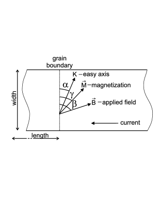
Figure 1: The directions of the easy axis, the applied magnetic field and the magnetization ($\alpha$, $\beta$ and $\gamma$, respectively) are all defined with respect to the grain boundary. The magnetoresistance is measured with the current along the length of the structure.

For fixed values of $K$ and $M$ and the angles $\alpha$ and $\beta$, the magnetization direction $\gamma$ can be obtained from Eq. 1 by tracing a local energy minimum in the $\omega(B,\gamma)$ diagram. The starting point in this numerical method is chosen to be a global minimum at high magnetic field. By stepping the magnetic field we obtain $\gamma(B)$, as shown in Fig. 2. With the assumption that magnetization reversal occurs by coherent rotation and $|\vec{M}|=M_{s}$, where $M_{s}$ is the saturation magnetization, we can trace the rotation of $\vec{M}$ and find $\vec{M}(B)$.

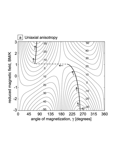
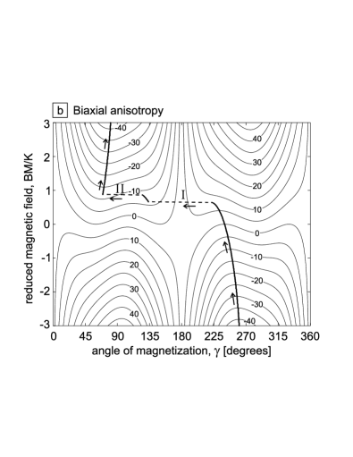
Figure 2: Constant energy contours ($\omega$) calculated from Eq. 1 for constant $K$ and $M$ ($K/M=38$ mT) using a) uniaxial and b) biaxial anisotropy, with $\alpha=60^{\circ}$ and $\beta=90^{\circ}$. The bold line indicates a local minimum traced from $-B_{max}$ to $+B_{max}$, and the direction of rotation is indicated by arrows.

To apply this model to the bicrystal grain boundaries we trace the local minima defined by Eq. 1 for the left and right side independently. Hence we obtain $\gamma_{L}(B)$ and $\gamma_{R}(B)$ for the two sides with easy axis in the direction $\alpha_{L}$ and $\alpha_{R}$, respectively. In Fig. 3 we show $\gamma_{L}(B)$ and $\gamma_{R}(B)$ calculated for biaxial anisotropy.

Now, for comparison with transport data, we consider the two sides connected by a tunneling barrier at the grain boundary. This yields a ferromagnet/non-magnet/ferromagnet (F/N/F) spin valve structure. As theoretically demonstrated by Slonczewski Slonczewski (1989), the spin-dependent tunneling at the grain boundary is proportional to the cosine of the angle between the magnetization directions of the electrodes. Thus the spin dependent conductivity is

$$\sigma_{sp}=G_{sp}[1+P^{2}\cos(\gamma_{L}-\gamma_{R})],$$

where $G_{sp}$ is the spin polarized conductivity at $\gamma_{L}-\gamma_{R}=\pi/2$, and $P$ is the spin polarization of the electrodes. With a non-spinpolarized contribution $\sigma_{ns}=G_{ns}$, the total resistivity of the tunnel barrier is

$$\rho=\frac{1}{\sigma_{sp}+\sigma_{ns}}\propto\frac{1}{1+P^{2}\cos(\gamma_{L}-\gamma_{R})+G},$$ (2)

where $G=G_{ns}/G_{sp}$. Spin-flipping inelastic processes can also be included in $\sigma_{ns}$. For each value of $B$ we calculate $\gamma_{L}$ and $\gamma_{R}$ and hence obtain the resistance hysteresis $\rho(B)$.

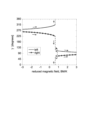
Figure 3: The angle of magnetization $\gamma$ for the left and right electrodes with $\alpha_{R}=-\alpha_{L}=60^{\circ}$, $\beta=90^{\circ}$, and $K/M=38$ mT calculated for the case with biaxial anisotropy. The magnetic field starts from a high negative field and sweeps to positive values.

The results of the numerical simulation are compared to the measured magnetoresistance of a bicrystal sample. The sample is a La_0.7Sr_0.3MnO₃ (LSMO) film grown on a SrTiO₃ bicrystal substrate. The bicrystal is a symmetric (001)-tilt grain boundary with a misorientation angle of $\pm 15^{\circ}$, i.e. the [100] directions of the left and right sides are in-plane rotated $15^{\circ}$ (in opposite directions) with respect to the grain boundary. The 120 nm thick film was grown by pulsed injection metal-organic chemical vapour deposition (MOCVD). More details on the growth procedure can be found in Ref. Dubourdieu et al. (2001). The good epitaxy of the film was verified by x-ray diffraction in $\theta$–$2\theta$- and $\phi$-scans. The out-of-plane lattice parameter of the film was found to be 3.86 Å, to be compared to the bulk pseudo-cubic lattice parameter of the perovskite structured LSMO of 3.88 Å. It is known that this kind of tensile strain leads to an in-plane biaxial magnetocrystalline anisotropy in the $\langle 110\rangle$-directions.Steenbeck and Hiergeist (1999); Berndt et al. (2000) Hence, this LSMO on SrTiO₃ system can be analyzed with the two-dimensional model considered for the Stoner-Wohlfart theory. The saturation magnetization of the film, determined in a superconducting quantum interference device (SQUID) magnetometer, was $400$ kAm^-1.

A 5 $\mu$m wide and about 150 $\mu$m long microbridge crossing the grain boundary was defined by photolithography and Ar-ion milling, and the ends of the microbridge were connected to electrical contacts. The resistance of the grain boundary was measured in a four-contact geometry with a current bias of 10 $\mu$A. The magnetoresistance ($R(B)/R(0)$) was measured with the field applied along the length of the microbridge, i.e. in the plane of the film and perpendicular to the grain boundary. The magnetic field was swept with 0.05 T/min. The dependence of the magnetoresistance on the magnetic field direction is presented in Gun .

The two energy terms in Eq. 1 are comparable in size when the field is $B\approx K/M$. For LSMO films on SrTiO₃ numerical values of $K$ of 1.6 – 5.7$\times 10^{3}$ J/m³ Berndt et al. (2000); Steenbeck and Hiergeist (1999) have previously been reported. In addition we have $M=400$ kAm^-1, as stated above. Hence a simple estimate of the critical field for magnetization switching would give $K/M=$4 – 14 mT.

Since the measured sample has a misorientation angle of $\pm 15^{\circ}$, and the easy axes are in the [110] and equivalent in-plane directions, $\alpha_{L,R}=\pm 60^{\circ}$. The field applied along the microbridge corresponds to $\beta=90^{\circ}$. Using these parameters in Eq. 1 we can fairly well reproduce the measured grain boundary magnetoresistance, see Fig. 4. Here we use a $K/M$ ratio of 38 mT, $P=1$ and $G=20$. Hence, the $K/M$ from the experimental results is within one order of magnitude of the value estimated above.

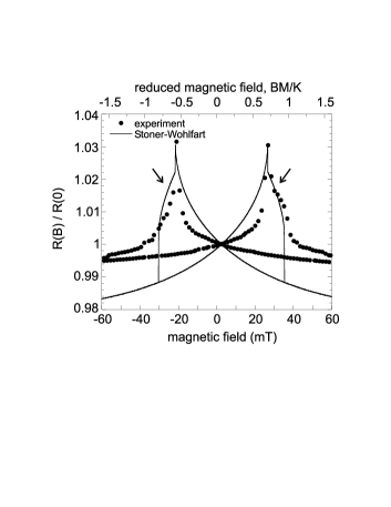
Figure 4: The magnetoresistance of a manganite grain boundary. The circles are measured at 1.9 K according to the descriptions in the text. The solid line is a fit to Eq. 2 with $P=1$ and $G=20$ (using $K/M=38$ mT in Eq. 1). The arrows indicate the shoulder discussed in the text.

The width of the simulated magnetoresistance hysteresis (the distance between the peaks) is uniquely determined by the $K/M$ ratio. The general shape of the curve is determined by the chosen type of magnetocrystalline anisotropy (uniaxial or biaxial) together with the angles of the easy axes ($\alpha_{L}$ and $\alpha_{R}$). The curvature of the magnetoresistance mainly depends on the transport model Not (b). The height of the simulated magnetoresistance depends on the values chosen for $P$ and $G$. It is obvious from Eq. 2 that a decreased spin polarization ($P<1$) has virtually the same effect as an increased non-spinpolarized current ($G>0$). In the simulation we used $P=1$ and $G=20$, but for instance $G=0$ and $P=0.22$ would yield the same magnetoresistance magnitude. Without further information about either $P$ or $G$, a ratio between the two can not be extracted from the measured data with our model.

We note that in the measured curve, there is a peak and a shoulder on each wing of the hysteretic curve. Both these features are represented in the curve (solid line in Fig. 4) calculated from Eq. 2. Each feature is associated with a jump in the magnetization direction. A closer look into the model of biaxial anisotropy reveals that the first jump comes from the switching from a high energy state to one with lower energy, marked I in Fig. 2b. In the low-energy valley there are two local minima. Thus the first part of the magnetization rotation is paused when the first of the two minima is reached in the direction of rotation. However, under some geometrical conditions there exists a state even lower in energy, and the second jump (II) is a transition to that state. The dwelling in the intermediate state creates the shoulder (marked by arrows in Fig. 4) in the magnetoresistance curve. We note that this intermediate state does not exist in the case of uniaxial anisotropy (see Fig. 2a). Thus, we conclude that with the Stoner-Wohlfart model we can well reproduce the characteristic features of the low-field magnetoresistance related to bicrystal grain boundaries, in the case when the magnetic field is perpendicular to the grain boundaries and a biaxial anisotropy is included.

We find the agreement between the numerical values obtained in the model and in experiments to be good, although there are details that are not fully reproduced. In the model, the magnetocrystalline anisotropy $K$ and the magnetization $M$ uniquely determine the position of the peak. Considering the uncertainty in the experimental material parameters the estimated position agrees well with the experiments. By including surface effects at the grain boundary, which may locally decrease $M$ and enhance the effective value of $K$, the agreement can be improved.

Our simulation underestimates the curvature of the magnetoresistance curve. The curvature is determined by the transport model and here we have used the one by Slonczewski Slonczewski (1989), who considered a single-band direct tunneling process. From $I-V$ measurements we know that direct tunneling is insufficient to explain the transport properties in this kind of junctions Klein et al. (1999). We also note that an enhanced curvature has been observed with an increased bias current Westerburg et al. (1999). Hence, our results propose that a more complete transport model for this kind of magnetic tunnel junctions should be developed. Furthermore, the good agreement between the Stoner-Wohlfart model and the shape of the magnetoresistance curves motivates future studies of the electrical transport in this kind of systems.

The presence of the shoulder in the magnetoresistance hysteresis and its relation to the biaxial anisotropy have not, to our knowledge, been explicitly studied previously. García and Alascio García and Alascio (2002) did use a Stoner-Wohlfart-like approach to the problem, but failed to demonstrate the influence of biaxial anisotropy. However, Philipp et al Philipp et al. (2000) and Todd et al Todd et al. (2001) present magnetoresistance curves for single magnetic bicrystal junctions with the field applied perpendicular to the grain boundary, and both curves show a behaviour similar to what can be expected from a coherent rotation of magnetisation direction with biaxial magnetocrystalline anisotropy.

A reason for the shortage of experimental data may be that the shoulder only appears under two conditions: at low temperatures and for a certain range of angular relations between the grain boundary, the anisotropy axes, and the applied magnetic field. In the paper by Gunnarsson et al. Gun , which shows measurements on the same sample as presented here, the shoulder is absent in the magnetoresistance hysteresis measured at 100 K (with the field perpendicular to the grain boundary). One reason for the $T$-dependence is of course the strong variation of the magnetic properties with temperature. It should be noted that the Stoner-Wohlfart model is valid for coherent rotation and thus sufficient to describe the case when the field is applied perpendicular to the grain boundary, in our experimental setup. With the field applied in another direction (e.g. parallel to the grain boundary Gun ) the magnetization reversal processes become more complex. In that case one has to include contributions from the magnetostatic and exchange energy terms in the simulation.

In summary, we proposed that the Stoner-Wohlfart theory can be applied to manganite grain boundary magnetoresistance. Our conclusion is that the model of two magnetically decoupled electrodes with coherently rotating magnetization vectors very well explain the experimental data. We find that in the case of La_0.7Sr_0.3MnO₃ junctions on SrTiO₃ bicrystals it is necessary to include a biaxial magnetocrystalline anisotropy to fully reproduce the measured data. In addition our study shows that a bicrystal grain boundary, with its well defined angles of magnetization, constitutes a system well designed to explore the physics of magnetic tunnel junctions.