Optical spectral weight distribution in -wave superconductors
Abstract
The distribution in frequency of optical spectral weight remaining under the real part of the optical conductivity in the superconducting state of a -wave superconductor depends on impurity concentration, on the strength of the impurity potential as well as on temperature and there is some residual absorption even at . In BCS theory the important weight is confined to the microwave region if the scattering is sufficiently weak. In an Eliashberg formulation substantial additional weight is to be found in the incoherent, boson assisted background which falls in the infrared and is not significantly depleted by the formation of the condensate, although it is shifted as a result of the opening of a superconducting gap.
pacs:
74.20.Mn 74.25.Gz 74.72.-hI Introduction
When a metal enters its superconducting state, optical spectral weight is lost at finite frequencies under the real part of the optical conductivity, .mars1 Provided the change in kinetic energy between normal and superconducting state is small and can be neglected, the missing spectral weight reappears as a contribution at zero frequency which originates in the superfluid, and the over all optical sum rule of Ferrell, Glover, and Tinkhamferrell ; tinkham remains unchanged. The distribution in frequency of the remaining spectral weight under depends on gap symmetry, on the nature of the inelastic scattering involved, on the concentration and scattering strength of the impurities, and on temperature.vM In this paper we consider explicitely the case of -wave gap symmetry within a generalized Eliashberg formalism.schach8 In this approach the optical conductivity (as well as the quasiparticle spectral density) contains an incoherent part associated with boson assisted absorption which is not centered about zero frequency and which contributes to the optical spectral weight in the infrared range. In addition there is the usual quasiparticle contribution of BCS theory. Alternate approaches to include inelastic scattering exist. In several works, the quasiparticle scattering rate due to coupling to spin fluctuations is simply added to a BCS formalism through an additional scattering channel.quinla ; hirschf ; quinlb ; hirschf1 Nevertheless, whenever we refer to BCS within this paper we mean the standard theory without these additional features.
In BCS theory the London penetration depthBCS6 ; carb at zero temperature in the clean limit is given by ( is the free electron density, is the charge on the electron, is its mass, is the plasma frequency, and we have set the velocity of light equal to 1) and all the optical spectral weight condenses. However, as the impurity mean free path is reduced, not all the spectral weight is transferred to the condensatetanner ; liu and there remains some residual impurity induced absorption.turner ; corson ; resabs Details depend on gap symmetry.
In Eliashberg theory the pairing interaction is described by an electron-phonon spectral density, denoted by .BCS6 ; carb ; no7 Twice the first inverse moment of , gives the quasiparticle mass renormalization with the effective to bare mass ratio . While the gap and renormalization function of Eliashberg theory acquire a frequency dependence which requires numerical treatment, a useful, although not exact, approximation is to assume that the important frequencies in are much higher than the superconducting energy scale and, thus, one can approximate the renormalizations by a constant value.carb In this approximation, the zero temperature penetration depth is in the clean limit. Thus, the electron-phonon renormalization simply changes the bare mass in the London expression to the renormalized mass . This result does not depend explicitly on the gap and holds independent of its symmetry. A naive interpretation of this result is that only the coherent quasiparticle part of the electron-spectral density [which contains approximately of the total spectral weight of one] condenses. While this is approximately true, we will see that the incoherent part which contains the remaining part of the spectral weight is also involved, although in a more minor and subtle way.
In an -wave superconductor the entire incoherent part of the conductivity is shifted upward by twice the gap value, , when compared to its normal state. It is also slightly distorted but, to a good approximation, it remains unchanged. The fact that there is a shift between normal and superconducting state implies that an optical spectral weight shift originates from this contribution even if its overall contribution to the sum rule should remain the same. For a -wave superconductor the situation is more complex because the gap is anisotropic and, thus, the shift by varies with the polar angle on the two-dimensional Fermi surface of the CuO2 planes.
The goal of this paper is to understand, within an Eliashberg formalism, how the remaining area under the real part of the optical conductivity is distributed in frequency, how this distribution is changed by finite temperature effects and by the introduction of elastic impurity scattering, and what information can be obtained from such studies about the superconducting state and the nature of the mechanism which drives it.
In reference to -wave superconductivity in the cuprates two boson exchange models which have received much attention are the Nearly Antiferromagnetic Fermi Liquid (NAFFL) modelpines1 ; pines2 ; schach4 ; schach5 ; schach7 ; schach6 and the Marginal Fermi Liquid (MFL) model.varma1 ; varma2 ; varma3 Both models are characterized by an appropriate charge carrier-exchange boson spectral density which replaces the of the phonon caseBCS6 ; mcmillan ; mcmillan1 ; mars4 and which reflects the nature of the inelastic scattering envisioned. In the NAFFL model a further complication arises in that we would expect to be very anisotropic as a function of momentum on the Fermi surface. For simplicity we ignore this complication here. Also, in principle, a different spectral weight function can enter the gap and renormalization channel, respectively.
In Section II, we provide some theoretical background. The quasiparticle spectral density as a function of energy is considered as is the effect of impurities on it. In Sec. III we give the necessary formulas for the optical conductivity and discuss some results. In Sec. IV the conditions under which a partial sum rule involving only the quasiparticle part of the spectral density can be expected are described. Section V deals with issues associated with the residual absorption and Sec. VI deals with a more detailed discussion of optical spectral weight readjustment due to superconductivity. Conclusions are found in Sec. VII.
II Quasiparticle spectral density
We begin with a discussion of the quasiparticle spectral density which will allow us to understand the basic features expected of the optical conductivity. In Nambu notation the -matrix Green’s function in the superconducting state is given in terms of the single quasiparticle dispersion with momentum k, the renormalized Matsubara frequency and the pairing energy which for a -wave superconductor is proportional to . In terms of Pauli’s matrices
| (1) |
The quasiparticle spectral density is given by
| (2) | |||||
The generalized Eliashberg equations applicable to -wave gap symmetry which include renormalization effects in the -channel have been written down before and will not be repeated here.schach8 They are a set of coupled non-linear integral equations for and which depend on an electron-boson spectral density . The boson exchange mechanism involved in superconductivity is what determines its shape in frequency and its magnitude. In general, the projection of the electron-boson interaction on the and -channel can be different but for simplicity, here, the same form of is used in both channels but with a different magnitude: we use with for the -channel.
In Fig. 1 we present numerical results for based on numerical

solutions of the Eliashberg equations. The kernel used for the numerical work is shown in the inset in the top frame of Fig. 2 and was obtained from consideration of the infrared optical conductivity of YBa2Cu3O6.95 (YBCO6.95).schach7 Besides coupling to an optical resonance at meV (the energy where a spin resonance is also seen in the inelastic neutron scatteringbourges ) which grows with decreasing temperature into the superconducting state, there is also additional coupling to a broad spin fluctuation spectrum background of the form introduced by Millis et al.pines1 in their NAFFL model. This is seen as the long tail in which extends to very high energies of order meV. The existence of these tails is a universal property of the cuprates.tanner ; liu ; schach6 ; puchkov ; homes ; tu This energy scale is of the order of the magnetic parameter in the model.sorella A flat background spectrum is also characteristic of the MFL model.varma1 ; varma2 ; varma3 In this work, the shape and size of is fixed from our previous fit to optical dataschach7 and left unchanged. It applies at low temperatures in the superconducting state (K).
The top frame of Fig. 1 gives results for the charge carrier spectral density vs where implies that we consider only the Fermi energy in Eq. (2). The results are for a pure sample with meV and . Here, is proportional to the impurity concentration and is related to the normal state impurity scattering rate equal to , where . is the normal state density of states at the Fermi energy and the strength of the impurity potential. These impurity parameters were determined to fit well the microwave data in YBCO6.99 obtained by Hosseini et al.hoss The solid curve is for the nodal direction and the dashed curve for the antinodal direction. The spectral gap is the value of evaluated at the frequency of the coherence peak in the density of states
| (3) | |||||
and is equal to meV. This is also the position of the large peak seen in the dashed curve in the top frame of Fig. 1. However, there is no gap in the nodal direction, and in this case the spectral function is peaked about . It rapidly decays to nearly zero within a very narrow frequency range determined by a combination of the small impurity scattering rate which we have included and the equally small inelastic scattering which reflects the presence of and finite temperature. A second peak is also observed at higher energies but with reduced amplitude. This peak has its origin in the incoherent boson assisted processes described by the spectral density . Note that the two contributions are well separated. In the constant model, the coherent part
| (4) |
is a Lorentzian of width and has total weight of . The remaining weight in the complete spectral density which is normalized to one, is thus to be found in the incoherent, boson assisted background. Returning to the antinodal direction, we see that in this case the separation between quasiparticle peak and incoherent boson assisted background is lost as the two contributions overlap significantly. In the bottom frame of Fig. 1 we show similar results for the charge carrier spectral density but now a larger amount of impurity scattering is included with meV (Ref. schach2, ) and the unitary limit is taken, i.e. . In this instance, even for the nodal direction, impurities have the effect of filling in the region between quasiparticle and incoherent background (solid curve). Also for the antinodal direction (dashed curve), because we are in -wave, the region below the gap energy which is now meV is filled in significantly. It would be zero in BCS -wave. At , and in antinodal direction
| (5) |
which is finite. Here is the quasiparticle scattering rate at zero frequency in the superconducting state. It is calculated in Sec. V. This limit is not universal in contrast to the universal limit found by Leelee for the real part of the electrical conductivity at zero temperature which is in the constant model. Note that what enters the universal limit is the renormalized mass rather than the bare mass. This important fact has generally been overlooked in the discussion of this limit even though the difference can be numerically large (order ). We note one technical point about our Eliashberg numerical solutions. In all cases is kept fixed as is K. In a -wave superconductor the introduction of impurities, of course, reduces the critical temperature. What is done is that the parameter which multiplies in the gap channel is readjusted slightly to keep fixed. This procedure leads to the larger value of the spectral gap seen in the bottom frame of Fig. 1 as compared with the top frame (dashed lines).
III Infrared conductivity
A general expression for the infrared optical conductivity at temperature in a BCS -wave superconductor isschach1 ; schach2 ; schur
| (6) |
where the function takes on the form
| (7) | |||||
In Eq. (6) , with the Boltzmann factor. In Eq. (7)
| (8a) | |||
| and | |||
| (8b) | |||
and , , and are the complex conjugates of , , and , respectively. These expressions hold for an Eliashberg superconductor as well as for BCS in which case the gap does not depend on frequency; it only depends on temperature, and on angle. Here, for brevity we have suppressed these dependencies but they are implicitly implied by the brackets in Eq. (6) which denote an angular average over momentum directions of electrons on the Fermi surface at a given temperature.
Figure 2 presents two fits of theoretical results to experimental data for the real part of the optical conductivity

. The top frame presents a comparison with data reported by Homes et al.homes for an untwinned, optimally doped YBCO6.95 single crystal (solid line) at K. The dashed line corresponds to the best fit theoretical results generated using extended Eliashberg theory. The phenomenologically determined electron-boson spectrum reported by Schachinger et al.schach7 (shown in the inset) was used. The impurity parameters meV and resulted in this best fit.schach2 For comparison the dotted line corresponds to the results of a BCS calculation using the same impurity parameters. It is obvious that the BCS calculation cannot reproduce the boson assisted higher energy incoherent background which starts at about meV. The full Eliashberg theory, on the other hand, is capable of modeling very well the experimental data over the whole infrared region. The bottom frame of Fig. 2 shows restricted to the microwave region up to meV. Three temperatures are considered, namely K (solid curve), K (dashed curve), and K (dotted curve). The impurity parameters were varied to get a good fit to the data of a high purity YBCO6.99 sample reported by Hosseini et al.hoss and presented by symbols. The best fit was found for meV and . It is clear that this sample is very pure and that it is not in the unitary limit. All curves for vs in this frame show the upward curvature characteristic of finite values. Unitary scattering would give a downward curvature in disagreement with the data.
The excellent agreement between theory and experiment shown in Fig. 2 encourages us to apply theory to discuss in detail, issues connected with the redistribution of optical spectral weight in going from the normal (not always available in experiment) to the superconducting state and the effect of temperature and impurities on it.
The real part of the optical conductivity as a function of is shown in the top frame of Fig. 3. A factor has been omitted from all theoretical calculations and so is in meV-1. In these units the usual FGT sum rule which gives the total available optical spectral weight (including the superfluid contribution at ). Two cases are shown in the frequency range meV. One is for the very pure sample (solid curve) with meV and . The other is for a less pure sample (dotted curve) with meV in the unitary limit, . In the solid curve we clearly see a separate quasiparticle contribution peaked about which is responsible for a coherent Drude like contribution to the real part of the optical conductivity. In this process the energy of the photon is transferred to the electrons with the impurities providing a momentum sink. The width of the quasiparticle peak and corresponding Drude peak is related to the impurity scattering rate. Because we are using Eliashberg theory there is also a small contribution to this width coming from the thermal population of excited spin fluctuations. In addition, there is a separate incoherent contribution at higher frequencies. This second contribution involves the creation of spin fluctuations during the absorption process. Its shape reflects details of the frequency dependence of the spectral density involved. For the normal state at temperature the spectral density in the NAFFL model does not show the resonance peak seen in the insert of the top frame of Fig. 2 but consists mainly of the reasonably flat background. This implies that in this region MFL behavior results with optical and quasiparticle lifetimes linear in frequency and in temperature. The energy scale associated with this behavior is the spin fluctuation scale . This is verified in numerous experiments in the cuprates as reviewed by Puchkov et al.puchkov Just as for the charge carrier spectral density discussed in the previous section, the optical weight under the

coherent part, to which we add the superfluid contribution at , is about of the total weight available with the remainder, , to be found in the incoherent part. In the model considered here, which fits the available data for YBCO6.99 and YBCO6.95, so that only one third of the weight is in the coherent part. This order of magnitude agrees well with the extensive experimental results in other cuprates given in Refs. tanner, ; liu, . Note that coherent and incoherent region are nicely separated over a substantial frequency range in which the conductivity is small relative to its value in the quasiparticle peak and in the boson assisted background. This will lead to a plateau in the integrated optical spectral weight as a function of the upper limit in the integral over which will in turn lead to an approximate partial or truncated sum rule on the coherent contribution to the conductivity itself. It is only this piece which is included in BCS theory and which can be described by such a theory in cases when it is well separated from the incoherent background. We note that the addition of impurities, as in the dashed curve in the top frame of Fig. 3, greatly increases the frequency width of the quasiparticle peak in and also fills in the region between coherent and incoherent part of the conductivity. While these two contributions are still recognizable as distinct, they now overlap significantly and cannot as easily be separated.
Finally, but very importantly, in the bottom frame of Fig. 3 we repeat the curve for vs for the pure sample of the top frame of Fig. 3 (solid curve) and compare it with its normal state counterpart (dotted curve). We see that due to superconductivity, much of the weight under the Drude peak in the solid curve (superconducting) as compared with the dotted curve (normal) has been transferred to the condensate and is not part of the figure [-function at in ]. It has also shifted the incoherent part to higher energies. For an -wave superconductor the appropriate shift would be twice the gap as seen in the work of Marsiglio and Carbottemars1 (see their Fig. 11). For the -wave case there is a distribution of gap values around the Fermi surface and consequently of upward shifts. This leads to some distortion of the incoherent part as compared with its normal state value as can be seen in the dashed curve which is the dotted curve displaced upwards by meV, a value slightly larger than the gap of meV and much less than twice the spectral gap. The difference between dashed and solid curve is small but not negligible. This shows that in the optical spectral weight distribution the boson assisted part of the spectrum is in a first approximation shifted in energy but not significantly depleted or augmented. The addition of impurities also have an effect on the incoherent background as can be seen in the top frame of Fig. 3 on comparison of the solid with the dashed curve.
IV Approximate Partial sum rule for the coherent part
In the top frame of Fig. 4 we show our theoretical

results for the remaining integrated optical spectral weight under the real part of the conductivity in the superconducting state up to frequency . By definition where the upper limit of the integral is variable. The data is for the very pure sample for which coherent and incoherent contributions are well separated. Results for three temperatures are shown, namely K (solid line), K (dashed line), and K (dotted line) and the variable upper limit ranges from zero to meV, i.e. only very low frequencies are sampled, consequently only the coherent quasiparticle contribution to the conductivity (solid curve in the top frame of Fig. 2) is significantly involved since the incoherent contribution is almost negligible in this energy range. Note that already for meV a well developed plateau is seen in each curve, although its magnitude depends on temperature. represents the residual absorption in the microwave region that remains at low temperatures in the superconducting state. It decreases with decreasing temperature as more optical weight is transferred to the condensate. In our calculations this residual absorption has its origin in the inelastic scattering associated with thermally activated bosons which exist at any finite and which broadens the quasiparticle contribution. This is in addition to impurity absorption which is also small, when is small. Strictly, at zero temperature only the impurity absorption remains and this goes to zero as goes to zero. We will see later that an extrapolation to zero temperature of the numerical data for gives for the cut off meV, a value of 0.00023 [in units of ] which is very small.
In the bottom frame of Fig. 4 we show results for a closely related quantity vs in units of . In the superconducting state, missing spectral weight under the real part of the conductivity when compared to its normal state is found in a delta-function at weighted by the amount in the condensate. In our computer units the full sum rule which applies when is integrated to infinity and the condensate contribution added, is two. The partial sum up to is
| (9) | |||||
and is shown for the same three temperatures as in the top frame. Here is the imaginary part of the conductivity. When multiplied by its limit is proportional to the inverse square of the London penetration depth which, in turn, is proportional to the superfluid density.
For an Eliashberg superconductor the expression for the penetration depth at any temperature is (in our computer units)
| (10) |
For in the constant model with no impurities we get
| (11) | |||||
where we have restored the units and is the usual value of the London penetration depth. There are so called strong coupling corrections to Eq. (11) (see Ref. carb, ) but these are small and, in a first approximation, can be neglected. A physical interpretation of Eq. (11) is that it is only the coherent quasiparticle part of the spectral density (Fig. 1) which significantly participates in the condensation.
Returning to the bottom frame of Fig. 4 we see that at meV a plateau has been reached in vs as well and that, relative to what is the case for in the top frame, little variation with temperature remains. Nevertheless, the small amount that is seen will have consequences as we will describe later. For now, neglecting this -dependence, the plateau seen in vs implies that an approximate partial sum rule will apply to the coherent part of the conductivity by itself, provided the cut off on is kept small. This has important implications for the analysis of experiments. While only approximately of the optical spectral weight is involved in this contribution, this piece behaves like a BCS superconductor. The partial sum rule which applies, when the cut off is kept below the frequency at which the incoherent part starts to make an important contribution is
| (12) |
in the constant approximation of Sec. II. In our full Eliashberg calculations for K we get for Eq. (12) instead of with . It is the existence of the partial sum rule (12) for very pure samples that has allowed Turner et al.turner to analyze their microwave data within a BCS formalism without reference to the mid infrared incoherent contribution. Nevertheless, one has to keep in mind that this partial sum rule involves only of the whole spectral weight under the curve with important consequences on the results derived from such an analysis.
For the pure case considered here the cutoff in (12) is well defined. This is further illustrated in Fig. 5 where we

show once more (top frame) and (bottom frame) but now for an extended frequency range up to meV for the case K only. We also show, for comparison, additional BCS results and results for a second set of impurity parameters. The solid and dotted curves in both frames are and for an Eliashberg superconductor with meV, and meV, , respectively. The dashed and dash-dotted curves are for a BCS superconductor with meV, and meV, . We first note that for the purer Eliashberg case (dotted curve) the plateau in both, and identified in Fig. 4 extends to meV. Clearly, any value of frequency between meV and meV will do for in Eq. (12) and a partial sum rule is well defined but for the less pure case (solid curve) a plateau is not as well defined. In both cases, however, the increase beyond the plateau value of towards saturation is rather slow and even at meV is still well below 2. This feature reflects directly the large energy scale involved in the boson exchange mechanism we have used. This behavior is in sharp contrast to BCS. For the dash-dotted curve is already close to two at meV while for the less pure case (dashed curve) the rise to two is slower and distributed over a larger energy scale of the order meV. In as much as impurities strongly affect such scale estimates they are not fundamental to the superconductivity itself. If, in our Eliashberg calculations, we look only at the initial rise to its plateau value , the scales involved are different again, meV and meV respectively.
V Relation between residual absorption and penetration depth
We next turn to the relationship between the temperature dependence of the residual absorption and the penetration depth. This is illustrated in Fig. 6 which has three frames. The top frame presents BCS results and is for comparison with the two

other frames which are based on Eliashberg solutions. The central frame has impurity parameters meV and . The bottom frame is for a less pure sample with meV and and illustrates how impurities change the results. In the top frame, the dashed curve is the difference in superfluid density as a function of temperature up to K for a BCS superconductor with gap meV, meV, and . These parameters were chosen only for the purpose of illustration. Turner et al.turner considered the optical spectral weight concentrated in the microwave region of an ortho-II YBCO6.5 sample and the temperature dependence of that is obtained from consideration of the microwave region only. They found it to extrapolate to a finite value at (zero temperature residual absorption) while at the same time parallels the temperature dependence found for the penetration depth. In our solid curve (top frame of Fig. 6 we have integrated to get up to meV and find a curve for which is parallel to the dashed curve for the penetration depth but indeed does not extrapolate to zero at . Note that in a BCS model for pure samples the ordinary FGT sum rule applies even if only the microwave region is considered and so the solid and dashed curves are parallel. This is no longer the case in Eliashberg theory as shown in the center frame of Fig. 6. There the dashed and solid curves are not quite parallel with the dashed curve showing a slightly steeper slope. Also, the solid curve extrapolates to a finite though very small value at . This is expected since the impurity content in this run is very small. This case corresponds closely to the YBCO6.99 sample considered in Fig. 4 of Turner et al.turner The slight difference in slope between solid and dashed curve can be understood in terms of our result for given in the bottom frame of Fig. 4. We have already noted that at meV, the cutoff used in evaluation of (solid curve, center frame of Fig. 6) there remains a small temperature dependence to the saturated value of . This means that in this region is slightly smaller at K (dotted curve in the bottom frame of Fig. 4) than it is at K (solid curve). This slight deviation from the partial sum rule embodied in our Eq. (12) leads immediately to the difference in slope seen in the center frame of Fig. 6 between and the penetration depth.
In the bottom frame of Fig. 6 we show results for meV and . In this case the coherent and incoherent contribution to (see Fig. 3, top frame, dotted curve although this curve is for ) are not as well separated as in the pure case and vs does not show as clear a plateau which would allow the formulation of a partial sum rule on the coherent part alone. Nevertheless, we do note that for meV, (solid squares) is nearly parallel to the dashed curve for the penetration depth. If, however, is increased to meV (solid up-triangles), or meV (solid down-triangles) this no longer holds. This result can be traced to the fact that no real temperature and cut off independent plateau is reached in these cases. Thus, there is no partial sum rule which can be applied on and an analysis as performed by Turner et al.turner on very high purity samples appears not to be possible. This case may correspond better to the relatively dirtier film data.corson Note in particular, the residual absorption at zero temperature depends now strongly on the cutoff frequency chosen for the partial sum rule. In our example (bottom frame of Fig. 6) the residual absorption increases almost linearly with increasing cutoff frequency.
We turn next to the zero temperature value of the residual absorption and its impurity dependence. Eq. (10) applies but now we wish to consider impurities so that is not simply in the constant model. Instead, we must use
| (13) |
which needs to be solved self consistently for . For , we can write with
| (14) |
and is given by Eq. (3). Evaluating gives
| (15) |
This transcendental equation for , the zero frequency scattering rate at zero frequency, is to be solved numerically for any value of . Results can be found in Refs. schach2, and schach1, for the case . What is found is that increases with and, for a given value of decreases rapidly with . At we get the approximate, but very useful relation
| (16) |
Note, this is the same expression as in Hirschfeld and Goldenfeldhirschf2 except that it contains an additional factor of . In terms of we can get an approximate expression for the zero temperature London penetration depth including impurities. Returning to Eq. (10) we need to replace by to getschach1
| (17) | |||||
| (18) |
where is the elliptic integral of the first kind. The approximation made to get the last equality, Eq. (18), is not very accurate but has the the important advantage that it is analytic and simple. It gives
| (19) |
In a BCS model this gives in the limits and
| (20) | |||||
Exact numerical results for based on Eq. (17)
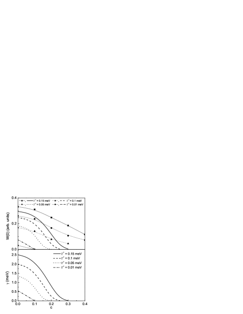
with are compared with those based on Eq. (20) in the top frame of Fig. 7. We see that Eq. (20) is qualitatively but not quantitatively correct. In the bottom frame we show the corresponding values of vs for the convenience of the reader. It is clear that the residual absorption due to the coherent part of the charge carrier spectral density does depend significantly on impurity content. In a real superconductor we have additional absorption at coming from the incoherent, boson assisted background which enters when in the upper limit of the defining integral for is made to span energies in the infrared region of the spectrum.
VI Missing area
The FGT sum rule implies that the missing optical spectral weight under the real part of the conductivity in the superconducting state appears as a delta function contribution at the origin proportional to the superfluid density. It depends on temperature and on impurity content. Increasing and/or decreases the superfluid density. In the top frame of Fig. 8 we show

our results for the remaining integrated optical spectral weight as a function of up to meV for a sample with meV and . We have done similar calculations for a clean sample but there is no qualitative difference. The solid curve is for the superconducting state at K and is to be compared with the dotted curve which is for the normal state at the same temperature. We see a great deal of missing spectral weight between these two curves with rising much faster at small than and it is rising to a much higher value. The difference (dashed curve) is the amount of optical spectral weight between that has been transferred to the superfluid condensate. As we see, the dashed curve rapidly grows within a few meV to a value close (but not quite) to the asymptotic value it assumes at meV. After this the remaining variation is small but there is a shallow minimum around meV with a corresponding broad and slight peak around meV which is followed by a small gradual decrease still seen at meV. These features can be understood in detail when the frequency dependence of is considered. The relevant curves to be compared are the dotted (normal) and solid (superconducting) in the bottom frame of Fig. 8. Both are at K. The curves cross at 3 places on the frequency axis. Above the first crossing at meV the difference in the integrated area decreases till meV at which it begins to increase. Finally, at the third crossing meV it begins to decrease again towards its value at meV. These features are the direct result of the shift in incoherent background towards higher energies due to the opening up of the superconducting gap. The area between the dotted and solid lines that falls between and is made up slowly at higher frequencies. This feature would not be part of BCS theory in which case the energy scale for the optical weight which significantly participates in the condensate is set as a few times the gap dolgov and the saturated value is reached from below rather than from above. In our theory the existence of the incoherent background effectively increases this scale to much higher energies, the scale set by the bosons involved, although the amount of spectral weight involved is very small.homes1 ; sant We note that at meV the missing area curves and of the top frame of Fig. 8 are still about 2.5% higher than the value indicated for the penetration depth (thin dash-double dotted line) which is obtained directly from the imaginary part of the optical conductivity.
In an actual experiment it is not possible to access the normal state at low temperatures so that cannot be used to compute the difference with . Usually is used instead. This is shown as the dashed-double dotted curve in the top frame of Fig. 8 which is seen to merge with the dotted curve only at large values of . Because in our theoretical work, the inelastic scattering at is large with a scattering rate of the order or so, the corresponding optical spectral weight in is shifted to higher energies. Consequently, rises much more slowly out of than does and the difference curve (dash-dotted curve) reflects this. It merges with the dashed curve only for meV. Thus, making use of rather than makes a considerable difference in the estimate of the dependence of the missing area. None of the structure seen in the dashed curve remains in the dash-dotted curve and much information on separate coherent and incoherent contributions is lost, although the curve still approaches its limiting value from above. From this point of view, it is the dashed curve which is fundamental but it is not directly available in experiments. If an even higher temperature had been used for the normal state, say around room temperature, the frequency at which the difference would agree with the penetration depth is pushed to very high energies well beyond the meV range shown in the top frame of Fig. 8. The reason for this is clear when the bottom frame of this same figure is considered. What is shown is the real part of the conductivity for four cases: the normal state at K (dashed curve), at K (dash-dotted curve), and at K (dotted curve). Increasing the normal state temperature shifts a lot of spectral weight to higher energies and can even make the difference negative for small .
We stress again that individual curves show no saturation as a function of in the range shown. This is characteristic of the high oxides and resides in the fact that , the electron-boson exchange spectral density, extends to very high energies. This is fundamental to an understanding of the optical properties in these materials and is very different from the electron-phonon case. In that instance there is a maximum phonon energy never larger than about meV and hence the curve for would reach saturation at a much smaller energy than in our work. This observation provides strong evidence against solely a phonon mechanism for superconductivity in the oxides.
To aid this discussion we added Fig. 9 which, in its top frame, shows the experimental data for the real part of the optical conductivity, reported by Tu et al.tu in an optimally doped Bi2Sr2Ca Cu2O8+δ (Bi2212) single crystal for three temperatures, namely,

, , K. The experimental data has been augmented by theoretical dataschach8 in the frequency region meV derived from best fits to experiment. This graph is to be compared with the bottom frame of Fig. 8. The bottom frame of Fig. 9 presents the corresponding optical spectral weight calculated from the experimental data. The results follow closely similar theoretical curves presented in the top frame of Fig. 8. In particular, K) does not develop a well defined plateau around meV as we found it for optimally doped YBCO6.95 single crystals [solid line in the top frame of Fig. 8, labeled K]. Finally, the differences (solid line) and (dash-double dotted line) are shown in this graph. We also included the theoretical value for as a thin, solid horizontal line found from a fit to experimental data. The first difference is still far away from this limit but approaches it from above, as expected from our previous discussion, while the second approaches this limit from below. This analysis of experimental data supports our theoretical results in a rather impressive way.
VII Conclusions
In a pure BCS superconductor at zero temperature with no impurities the entire optical spectral weight under the real part of the conductivity will vanish as it is all transferred to the superfluid density which contributes a -function at to the real part of . When impurities are present the superfluid density at is reduced from its clean limit value and some spectral weight remains under which implies some absorption even at zero temperature. The situation is quite different for a superconductor which shows a pronounced incoherent background scattering which can be modeled reasonably well in Eliashberg theory be it - or -wave. In both cases it is mainly the coherent part of the electron spectral density which contributes to the condensate. The electron spectral function still has a -function part broadened by the interactions at any finite energy away from the Fermi energy but the amount of weight under this part is , where is the mass enhancement parameter for the electron-boson exchange interaction. The remaining spectral weight is to be found in incoherent, boson assisted tails. Another way of putting this is that at zero temperature in a pure system the superfluid density is related to the renormalized plasma frequency with replacing the bare electron mass in contrast to the total plasma frequency which involves the bare mass . The incoherent, boson assisted tails in do not contribute much to the condensate and in fact remain pretty well unaffected in shape and optical weight by the transition to the superconducting state but they are shifted upwards due to the opening up of the superconducting gap. This shift implies that when one considers the missing optical spectral weight under the conductivity which enters the condensate, the energy scale for this readjustment is not set by the gap scale but rather by the scale of the maximum exchanged boson energy. Also it is expected that the value of the penetration depth which corresponds to the saturated value of the missing area is approached from above when the conductivity is integrated to high energies.
Acknowledgment
Research supported by the Natural Sciences and Engineering Research Council of Canada (NSERC) and by the Canadian Institute for Advanced Research (CIAR). J.P.C. thanks D.M. Broun for discussions. The authors are grateful to Drs. C.C. Homes and J.J. Tu for providing their original experimental data for analysis.
References
- (1) F. Marsiglio and J.P. Carbotte, Aust. J. Phys. 50, 975 (1997), and 50, 1011 (1997).
- (2) R.A. Ferrell and R.E. Glover, Phys. Rev. 109, 1398 (1958).
- (3) M. Tinkham and R.B. Ferrell, Phys. Rev. Lett. 2, 331 (1959).
- (4) H.J.A. Molegraaf, C. Presura, D. van der Marel, P.H. Kes, and M. Li, Science 295, 2239 (2002).
- (5) E. Schachinger and J.P. Carbotte, J. Phys. Studies (L’viv, Ukraine) 7, 209 (2003); E. Schachinger and J.P. Carbotte, in: Models and Methods of High-TC Superconductivity: some Frontal Aspects, Vol. II, ed.: J.K. Srivastava and S.M. Rao, Nova Science, Hauppauge NY (2003), pp. 73.
- (6) S.M. Quinlan, P.J. Hirschfeld, and D.J. Scalapino, Phys. Rev. B53, 8575 (1996).
- (7) P.J. Hirschfeld, S.M. Quinlan, and D.J. Scalapino, Phys. Rev. B55, 12 742 (1997).
- (8) S.M. Quinlan, D.J. Scalapino,and N. Bulut, Phys. Rev. B49, 1470 (1994).
- (9) P.J. Hirschfeld, W.O. Putikka, and D.J. Scalapino, Phys. Rev. B50, 10250 (1994).
- (10) F. Marsiglio and J.P. Carbotte, in Handbook on Superconductivity: Conventional and Unconventional, eds. K.H. Bennemann and J.B. Ketterson (Springer, Berlin, 2003), pp. 233-345.
- (11) J.P. Carbotte, Rev. Mod. Phys. 62, 1027 (1990).
- (12) D.B. Tanner, H.L. Liu et al., Physica B 244, 1 (1998).
- (13) H.L. Liu, N.A. Quijada, et al., J. Phys.: Condens. Matter 11, 239 (1999).
- (14) P.J. Turner, R. Harris, S. Kamal, M.E. Hayden, D.M. Broun, D.C. Morgan, A. Hosseini, P. Dosanjh, G. Mullins, J.S. Preston, R. Liang, D.A. Bonn, and W.N. Hardy, Phys. Rev. Lett. 90, 237005 (2003).
- (15) J. Corson, J. Orenstein, Seongshik Oh, J. O’Donnell, and J.N. Eckstein, Phys. Rev. Lett. 85, 2569 (2000).
- (16) E. Schachinger and J.P. Carbotte, Phys. Rev. B67, 134509 (2003).
- (17) G. Grimvall, The Electron-Phonon Interaction in Metals, (North-Holland, New York, 1981).
- (18) A. Millis, H. Monien, and D. Pines, Phys. Rev. B42, 167 (1990).
- (19) P. Monthoux and D. Pines, Phys. Rev. B47, 6069 (1993); Phys. Rev. B49, 4261 (1994); Phys. Rev. B50, 16015 (1994).
- (20) J.P. Carbotte, E. Schachinger, and D.N. Basov, Nature (London) 401, 354 (1999).
- (21) E. Schachinger and J.P. Carbotte, Phys. Rev. B62, 9054 (2000).
- (22) E. Schachinger, J.P. Carbotte, and D.N. Basov, Europhys. Lett. 54, 380 (2001).
- (23) E. Schachinger and J.P. Carbotte, Physica C 364, 13 (2001).
- (24) C.M. Varma, Int. J. Mod. Phys. 3, 2083 (1989).
- (25) P.B. Littlewood, C.M. Varma, S. Schmitt-Rink, and E. Abrahams, Phys. Rev. B39, 12371 (1989).
- (26) C.M. Varma, P.B. Littlewood, S. Schmitt-Rink, E. Abrahams, and A.E. Ruckenstein, Phys. Rev. Lett. 63, 1996 (1989); ibid. 64, 497 (1990).
- (27) W.L. McMillan and J.M. Rowell, Phys. Rev. Lett. 19, 108 (1965).
- (28) W.L. McMillan and J.M. Rowell, in Superconductivity, ed. R.D. Parks (Marcel Dekker Inc., New York, 1969), p. 561.
- (29) F. Marsiglio, T. Startseva, and J.P. Carbotte, Phys. Lett. A 245, 172 (1998).
- (30) Ph. Bourges, Y. Sidis, H.F. Fong, B. Keimer, L.P. Regnault, J. Bossy, A.S. Ivanov, D.L. Lilius, and I.A. Aksay, in High Temperature Superconductivity, eds. S.E. Barnes, et al., CP483 (American Institute of Physics, Amsterdam, 1999), p. 207.
- (31) A.V. Puchkov, D.N. Basov, and T. Timusk, J. Phys.: Condens. Matter 8, 10049 (1996).
- (32) C.C. Homes, D.A. Bonn, R. Liang, W.N. Hardy, D.N. Basov, T. Timusk, and B.P. Clayman, Phys. Rev. B60, 9782 (1999).
- (33) J.J. Tu, C.C. Homes, G.D. Gu, D.N. Basov, and M. Strongin, Phys. Rev. B66, 144514 (2002).
- (34) S. Sorella, G.B. Martins, F. Becca, C. Gazza, L. Capriotti, A. Parola, and E. Dagotto, Phys. Rev. Lett. 88, 117002 (2002).
- (35) A. Hosseini, R. Harris, S. Kamal, P. Dosanjh, J. Preston, R. Liang, W.N. Hardy, and D.A. Bonn, Phys. Rev. B60, 1349 (1999).
- (36) E. Schachinger and J.P. Carbotte, Phys. Rev. B64, 094501 (2001).
- (37) P.A. Lee, Phys. Lett. 71, 1887 (1993).
- (38) E. Schachinger and J.P. Carbotte, Phys. Rev. B65, 064514 (2002).
- (39) I. Schürrer, E. Schachinger, and J.P. Carbotte, Physica C 303, 287 (1998); J. Low Temp. Phys. 115, 251 (1999).
- (40) P.J. Hirschfeld and N. Goldenfeld, Phys. Rev. B48, 4219 (1993).
- (41) A.E. Karakozov, E.G. Maksimov, and O.V. Dolgov, Solid State Commun. 124, 119 (2002).
- (42) C.C. Homes, S.V. Dordevis, D.A. Bonn, R. Liang, and W.N. Hardy, cond-mat/0303506 (unpublished).
- (43) A.F. Santander-Syro, R.P.M.S. Lobo, N. Bontemps, Z. Konstantinovic, Z.Z. Li, and H. Raffy, Europhys. Lett. 62, 568 (2003).