Phase diagram and isotope effects of the quasi-one-dimensional electron gas
coupled to phonons

Abstract

Using a multistep renormalization group method, we study the low-temperature phases of the interacting one-dimensional (1D) electron gas coupled to phonons. We obtain analytic expressions for the weak-coupling quantum phase boundaries of the 1D extended Holstein-Hubbard model and the 1D extended Peierls-Hubbard model for general band-filling and phonon frequency. Away from half-filling, the phase diagrams are characterized by a delicate competition between spin density wave, charge density wave, and superconducting orders. We study the dependence of the ground state on the electron-phonon (el-ph) and electron-electron (el-el) coupling strengths, the screening length, electron bandwidth, phonon frequency, doping, and type of phonon. Unlike the case in Fermi liquids, in 1D the el-ph coupling is strongly renormalized, often to stronger values. Even when the bare phonon-induced attraction is weak compared to the bare el-el repulsion, a small amount of retardation can cause the renormalized el-ph interaction to dominate the problem. We find cases in which a repulsive el-el interaction enhances the superconducting susceptibility in the presence of a retarded el-ph interaction. The spin gap and superconducting susceptibility are found to be strongly dependent on the deviation from half-filling (doping). In some cases, the superconducting susceptibility varies nonmonotonically with doping and exhibits a maximum at a particular doping. For a quasi-1D array of weakly coupled, fluctuating 1D chains, the superconducting transition temperature $T_{c}$ also exhibits a maximum as a function of doping. The effect of changing the ion mass (isotope effect) on $T_{c}$ is found to be largest near half-filling and to decrease rapidly with doping.

I Introduction

Recent experimentsshen1 ; gweon in the high-temperature superconductors that suggest a strong and ubiquitous electron-phonon (el-ph) interaction have lead to an increased interest in strongly correlated el-ph systems. Of particular interest is the interplay between the repulsive, instantaneous Coulomb interaction and the attractive, retarded interaction mediated by phonons, in the context of various phase transitions (instabilities) of the system. This interplay is quite simple and well understood in a two- or three-dimensional Fermi liquid, and serves as a foundation for the BCS theory of superconductivity. However, the high-temperature superconductors, as well as some other materials of current interest, exhibit manifestly non-Fermi liquid behavior.anderson ; vallaNFL ; orenstein ; drorprl ; ian

Compared to conventional metals, much less is known about the influence of an el-ph interaction in non-Fermi liquids. One such system, where much analytic progress can be made,Fradkin ; Fradkin2 ; Steve ; Voit1 ; Voit2 is the interacting one-dimensional electron gas (1DEG), where the system is strongly correlated even for weak interactions. In contrast to higher dimensions, in one-dimension the el-ph interaction is strongly renormalized. In other words, the effective el-ph interaction at low energies is not simply given by the bare, microscopic coupling constants, which makes the physics both very different and very rich. Furthermore, the renormalizations of the el-ph interactions are affected by direct electron-electron (el-el) interactions. It is unknown how much of the physics of the 1DEG is generic to other non-Fermi liquids; but one may hope that certain features are generic, in which case the 1DEG may serve as a paradigmatic model for a broader class of systems. In addition, there are many reasons to study the 1DEG coupled to phonons for its own sake, including the importance of el-ph interactions in the quasi-1D conducting polymers,KivelsonRMP ; gruner and the possibility that they play an important role in the quasi-1D organic conductors.bourbonnais It may also be the case that holes in the high-temperature superconductors live in quasi-1D due to stripe correlations.stripereview In any case, since in 1D a small bare el-ph coupling can be renormalized to substantially larger values, the el-ph interaction is important to consider.

In the present paper, we use a multistep renormalization group (RG) procedure to comprehensively study the zero-temperature phase diagram of the spinful 1DEG coupled to phonons, treating the el-el and el-ph interactions on equal footing. The same technique is employed to compute the doping dependent superconducting susceptibilities, charge density wave susceptibility, and isotope effects. In a separate paper,ian we have studied the influence of the el-ph interaction on the electron dynamics of an interacting 1DEG, expressed via the single particle spectral function. The strategy in the present paper is to start with a microscopic electron-phonon model with many parameters (el-el interactions, electron bandwidth, el-ph interactions, and phonon frequency), and then to integrate out high-energy degrees of freedom to produce a low-energy effective field theory with a known phase diagram–the continuum 1DEG–whose only parameters are the renormalized el-el interactions and bandwidth.

If the system is far from commensurate filling, we employ the “two-step RG” procedure.Grest ; Caron ; Steve In this method, one set of RG equations governs the flow of the coupling constants for energies $\omega$ greater than the phonon frequency $\omega_{0}$, while a second set governs the flow for $\omega_{0}>\omega$. If, as usual, the Fermi energy $E_{F}>\omega_{0}$, the first step is to integrate out degrees of freedom from $E_{F}$ to $\omega_{0}$ using the microscopic coupling constants as initial values. The resulting renormalized couplings are then used as initial values in the second stage of RG flows, to integrate out degrees of freedom from $\omega_{0}$ to some low-energy scale. We also use the two-step RG technique to study systems at half-filling (the only difference being the inclusion of Umklapp scattering). Near, but not equal to half-filling, there are three steps to the RG transformation. Defining $\mu$ as the chemical potential relative to its value at half-filling, for $\mu>\omega_{0}$ these steps are $E_{F}>\omega>\mu$, then $\mu>\omega>\omega_{0}$, and finally $\omega_{0}>\omega$. This “three-step RG” technique allows us to study the continuous evolution of the phase diagram with doping.

We study the continuum limit of two microscopic models of interacting, spinful 1D electrons coupled to phonons: the extended Holstein-Hubbard modelHolstein and extended Peierls-Hubbard model. While others have employed RG techniques to study the 1DEG coupled to phonons,Grest ; Caron ; Steve ; Voit1 ; Voit2 and indeed some of the qualitative results of the present paper have been known for some time, the aforementioned models have not been explored in detail with multistep RG. Numerical calculations of their phase diagrams have been mostly limited to simplified models that contain spinless electrons, infinite ion mass, or zero el-el interactions.Bursill ; Weisse These studies have also been mostly limited to specific values of the band filling, especially half-filling.Sengupta

We obtain analytic expressions for the low-temperature phase boundaries of the aforementioned models. Since the RG procedure is perturbative (one-loop), our results are only accurate for interactions that are small compared to the bandwidth, but are valid for any relative strength of the el-ph and el-el interactions. Corrections at stronger couplings are expected to be smooth and should not make large qualitative changes to the results, as long as the interactions are not too large. The method properly takes into account the quantum phonon dynamics, and is therefore used to study phonons of nonzero frequency.

One question we address is whether superconductivity can exist in realistic quasi-1D systems in which the bare el-el repulsion is stronger than the bare attractive interaction mediated by the el-ph coupling. It is known that in the absence of el-ph interactions, a repulsive el-el interaction in a single-chain 1DEG is always harmful to superconductivity, as is the case in higher dimensions. However, we find that for the 1DEG coupled to phonons, increasing the el-el repulsion can in some specific cases enhance superconductivity. Moreover, with even a small amount of retardation present, it is possible for a 1DEG to have a divergent superconducting susceptibility even when the bare el-el repulsive is much stronger than the bare el-ph attraction. (In three dimensions, this is only possible with substantial retardation.)

In ordinary metals, the observation of an isotope effect on $T_{c}$ was crucial in the development of the BCS theory that describes the superconductivity of Fermi liquids. The isotope effect exponents $\alpha_{T_{c}}=-d\ln T_{c}/d\ln M$ and $\alpha_{\Delta}=-d\ln\Delta/d\ln M$ have the universal value of $1/2$, where $M$ is the ion mass and $\Delta$ is the superconducting gap.

In contrast, in the cuprate high-temperature superconductors, both $T_{c}$ and $\alpha_{T_{c}}$ are strongly doping-dependent. Despite the fact that the superconducting gap is a monotonically decreasing function of increasing doping, $T_{c}$ varies nonmonotonically with doping, exhibiting a maximum at “optimal doping.” For dopings well below optimal, the isotope effect on $T_{c}$ is quite large: $\alpha_{T_{c}}\approx 1$. As the doping increases, $\alpha_{T_{c}}$ decreases, usually dropping below 0.1 near optimal doping.isotope The isotope effect on the so-called pseudogap has the opposite sign as the isotope effect on $T_{c}$.pseudogap The origin of these highly unconventional isotope effects remains one of the many unsolved mysteries of high-temperature superconductivity.

Since the 1DEG is perhaps the only presently solvable non-Fermi liquid, it is worth computing isotope effects in this system to try to gain insights on isotope effects in unconventional superconductors. We compute $\alpha_{T_{c}}$ for a quasi-1DEG coupled to phonons, under the assumption that charge density wave order is dephased by spatial or dynamic fluctuations of the 1D chains.zachar ; Nature For most choices of the parameters, $\alpha_{T_{c}}$ is larger than the BCS value at small dopings, then drops below $1/2$ as the doping is increased. We show that the quasi-1DEG coupled to phonons displays a strongly doping-dependent $T_{c}$ that can exhibit a maximum as a function of doping. This behavior occurs despite the fact that the pairing energy, determined by the spin gap $\Delta_{s}$, is a monotonically decreasing function of increasing doping. We also compute the isotope exponent $\alpha_{\Delta_{s}}=-d\ln\Delta_{s}/d\ln M$ and find $\alpha_{\Delta_{s}}<0$, which in most cases is the opposite sign as $\alpha_{T_{c}}$.

The rest of this paper is organized as follows. Section II defines the microscopic models. Section III presents our results for the phase diagrams, without derivation. In Section IV we give our results for the doping dependence of the superconducting susceptibility and isotope effects, again without derivation. In Section V we compare our analytical results for the phase diagrams to numerical work of other authors. Section VI discusses the RG flows of the coupling constants and contains a mathematical derivation of all the results in the previous sections. In Section VII we summarize the results qualitatively and make some concluding remarks.

II Models of 1D electron-phonon systems

The 1D extended Peierls-Hubbard (Pei-Hub) model is defined by the Hamiltonian

$${\cal H}_{\rm Pei-Hub} = -t\sum_{i,\sigma}[1-\tilde{\gamma}(a_{i}^{\dagger}+a_{i})](c_{i,\sigma}^{\dagger}c_{i+1,\sigma}+{\rm H.c.})$$ (1)

$$+ \omega_{0}\sum_{i}a_{i}^{\dagger}a_{i}\;+\;{\cal H}_{UV},$$

where the el-el interaction part is that of the extended Hubbard model:

$${\cal H}_{UV}=U\sum_{i}n_{i,\uparrow}n_{i,\downarrow}+V\sum_{i}n_{i}n_{i+1}.$$ (2)

Here, $c_{i,\sigma}^{\dagger}$ creates an electron of spin $\sigma$ on site $i$, $a_{i}^{\dagger}$ creates a phonon of frequency $\omega_{0}$ between sites $i$ and $i+1$, $n_{i}=\sum_{\sigma}n_{i,\sigma}=\sum_{\sigma}c_{i,\sigma}^{\dagger}c_{i,\sigma}$, and $\tilde{\gamma}$ is the dimensionless el-ph coupling constant. This model, in the absence of ${\cal H}_{UV}$, is an approximation to the model of Su, Schrieffer, and HeegerSSH (SSH). Including extended Hubbard interactions, the SSH model is

$${\cal H}_{\rm SSH-Hub}=$$

$$-\sum_{i,\sigma}\left[t-\gamma(u_{i+1}-u_{i})\right](c_{i,\sigma}^{\dagger}c_{i+1,\sigma}+{\rm H.c.})$$

$$+\,\sum_{i}\left[\frac{p_{i}^{2}}{2M}+\frac{\kappa}{2}(u_{i+1}-u_{i})^{2}\right]+{\cal H}_{UV}.\;\;\;\;$$ (3)

Here, acoustic phonons with spring constant $\kappa$ couple to electrons by modifying the bare hopping matrix element $t$ by the el-ph coupling strength $\gamma$ times the relative displacements $u_{i+1}-u_{i}$ of two neighboring ions of mass $M$. If we approximate the acoustic phonon as an Einstein phonon of frequency $2\sqrt{\kappa/M}\equiv\omega_{0}$, the SSH-Hub model reduces to the Pei-Hub model. This is a good approximation since, in the SSH model, the el-ph interaction vanishes at zero momentum transfer. The el-ph coupling constants of the models are related via $\gamma=\tilde{\gamma}\,t\sqrt{2M\omega_{0}}$.

The 1D extended Holstein-Hubbard (Hol-Hub) model is defined by the Hamiltonian

$${\cal H}_{\rm Hol-Hub}=$$

$$-t\sum_{i,\sigma}(c_{i,\sigma}^{\dagger}c_{i+1,\sigma}+{\rm H.c.})+\sum_{i}\left[\frac{p_{i}^{2}}{2M}+\frac{1}{2}M\omega_{0}^{2}q_{i}^{2}\right]$$

$$+\>g\sqrt{2M\omega_{0}}\,\sum_{i}q_{i}n_{i}+{\cal H}_{UV}.$$ (4)

In this model, a dispersionless optical phonon mode with vibrational coordinate $q_{i}$ and frequency $\omega_{0}$ couples to the local electron density with el-ph coupling strength $g$. Unlike the Pei-Hub model, this model contains equal parts backward scattering (momentum transfer near $2k_{F}$) and forward scattering (momentum transfer near 0) el-ph interactions. Another difference is that the el-ph interaction is site centered (diagonal) in the Hol-Hub model versus bond centered (off-diagonal) in the Pei-Hub model. In the present paper, we only explicitly discuss the case of repulsive el-el interactions ($U,\,V\geq 0)$; however, the mathematics remains valid for attractive ones.

For convenience we define the following dimensionless quantities:

$$\lambda_{\rm Pei}=\frac{4\gamma^{2}\sin^{2}k_{F}}{\pi v_{F}\kappa},\;\;\;\lambda_{\rm Hol}=\frac{2g^{2}}{\pi v_{F}\omega_{0}},$$

$${\bar{U}}=\frac{U}{\pi v_{F}},\;\;\;{\bar{V}}=\frac{V^{\prime}}{\pi v_{F}},\;\;\;l_{0}=\ln\left(\frac{E_{F}}{\omega_{0}}\right),\;\;\;\;$$ (5)

where $v_{F}=2t\sin(k_{F})$, $V^{\prime}=-V\cos(2k_{F})$, $E_{F}>\omega_{0}$ is a high-energy cutoff for the RG theory on the order of the Fermi energy, and $2k_{F}/\pi$ is the average number of fermions per site. The el-ph coupling parameters $\lambda_{\rm Pei}$ and $\lambda_{\rm Hol}$ are defined such that, in the absence of el-el interactions, the spin gap is given by $\Delta_{s}\propto\exp(-a/\lambda)$, where $a=1/2$ for half-filling, $a=1$ for incommensurate fillings, and $\lambda$ stands for $\lambda_{\rm Pei}$ or $\lambda_{\rm Hol}$, depending on the model. (In Section VI we give the result for $\Delta_{s}$ is the presence of el-el interactions.) The method we employ yields phase diagrams that are accurate for $\lambda,\,{\bar{U}},\,{\bar{V}}\ll 1$. We expect that the technique is qualitatively accurate when these couplings are of order 1. It should be clear that, in the present paper, we have set the lattice parameter and Planck’s constant equal to 1.

III Results for the phase diagrams

In this section, we present our main results for the phase diagrams, without derivation. More discussion of the method and a detailed derivation are given in Section VI, where we obtain explicit expressions for the phase boundaries.

III.1 Incommensurate filling

Below we present zero-temperature phase diagrams in the incommensurate limit, which corresponds to $\mu\sim E_{F}$.

III.1.1 Transition to the spin-gapped phase

For the 1D extended Hubbard model without el-ph interactions, the low-energy properties are described by the spin-charge separated Luttinger liquid (LL) as long as ${\bar{V}}<{\bar{U}}/2$. The low energy properties of this gapless, quantum-critical state of matter can be described by a bosonic free field theory.emery ; giamarchi Since the quasiparticle residue vanishes, the LL is by definition a non-Fermi liquid; there are no elementary excitations with the quantum number of an electron (or a hole).

In the absence of el-ph interactions, a spectral gap develops in the spin sector if ${\bar{V}}>{\bar{U}}/2$, which leads to quite different physical properties than the LL. This non-Fermi liquid phase is termed a Luther-Emery liquidLEL (LEL). However, in nature one typically expects ${\bar{V}}<{\bar{U}}/2$, so that some additional physics is needed to created a spin gap. For incommensurate fillings, the charge sector is gapless.

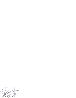
Figure 1: Phase diagram in the ${\bar{V}}$-${\bar{U}}$ plane showing the $\lambda$ dependence of the phase boundary between the gapless Luttinger liquid (LL) phase and the spin-gapped Luther-Emery liquid (LEL) phase, for an incommensurate 1DEG with $E_{F}/\omega_{0}=5$ (dashed lines) and $E_{F}/\omega_{0}=10$ (thin solid lines). The thick line shows the phase boundary at $\lambda=0$ for any $E_{F}/\omega_{0}$. $\lambda$ stands for either $\lambda_{\rm Hol}$ or $\lambda_{\rm Pei}$, depending on the model.

Figure 2: Phase diagram in the $\lambda l_{0}$-${\bar{U}}l_{0}$ plane for an incommensurate 1DEG, showing the dependence on ${\bar{V}}/{\bar{U}}$ of the phase boundary separating the LL and LEL phases. $\lambda$ stands for either $\lambda_{\rm Hol}$ or $\lambda_{\rm Pei}$, depending on the model.

We now study the effects of the el-ph interaction on the phase boundary between the LL and spin-gapped LEL. In Fig. 1 we show a phase diagram in the ${\bar{V}}$-${\bar{U}}$ plane, for various fixed values of $\lambda$ and $E_{F}/\omega_{0}$ (this phase boundary is the same for the Pei-Hub and Hol-Hub models). We see that a retarded el-ph interaction dramatically increases the stability of the LEL phase relative to the LL phase. The phase boundary is very sensitive to the retardation parameter $E_{F}/\omega_{0}$, with higher values favoring the LEL phase. For the case of an unretarded el-ph interaction ($\omega_{0}>E_{F}$), which is not typical in real materials, a spin gap can only occur for $\lambda>{\bar{U}}-2{\bar{V}}$. However, just a modest amount of retardation makes a spin gap possible, even, in some cases, for $\lambda\ll{\bar{U}}-2{\bar{V}}$. As we show in Section VI, this is due to the renormalization of the backscattering el-ph interaction toward stronger values. The figure shows that poorly screened interactions (high ${\bar{V}}/{\bar{U}}$) favor the LEL. The dependence of the phase boundary on ${\bar{V}}/{\bar{U}}$ is shown explicitly in Fig. 2, which presents a phase diagram in the $\lambda l_{0}$-${\bar{U}}l_{0}$ plane. This diagram shows that scaling eventually carries one to the case in which an infinitesimal $\lambda$ causes a spin gap (in other words, for $E_{F}\gg\omega_{0}$, the system is spin-gapped for infinitesimal $\lambda$).

III.1.2 Competition between spin density wave, charge density wave, and superconducting instabilities

Figure 3: Phase diagrams of the incommensurate extended Hol-Hub model with (a) $V=0$ and (b) ${\bar{V}}/{\bar{U}}=0.2$, and of the incommensurate extended Pei-Hub model for (c) $V=0$ and (d) ${\bar{V}}/{\bar{U}}=0.2$. For all diagrams, $E_{F}/\omega_{0}=10$. To the right of the thick line, the system is spin-gapped. The most divergent susceptibility is shown without parenthesis, while parenthesis indicate a susceptibility that diverges less strongly. SDW stands for $2k_{F}$ spin density wave, CDW stands for $2k_{F}$ charge density wave, SS stands for singlet superconductivity, and $4k_{F}$ stands for $4k_{F}$ charge density wave.

Figure 4: Phase diagrams of the incommensurate extended Hol-Hub model. (a) and (b) $\lambda_{\rm Hol}=0.2$; (c) and (d) $\lambda_{\rm Hol}=0.3$. (a) and (c) ${\bar{V}}/{\bar{U}}=0$; (b) and (d) ${\bar{V}}/{\bar{U}}=0.1$. Parenthesis indicate a subdominant susceptibility. The region with dominant SDW is the LL phase, while the rest of the parameter space is a LEL.

Below, we explore the many ordering instabilities present in the system. $2k_{F}$ spin density wave order (SDW), $2k_{F}$ charge density wave order (CDW), and singlet superconductivity (SS) can all compete at zero temperature. A divergent charge density wave susceptibility with $4k_{F}$ periodicity (labeled in phase diagrams as “$4k_{F}$”) is also possible. It is important to note that since long range order is forbidden in an incommensurate 1D system, the phase diagrams below actually consist of identifying instabilities with divergent response functions. However, for a quasi-1D array of weakly coupled chains, interchain coupling allows for true broken symmetry order at low temperature.

In Fig. 3 we present phase diagrams in the ${\bar{U}}$-$\lambda_{\rm Hol}$ and ${\bar{U}}$-$\lambda_{\rm Pei}$ planes, for $E_{F}/\omega_{0}=10$. In these diagrams, we show phase boundaries between regions where various ordering fluctuations have divergent susceptibilities in the low-temperature limit. The susceptibility that diverges most strongly, i.e., dominates, is shown without parenthesis. If a second susceptibility diverges, but less strongly, it is termed “subdominant,” and is shown in parenthesis. The thick solid line is the LL-LEL transition line; the LL phase is present to left of this line and the LEL phase to the right.

For repulsive el-el interactions, the entire LL phase, for either model, is dominated by SDW fluctuations, with a slightly weaker CDW susceptibility. The LEL phase is more complex. For the extended Hol-Hub model, dominant SS order is possible provided the el-el repulsion is weak enough and $\lambda_{\rm Hol}$ is neither too weak nor too strong. For the Pei-Hub model with repulsive el-el interactions, a phase with dominant SS is impossible due to the absence of el-ph forward scattering. Therefore, generally speaking, an optical phonon is more favorable to superconductivity than an acoustic one. In both models, there is a large region, for intermediate values of $\lambda$, with dominant CDW and subdominant SS. At high values of $\lambda$, SS is no longer divergent; in this region a $2k_{F}$ CDW dominates and a $4k_{F}$ CDW is subdominant. We must point out that the dashed line is not expected to be quantitatively accurate, since the method is a weak-coupling one. Note that the phase with dominant SS is strongly suppressed by poor screening (large ${\bar{V}}/{\bar{U}}$).

Figure 5: Phase diagram in the $g^{\prime}/\omega_{0}$-$t^{\prime}/\omega_{0}$ plane of the spinful incommensurate extended Hol-Hub model for (a) $U=V=0$; (b) $U^{\prime}/\omega_{0}=5$, $V=0$; and (c) $U^{\prime}/\omega_{0}=5$, ${\bar{V}}/{\bar{U}}=0.1$. Here $g^{\prime}\equiv g\sqrt{E_{F}/v_{F}}$, $t^{\prime}\equiv t(E_{F}/2t)$, and $U^{\prime}\equiv U(E_{F}/v_{F})$. In (a), a spin gap is present everywhere in the phase diagram, while in (b) and (c), it is present above the thick solid line.

In Fig. 4, we study the dependence of the ground state on $E_{F}/\omega_{0}$, for the Hol-Hub model, by showing phase diagrams in the $E_{F}/\omega_{0}$-${\bar{U}}$ plane. We see that high values of $E_{F}/\omega_{0}$ create a spin-gapped phase with dominant CDW. Low values of $E_{F}/\omega_{0}$ create a SS-dominated LEL for low ${\bar{U}}$, and a LL for high ${\bar{U}}$. In other words, an electron bandwidth that is too big is harmful to superconductivity! Note that for moderate $E_{F}/\omega_{0}$, the system lies in the region with dominant CDW and subdominant SS, which extends from ${\bar{U}}=0$ to quite large values of ${\bar{U}}$. Therefore, even when the bare interactions are predominantly repulsive (${\bar{U}}\gg\lambda_{\rm Hol}$), it is still possible for the system to have a divergent superconducting correlation. It is possible for this to occur even with a small degree of retardation like $E_{F}/\omega_{0}\sim 5$ [see Fig. 4(d)]. The phase diagram of the Pei-Hub model is similar to Fig. 4, except that the phase with dominant SS is removed, and the dashed line is shifted to slightly lower $E_{F}/\omega_{0}$.

It is worth pointing out the intriguing possibility that, for a quasi-1D system with dynamically fluctuating 1D chains, or even for chains that exhibit transverse spatial fluctuations, CDW order is easily dephased, while the superconducting instability is not.Nature If this is the case, then it is possible for the system to support superconductivity even for the physically realistic case of ${\bar{U}}\gg\lambda_{\rm Hol}$, and without the large amount of retardation that is required in 3D.

A number of authors have computed the phase diagram of the spinless Holstein model at half-filling, in the absence of el-el interactions (see Fig. 17). To facilitate comparison between this model and the spinful incommensurate extended Holstein-Hubbard model, Fig. 5 shows our phase diagram for the latter model, in units similar to Fig. 17.

III.1.3 Enhancement of superconductivity by repulsive interactions

The intuitive notion that repulsive interactions suppress superconductivity at weak-coupling, while always true in a Fermi liquid, does not always hold for the 1DEG coupled to phonons. In the 1DEG, the potentially strongly divergent part of the singlet superconducting susceptibility at temperature $T\ll\omega_{0}$ is $\chi_{\rm SS}\propto\Delta_{s}T^{1/K_{c}^{\rm eff}-2}$. Interactions in the spin channel determine $\Delta_{s}$, while charge interactions renormalize the effective Luttinger parameter $K_{c}^{\rm eff}$ away from its noninteracting value of 1 (see Section VI). Clearly, SS is enhanced by an increase in $\Delta_{s}$ or an increase in $K_{c}$. In many cases, increasing the el-el repulsion causes both $\Delta_{s}$ and $K_{c}$ to decrease. However, below we discuss cases in which one of the two parameters is increased by el-el repulsion; depending on how much the second parameter is reduced, $\chi_{\rm SS}$ may be enhanced.

In the absence of el-ph interactions, an increase in $U$ always decreases $K_{c}$ and $\Delta_{s}$, and therefore suppresses superconductivity. In a 1D el-ph system, this is often the case as well; however, there are also cases in which increasing $U$ can cause $K_{c}^{\rm eff}$ to be increased. (The technical reason is a decrease in the effective el-ph backscattering interaction–see Section VI.) Then, if $\Delta_{s}$ is not reduced too much by the increase in $U$, it is possible for SS to be enhanced. An example of this can be seen in Fig. 3(a) or 3(c). If we start at $\lambda=0.35$ and ${\bar{U}}=0$, and increase ${\bar{U}}$ while holding $\lambda$ fixed, we cross from a region without divergent SS to a region with divergent SS. This phenomenon can also be seen in Figs. 4(a) and 4(c) if the right value of $E_{F}/\omega_{0}$ is chosen [such as, for example, $E_{F}/\omega_{0}=200$ in Fig. 4(a)]. However, if we set ${\bar{V}}/{\bar{U}}\geq 1/6$ and hold this ratio fixed while increasing ${\bar{U}}$, superconductivity is never enhanced at weak coupling [see Figs. 3(b), 3(d), and Section VI].

In Fig. 6, we further investigate the enhancement of SS by repulsive interactions by plotting the dimensionless superconducting susceptibility

$$\bar{\chi}_{\rm SS}\equiv\pi v_{F}\chi_{\rm SS}=(\Delta_{s}/E_{F})(T/E_{F})^{1/K_{c}^{\rm eff}-2}$$ (6)

versus $\bar{U}$, at fixed $\lambda=0.3$, $V=0$, and $T/\omega_{0}=0.01$. For small ${\bar{U}}$, $\bar{\chi}_{\rm SS}$ increases with increasing ${\bar{U}}$. However, as ${\bar{U}}$ is increased further, $K_{c}^{\rm eff}$ stops increasing as rapidly, and the decreasing $\Delta_{s}$ causes $\bar{\chi}_{\rm SS}$ to drop back down.

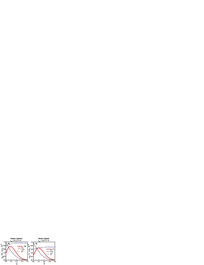
Figure 6: Dependence of the superconducting susceptibility $\bar{\chi}_{\rm SS}$ (thick line) on the Hubbard repulsion ${\bar{U}}$, for an incommensurate system with $V=0$, $E_{F}/\omega_{0}=10$, and $T/\omega_{0}=0.01$. (a) is for the Hol-Hub model with $\lambda_{\rm Hol}=0.3$, and (b) is for the Pei-Hub model with $\lambda_{\rm Pei}=0.3$. The thin line is $\Delta_{s}/\omega_{0}$ and the dashed line is the effective Luttinger exponent $K_{c}^{\rm eff}$.

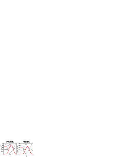
Figure 7: Dependence of $\bar{\chi}_{\rm SS}$ (thick line) on the nearest-neighbor repulsion ${\bar{V}}$, for an incommensurate system with ${\bar{U}=0.3}$, $E_{F}/\omega_{0}=10$, and $T/\omega_{0}=0.01$. (a) is for the Hol-Hub model with $\lambda_{\rm Hol}=0.2$, and (b) is for the Pei-Hub model with $\lambda_{\rm Pei}=0.2$. The thin line shows $\Delta_{s}/\omega_{0}$ and the dashed line is the effective Luttinger exponent $K_{c}^{\rm eff}$.

It is also possible to enhance superconductivity, in some cases, by increasing the nearest-neighbor Hubbard repulsion $V$, while holding $U$ fixed. This causes a renormalization of the el-ph backscattering toward stronger coupling, which results in an increase of $\Delta_{s}$ and a decrease of $K_{c}^{\rm eff}$. Depending on the competition between these two effects, $\chi_{\rm SS}$ may (or may not) be enhanced. An example of a case in which $\chi_{\rm SS}$ is enhanced can be seen in Figs. 3(a) and 3(c). There, if one begins at $\lambda=0.1$ and ${\bar{U}}=0.2$, then increases ${\bar{V}}/{\bar{U}}$ from 0 to 0.2 while holding $\lambda$ and ${\bar{U}}$ fixed, the system moves from a LL phase without divergent SS, to a LEL phase with divergent SS.

In Fig. 7, we explore this phenomenon further by plotting $\chi_{\rm SS}$ versus $\bar{V}$ at fixed ${\bar{U}}=0.3$, $\lambda=0.2$, and $T/\omega_{0}=0.01$. For small ${\bar{V}}$, $\chi_{\rm SS}$ is enhanced by increasing ${\bar{V}}$, due to the increase in $\Delta_{s}$. However, as ${\bar{V}}$ is increased further, eventually the rapidly decreasing $K_{c}^{\rm eff}$ begins to overwhelm the effect of the increasing $\Delta_{s}$, and $\chi_{\rm SS}$ decreases. In this case, optimizing superconductivity therefore requires a fine tuning of ${\bar{V}}/{\bar{U}}$.

We have pointed out exceptions to “rule” that el-el repulsion suppresses superconductivity at weak coupling, in order to illustrate, as a point of principle, the dramatically different physics that governs 1D el-ph systems compared with a Fermi liquid coupled to phonons. It is worth briefly discussing some prior works on this topic. Although the RG flow equations in Ref. Steve, are correct, the authors implied that an enhancement of superconductivity by repulsive interactions is a generic feature of the 1DEG coupled to phonons, while Ref. Voit2, concluded that repulsion always suppresses superconductivity. Our results indicate that both works overstated things; indeed, both situations are possible, depending on the choice of parameters. The disagreement between Ref. Steve, and Ref. Voit2, was caused, in large part, by the fact that Ref. Steve, focused purely on the effect of the el-ph interaction on $\Delta_{s}$, while Ref. Voit2, focused purely on the effect of the el-ph interaction on $K_{c}^{\rm eff}$. Above, we have correctly taken into account that the el-ph interaction affects both $\Delta_{s}$ and $K_{c}^{\rm eff}$, both of which in turn affect $\chi_{\rm SS}$.

III.2 Near half-filling

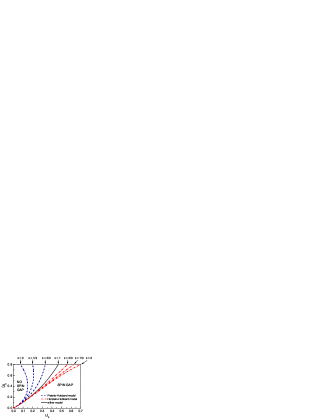
Figure 8: Dependence of the transition line between spin-gapped and non-spin-gapped phases on the doping parameter $\delta$ and on the electron-phonon model, for $V=0$. For $\mu\leq\omega_{0}$ (which includes the half-filled case $\mu=0$), the transition line is denoted by $\delta=0$. The incommensurate limit ($\mu\sim E_{F}$) is labeled by $\delta=1$. $\delta=1/3$ and 2/3 are intermediate dopings, with $\mu/\omega_{0}=(E_{F}/\omega_{0})^{\delta}$. Here, $\lambda$ stands for $\lambda_{\rm Pei}$ in the Pei-Hub model (dashed lines) and for $\lambda_{\rm Hol}$ in the Hol-Hub model (dashed-dotted lines). For $\delta=1$ (solid line), the transition line is the same for either model.

Figure 9: Doping dependence of the Hol-Hub phase diagram for $V=0$ and $E_{F}/\omega_{0}=5$. The value of $\delta$ is given above each plot.

Figure 10: Doping dependence of the Pei-Hub phase diagram for $V=0$ and $E_{F}/\omega_{0}=5$. The value of $\delta$ is given above each plot.

Figure 11: Phase diagrams for $E_{F}/\omega_{0}=5$ in the $\lambda$-$\delta$ plane. Plots (a) and (b) are for the Hol-Hub model; (c) and (d) are for the Pei-Hub model. Plots (a) and (c) are for ${\bar{U}}=0.1$; (b) and (d) are for ${\bar{U}}=0.4$. For all plots, $V=0$.

If we reduce the doping level of an incommensurate system (i.e., move closer to half-filling), the LL-LEL phase boundary is influenced in opposite ways for the Hol-Hub compared to the Pei-Hub model. This is because the on-site Hubbard repulsion is in direct competition with the attractive on-site el-ph interaction of the Holstein model, while it cooperates with the attractive bond centered interaction of the Pei model. Therefore, the spin gap is enhanced by proximity to half-filling for the Pei-Hub model, and reduced for the Hol-Hub model.

We illustrate this in Fig. 8, which presents a phase diagram in the ${\bar{U}}l_{0}$-$\lambda l_{0}$ plane, for $V=0$. This diagram shows the dependence of the LL-LEL phase boundary on the doping parameter

$$\delta=\frac{\ln(\mu/\omega_{0})}{\ln(E_{F}/\omega_{0})}.$$ (7)

Assuming the charge gap $\Delta_{c}<\mu$, the actual doping concentration $x$ relative to half-filling is related to $\delta$ by

$$x=\frac{2}{\pi v_{c}}\mu=\frac{2\omega_{0}}{\pi v_{c}}\left(\frac{E_{F}}{\omega_{0}}\right)^{\delta},$$ (8)

where $v_{c}\approx v_{F}$ is the charge velocity [see Eq. (41)]. The incommensurate limit $\delta=1$ is shown previously in Fig. 3(a) and Fig. 3(b) as a thick solid line. As we move closer to half-filling by lowering $\delta$, the LL-LEL transition line for the Pei-Hub model (dashed line) moves toward lower values of $\lambda$, while the transition line for the Hol-Hub model (dash-dotted line) moves toward higher values. In the weak-coupling limit assumed here, for $\mu\leq\omega_{0}$, the LL-LEL transition line is independent of $\mu$. Therefore, this phase boundary is the same for half-filling ($\mu=x=0$) as for $\delta=0$.

The doping dependencies of the other phase boundaries are shown in Figs. 9 and 10, for the range $\omega_{0}<\mu<E_{F}$. Figure 9 illustrates that for the Hol-Hub model, proximity to half-filling strongly suppresses the phase with dominant SS. For both models, moving toward half-filling increases the stability of the phase with subdominant $4k_{F}$ charge density wave, at the expense of the phase with subdominant SS, especially for the Pei-Hub model (Fig. 10). Note that, especially in Fig. 10, SS is divergent for a range of parameters such that $\bar{U}\gg\lambda_{\rm Pei}$, despite the low value of $E_{F}/\omega_{0}=5$. Figure 11 shows a different slice of the phase diagram by showing plots in the $\lambda$-$\delta$ plane.

III.3 Half-filling

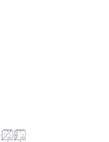
Figure 12: Phase diagram of the (a) half-filled Hol-Hub model and (b) half-filled Pei-Hub model, both with $V=0$. The dashed lines are for $E_{F}/\omega_{0}=5$ and the solid lines for $E_{F}/\omega_{0}=10$. For both diagrams, a spin gap is present for the CDW phase, while a charge gap is present everywhere in the phase diagram. In (b) the dotted line, defined by $\lambda_{\rm Pei}={\bar{U}}$, is the inaccurate result for the phase boundary from mean-field theory.

At half-filling, for repulsive el-el interactions, a charge gap is present for the entire phase diagram. Divergent SS is eliminated at half-filling. The region without a spin gap is a SDW, while the spin-gapped region is an ordered CDW. We show the half-filled phase diagram, for both models, in Fig. 12, for several values of $E_{F}/\omega_{0}$ and $V=0$. The difference between the two models is substantial, with the Pei-Hub model favoring CDW more than the Hol-Hub model. In Fig. 12(b), we also draw a dashed line defined by $\lambda_{\rm Pei}={\bar{U}}$, which is the transition line predicted by mean-field theory. Such a treatment is knownsalkola to be quite inaccurate for the Pei-Hub model, as demonstrated in the figure, since it does not take into account the dramatic renormalization of the backscattering el-ph interaction to stronger couplings. Note that the Pei-Hub phase diagram is very sensitive to $E_{F}/\omega_{0}$, with high values favoring a spin-gapped CDW, while the Hol-Hub phase diagram is only weakly dependent on $E_{F}/\omega_{0}$. It is interesting that in the Pei-Hub model [Fig. 12(b)], there is a maximum value of the critical el-ph coupling of about $0.149/l_{0}$, which occurs at ${\bar{U}}\approx 0.411/l_{0}$. (In other words, for $\lambda_{\rm Pei}>0.149/l_{0}$, the system is an ordered CDW for any ${\bar{U}}$.)

IV Doping dependence of the superconducting susceptibility and isotope effects

In this section, we study the strong doping dependencies of the spin gap, superconducting susceptibility, CDW susceptibility, and isotope effects.

Examining the phase diagram in Fig. 11(d), we can deduce an interesting nonmonotonic dependence of the SS susceptibility on $\delta$. For moderate values of $\lambda_{\rm Pei}$, for example, near $\lambda_{\rm Pei}\approx 0.2$, $\chi_{\rm SS}$ is not divergent near $\delta=0$, where only the $2k_{F}$ and $4k_{F}$ CDW susceptibilities diverge, nor is it divergent near $\delta=1$, where the system is in the gapless LL phase. However, $\chi_{\rm SS}$ is divergent for a certain range of moderate $\delta$. Therefore, in these cases, at fixed $T\ll\Delta_{s}$, $\chi_{\rm SS}$ must exhibit a maximum as a function of $\delta$ at some intermediate value of $\delta$.

This maximum in $\chi_{\rm SS}$, which occurs in both models, is shown explicitly in Figs. 13 and 14, where we plot ${\bar{\chi}}_{\rm SS}$ (thick solid line) versus $\delta$ at $T/\omega_{0}=0.1$, for representative parameters. The cause of the nonmonotonic doping dependence is the different doping dependencies of $\Delta_{s}$ and $K_{c}^{\rm eff}$. $\Delta_{s}$ decreases with increasing doping, which acts to reduce $\chi_{\rm SS}$, while $K_{c}^{\rm eff}$ increases with increasing doping, which acts to increase $\chi_{\rm SS}$. These two effects “compete” with each other and can cause a maximum at some “optimal” value of the doping that depends on the interaction strengths. The dimensionless $2k_{F}$ CDW susceptibility

$${\bar{\chi}}_{\rm CDW}\equiv\pi v_{F}\chi_{\rm CDW}=(\Delta_{s}/E_{F})(T/E_{F})^{K_{c}^{\rm eff}-2}$$ (9)

(dashed lines in Figs. 13 and 14) does not exhibit such a maximum, but instead decreases monotonically with increasing doping. In Figs. 13 and 14, we also plot $\Delta_{s}/\omega_{0}$ (thin solid lines), which shows that at low dopings, $\chi_{\rm SS}$ increases with increasing doping, despite the fact that the superconducting pairing strength $\Delta_{s}$ decreases.

We now consider the doping dependence of $T_{c}$ and the isotope effect on $T_{c}$ for a quasi-1D system that consists of an array of weakly coupled quasi-1D chains. We assume that the chains are spatially or dynamically fluctuating so that CDW order is dephased. The interchain Josephson coupling $J$ is treated on a mean-field level,arrigoni so that $T_{c}$ is determined by the temperature at which

$$2J\chi_{\rm SS}=1\;\;\;\;({\rm at}\;T=T_{c}),$$ (10)

where the numerical prefactor 2 is determined by the number of nearest-neighbor chains. Treating the interchain coupling with perturbative RG gives an equivalent result. Assuming $J$ is doping independent, $T_{c}$ then exhibits a maximum at the same $\delta$ where $\chi_{\rm SS}$ has a maximum.

The isotope effect exponent $\alpha_{T_{c}}$ is plotted versus $\delta$ in Fig. 15. It is shown for various values of ${\bar{J}}\equiv J/\pi v_{F}$, at fixed $\lambda$ and ${\bar{U}}$. Unlike in BCS theory, $\alpha_{T_{c}}$ is not universal but depends on the interaction strengths and band-filling. However, qualitatively, it appears that the doping-dependent behavior in which $\alpha_{T_{c}}$ is large near half-filling but decreases rapidly with increasing doping is generic (independent of interaction strengths and el-ph model). Note that if the parameters are tuned just right, $\alpha_{T_{c}}$ vanishes. A small $\alpha_{T_{c}}$ can even occur at the doping for which $T_{c}$ is maximum. Therefore, one should be careful not to assume that phonons are unimportant in unconventional superconductors for which $\alpha_{T_{c}}\ll 1$, such as in the cuprates at optimal doping. Figure 15 also shows $\alpha_{\Delta_{s}}$, which is weakly doping-dependent and negative.

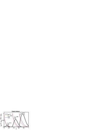
Figure 13: Doping dependence of the singlet superconducting susceptibility ${\bar{\chi}}_{\rm SS}$ (thick solid lines) at $T/\omega_{0}=0.1$, CDW susceptibility ${\bar{\chi}}_{\rm CDW}$ (dashed lines) at $T/\omega_{0}=0.1$, and spin gap (thin solid lines), for the Pei-Hub model with ${\bar{U}}=0.4$, $V=0$, $E_{F}/\omega_{0}=5$, and various values of $\lambda_{\rm Pei}$ (labeled in plot).

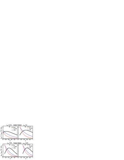
Figure 14: Doping dependence of ${\bar{\chi}}_{\rm SS}$ (thick solid lines) at $T/\omega_{0}=0.1$, ${\bar{\chi}}_{\rm CDW}$ (dashed lines) at $T/\omega_{0}=0.1$, and $\Delta_{s}/\omega_{0}$ (thin solid lines), for the Hol-Hub model [(a) and (b)], and the Pei-Hub model [(c) and (d)]. For all plots, ${\bar{U}}=0.1$, $V=0$, and $E_{F}/\omega_{0}=5$. The values of $\lambda_{\rm Hol}$ and $\lambda_{\rm Pei}$ are labeled above each plot.

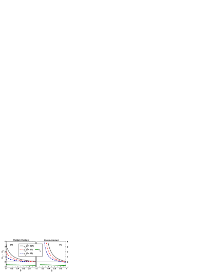
Figure 15: Dependence of the isotope effect exponents $\alpha_{T_{c}}$ and $\alpha_{\Delta_{s}}$ on the doping parameter $\delta$ and interchain coupling strength ${\bar{J}}$ for the Hol-Hub model with $\lambda_{\rm Hol}=0.275$ (a) and Pei-Hub model with $\lambda_{\rm Pei}=0.25$ (b). For both plots, ${\bar{U}}=0.1$, $V=0$, and $E_{F}/\omega_{0}=5$. $\alpha_{\Delta_{s}}$ is independent of ${\bar{J}}$.

V Comparison with other work

Below, we compare our results for the phase diagrams to some phase diagrams which have been previously computed.

V.1 Half-filled extended Peierls-Hubbard model

Figure 16: Phase diagram of the half-filled Pei-Hub model, comparing of our result for the phase boundary (solid line) to the quantum Monte Carlo result of Ref. Sengupta, (squares), for $U/t=2.5$ and $V/t=0.625$. The dashed line is our result for the same $U/t$ but with $V=0$. Here, $\tilde{\gamma}=\sqrt{\pi(\omega_{0}/t)\lambda_{\rm Pei}}/4$ is the el-ph coupling constant in Eq. (1).

We first compare our results for the half-filled extended Pei-Hub model to recent Monte Carlo work by Sengupta, Sandvik, and CampbellSengupta on the same model. Following Ref. Sengupta, , we show a phase diagram in the $\tilde{\gamma}$-$\omega_{0}/t$ plane in Fig. 16. This figure compares our result for the critical line for $U/t=2.5$ and $V/t=0.625$ (solid line) to the result in Ref. Sengupta, . (In order to plot our result in these units, we took the high-energy cutoff $E_{F}$ in the RG theory to be $t$.)

The quantitative disagreement near $\omega_{0}/t\sim 1$ can probably be attributed to the fact that the assumption in the RG theory of a linear electronic dispersion becomes problematic when $\omega_{0}\sim E_{F}$. At lower $\omega_{0}/t$, the agreement is excellent, especially considering the moderately strong value ${\bar{U}}=U/(2\pi t)\approx 0.4$. This gives one reason to believe that the multistep RG method is, at the very least, qualitatively accurate for physically interesting values of ${\bar{U}}\sim 1$.

In Fig. 16, we have also plotted our result for $V=0$ (dashed line), which can be obtained from the simple analytic expression in Eq. (58). The solid line in this figure is the only phase boundary in the present paper that required numerical integration of the RG flow equations [Eqs. (20) and (21)]. The phase boundaries in all other plots are given by analytic expressions derived in Section VI.

V.2 Holstein model

The phase diagram for perhaps the most interesting model studied in the present paper, the spinful incommensurate extended Holstein-Hubbard model, has not extensively studied in prior works. A much simpler related model, which has been thoroughly explored, is the spinless half-filled Holstein model (without el-el interactions). We show the phase diagram for this model in Fig. 17, computed by various authors with a wide range of methods. Note that the result from the two-step RG technique (line with squares)Caron is in good agreement with exact numerical methods.

In order to see how Fig. 17 changes when spin is included, we have computed a phase diagram in similar units for the spinful half-filled Holstein model in Fig. 18, including a Hubbard interaction. In the absence of el-el interactions, at weak el-ph coupling, the ground state of this model is always a CDW, for any finite $\omega_{0}$. This also holds in the strong coupling limit ($\lambda_{\rm Hol}\gg 1$).Fradkin2 In contrast, for the spinless half-filled Holstein model without el-el interactions, the transition to a CDW occurs at a nonzero value of $g$, as shown in Fig. 17 for weak coupling and proven in Ref. Fradkin2, for strong coupling.

To study how Fig. 18 changes when the system is doped into the incommensurate limit, we have presented a diagram in the same units for the spinful incommensurate extended Holstein-Hubbard model in Fig. 5. In Figs. 5 and 18, for technical reasons, we have defined $g^{\prime}=g\sqrt{E_{F}/v_{F}}$, $t^{\prime}=t(E_{F}/2t)$, and $U^{\prime}=U(E_{F}/v_{F})$.

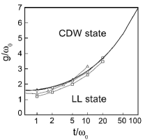
Figure 17: Phase diagram of the spinless half-filled Holstein model from various authors, in the absence of el-el interactions. The solid line is an analytical result from Ref. Wang, . The line with circles and the line with squares denote the results of density matrix renormalization group (Ref. Bursill, ) and two-step RG (Ref. Caron, ), respectively. The line with triangles is the result from an exact-diagonalization method (Ref. Weisse, ). (After Ref. Wang, .)

Figure 18: Phase diagram in the $g^{\prime}/\omega_{0}$-$t^{\prime}/\omega_{0}$ plane of the spinful half-filled Holstein-Hubbard model for $V=0$. The phase boundary is shown for various values of $U^{\prime}/\omega_{0}$, as labeled. The system is charge-gapped everywhere in the phase diagram, and spin-gapped in the CDW phase. For $U^{\prime}/\omega_{0}=0$ (not shown), the ground state is a CDW for infinitesimal $g^{\prime}/\omega_{0}$. Here, $g^{\prime}\approx g$, $t^{\prime}\approx t$, and $U^{\prime}\approx U$ (see the text for their precise definitions).

VI Methods and derivations

Here, we provide more discussion of the technique and study the RG flows of the coupling parameters. We also derive the explicit expressions that were used to plot the phase boundaries in the figures.

VI.1 Field theory for the 1DEG coupled to phonons

To focus on the low-energy, long-wavelength physics, we work with continuum versions of Eqs. (1) and (4). The purely electronic part of our Hamiltonian is the standard continuum model of the interacting 1DEG, in which the spectrum is linearized around the left and right Fermi points. The destruction field for fermions of spin $\sigma$ is written as a sum of slowly varying right and left moving fields: $\Psi_{\sigma}=e^{ik_{F}x}\psi_{1,\sigma}+e^{-ik_{F}x}\psi_{-1,\sigma}$. The Hamiltonian density for the 1DEG, in the absence of el-ph interactions, is written as ${\cal H}={\cal H}_{0}+{\cal H}_{\rm el-el}$, where the kinetic energy density is

$${\cal H}_{0}=-iv_{F}\sum_{\eta,\sigma=\pm 1}\eta\,\psi_{\eta,\sigma}^{\dagger}\partial_{x}\psi_{\eta,\sigma},$$ (11)

and the important short range el-el interaction terms are

$${\cal H}_{\rm el-el} = g_{1}\sum_{\sigma,\sigma^{\prime}=\pm 1}\psi_{1,\sigma}^{\dagger}\psi_{-1,\sigma^{\prime}}^{\dagger}\psi_{1,\sigma^{\prime}}\psi_{-1,\sigma}$$ (12)

$$+ g_{2}\sum_{\sigma,\sigma^{\prime}=\pm 1}\psi_{1,\sigma}^{\dagger}\psi_{-1,\sigma^{\prime}}^{\dagger}\psi_{-1,\sigma^{\prime}}\psi_{1,\sigma}$$

$$+ g_{3}\,[e^{i(4k_{F}-G)x}\,\psi_{-1,1}^{\dagger}\psi_{-1,-1}^{\dagger}\psi_{1,-1}\psi_{1,1}+{\rm H.c.}]$$

$$+ g_{4}\sum_{\eta,\sigma=\pm 1}\psi_{\eta,\sigma}^{\dagger}\psi_{\eta,-\sigma}^{\dagger}\psi_{\eta,-\sigma}\psi_{\eta,\sigma}.$$

We have assumed the system is spin-rotation invariant. The $g_{2}$ and $g_{4}$ terms describe forward scattering, the former containing scattering on both left and right moving branches, and the latter containing scattering on only one branch. The $g_{1}$ term contains backscattering from one branch to the other. The $g_{3}$ term contains Umklapp processes and is only important when $4k_{F}$ equals a reciprocal lattice vector $G$; i.e., at half-filling ($4k_{F}=2\pi$). For the extended Hubbard model in the continuum limit, the bare (unrenormalized) values of the $g_{i}$’s are given by

$$g_{1}^{0} = g_{3}^{0}\>=\>U-2V^{\prime},$$ (13)

$$g_{2}^{0} = U+2V^{\prime},$$ (14)

$$g_{4}^{0} = U/2+2V^{\prime}$$ (15)

where the superscript $0$ indicates bare couplings and again $V^{\prime}=-V\cos(2k_{F})$, which equals $V$ at half-filling.

We incorporate el-ph interactions by defining retarded interactions $g_{1,{\rm ph}}$, $g_{2,{\rm ph}}$, $g_{3,{\rm ph}}$, and $g_{4,{\rm ph}}$ which play the same role as the $g_{i}$’s except that the energy transfer is restricted to be less than a cutoff $\omega_{c}$, which is approximately the phonon frequency $\omega_{0}$ ($\omega_{c}$ will be defined more precisely below). This corresponds to approximating the phonon propagator as a step function of frequency, which is a good approximation for the momentum-independent phonon dispersions we consider in this paper. In the Pei-Hub model, the bare el-ph couplings are given by

$$g_{1,{\rm ph}}^{0} = -g_{3,{\rm ph}}^{0}\>=\>-\pi v_{F}\lambda_{\rm Pei},$$ (16)

$$g_{2,{\rm ph}}^{0} = g_{4,{\rm ph}}^{0}\>=\>0.$$ (17)

For the Hol-Hub model they are

$$g_{1,{\rm ph}}^{0}=g_{2,{\rm ph}}^{0}=g_{3,{\rm ph}}^{0}=g_{4,{\rm ph}}^{0}=-\pi v_{F}\lambda_{\rm Hol},$$ (18)

where $\lambda_{\rm Pei}$ and $\lambda_{\rm Hol}$ are the positive, dimensionless coupling constants defined in Eq. (II). Note that the couplings $g_{1,{\rm ph}}^{0}$, $g_{2,{\rm ph}}^{0}$, and $g_{4,{\rm ph}}^{0}$ are negative, indicating the attractive interaction induced by phonons. In the absence of el-el interactions, the sign of $g_{3,{\rm ph}}^{0}$ is arbitrary; likewise, the sign of $g_{3}^{0}$ is arbitrary in the absence of el-ph interactions. However, for the extended Hubbard model coupled to phonons, once the sign convention $g_{3}^{0}=U-2V^{\prime}$ is chosen, it is required that $g_{3,{\rm ph}}^{0}>0$ for the Pei-Hub model and $g_{3,{\rm ph}}^{0}<0$ for the Hol-Hub model.

VI.2 Phase diagram of the 1DEG without phonons

Before deriving the phase diagram including phonons, we briefly review the known quantum phase diagram of the 1DEG without el-ph coupling,giamarchi ; giamarchiPaper ; KivelsonBook by identifying the conditions for various types of order to have divergent susceptibilities in the low-temperature limit.

The sign of $g_{1}^{0}$ determines the existence or nonexistence of a spin gap: a 1DEG without el-ph coupling contains a gap to spin excitations for $g_{1}^{0}<0$, and no such gap for $g_{1}^{0}\geq 0$, regardless of band filling. A charge gap is only possible at commensurate fillings.

Table 1: Conditions for various ordering fluctuations to dominate for an incommensurate 1DEG. See the text for the subdominant fluctuations.

Type of order	Dominates for
$4k_{F}$ charge density wave ($4k_{F}$)	$\Delta_{s}=0$, $K_{c}<1/3$
$2k_{F}$ spin density wave	$\Delta_{s}=0$, $1/3<K_{c}<1$
$2k_{F}$ charge density wave	$\Delta_{s}>0$, $K_{c}<1$
Triplet superconductivity	$\Delta_{s}=0$, $K_{c}>1$
Singlet superconductivity	$\Delta_{s}>0$, $K_{c}>1$

Table 2: Conditions for SDW and CDW order in a half-filled, charge-gapped 1DEG.

Type of order	Present for
$2k_{F}$ spin density Wave	$\Delta_{s}=0$
$2k_{F}$ charge Density Wave	$\Delta_{s}>0$

An incommensurate 1DEG without a spin gap (Luttinger liquid), has a divergent $2k_{F}$ SDW susceptibility when the Luttinger charge exponent

$$K_{c}=\sqrt{\frac{2\pi v_{F}+2g_{4}^{0}+g_{1}^{0}-2g_{2}^{0}}{2\pi v_{F}+2g_{4}^{0}-g_{1}^{0}+2g_{2}^{0}}}$$ (19)

is less than 1, along with a logarithmically more weakly divergent $2k_{F}$ CDW correlation. If $K_{c}<1/2$, the $4k_{F}$ CDW correlation is also divergent; it is less divergent than SDW and $2k_{F}$ CDW for $1/3<K_{c}<1/2$, but becomes the dominant order for $K_{c}<1/3$. For $K_{c}>1$, a LL has a divergent triplet superconducting (TS) correlation and a logarithmically weaker divergent singlet superconductivity.

An incommensurate spin-gapped 1DEG (Luther-Emery liquid), is dominated by either SS or $2k_{F}$ CDW correlations, depending on the value of $K_{c}$. A LEL with $K_{c}<1$ is dominated by $2k_{F}$ CDW. If $K_{c}<1/2$, $4k_{F}$ CDW is subdominant, while if $1/2<K_{c}<1$, SS fluctuations replace $4k_{F}$ CDW as the subdominant order. For $1<K_{c}<2$, SS is the most divergent channel, and CDW is subdominant. For $K_{c}>2$, the only divergent correlations is SS. We summarize the phase diagram of the incommensurate 1DEG in Table 1.

At half-filling, a 1DEG is charge-gapped for $|g_{3}^{0}|>g_{1}^{0}-2g_{2}^{0}$, which for repulsive interactions is always satisfied. For $g_{1}^{0}<0$, the ground state of a charge-gapped system is an ordered, spin-gapped CDW (the Peierls instability), otherwise, it is a SDW with no spin gap.

VI.3 The multistep RG technique

To determine the phase diagrams, we apply the known one-loop RG flow equationsSteve

$$\frac{dg_{1}}{dl}=-g_{1}^{2},\;\;\>\frac{dg_{c}}{dl}=-g_{3}^{2},\;\;\>\frac{dg_{3}}{dl}=-g_{3}g_{c},\;\;\;\;\;$$ (20)

$$\frac{dg_{\pm,{\rm ph}}}{dl}=-g_{\pm,{\rm ph}}\left(\frac{3}{2}g_{1}\pm g_{3}+\frac{1}{2}g_{c}+g_{\pm,{\rm ph}}\right),$$ (21)

$$\frac{dg_{2,{\rm ph}}}{dl}=\frac{dg_{4,{\rm ph}}}{dl}=\frac{dg_{4}}{dl}=0,$$ (22)

$$\frac{d\omega_{c}}{dl}=\omega_{c}(\pi v_{F}+g_{+,{\rm ph}}),\;\;\>\frac{d\mu}{dl}=\pi v_{F}\mu,$$ (23)

where we defined

$$\;g_{c}=g_{1}-2g_{2},$$ (24)

$$\;g_{\pm,{\rm ph}}=g_{1,{\rm ph}}\pm g_{3,{\rm ph}},$$ (25)

$$\;l=(\pi v_{F})^{-1}\ln(E_{F}/\omega),$$ (26)

and $\omega$ is the running cutoff. The above expressions apply for $E_{F}\gg\omega\gg\omega_{0},\mu$. If, instead, $\mu\gg\omega\gg\omega_{0}$, the same equations apply, but with $g_{3}=g_{3,{\rm ph}}=0$. ¿From Eq. (20), we see that a repulsive $g_{1}$ renormalizes in the same way as the Coulomb pseudopotential in a Fermi liquid–it is scaled to smaller values as one integrates out high-energy degrees of freedom. However, in 1D the backscattering and Umklapp el-ph interactions $g_{1,{\rm ph}}$ and $g_{3,{\rm ph}}$ are strongly renormalized. Furthermore, there are cross terms $g_{\pm,{\rm ph}}g_{i}$ in Eq. (21), which means that the RG flows of $g_{1,{\rm ph}}$ and $g_{3,{\rm ph}}$ are strongly influenced by direct el-el interactions.

The two-step RG procedure is as follows: Assuming $\Delta_{s}<\omega_{0}$ and the system is at half-filling ($\mu=0$), we first integrate out fermionic degrees of freedom between the high-energy scale $E_{F}$ and the phonon energy $\omega_{0}$ using Eqs. (20) and (21). Once $\omega_{0}$ is reached, total effective interactions $g_{i}^{\rm tot}(\omega_{0})$ at this energy scale are determined by adding the effective el-el coupling to the effective el-ph coupling

$$g_{i}^{\rm tot}(\omega_{0})=g_{i}(\omega_{0})+g_{i,{\rm ph}}(\omega_{0}).$$ (27)

Below this energy scale, there is no difference between retarded and instantaneous interactions, so $g_{i}^{\rm tot}$ renormalizes as a non-retarded interaction using Eq. (20) with $g_{i}^{\rm tot}(\omega_{0})$ as the initial value. If the system is far enough away from half-filling such that $\mu\sim E_{F}$, the method is identical except that one sets $g_{3}^{0}=g_{3,{\rm ph}}^{0}=0$ at the start. For the above cases, it is clear that the renormalized couplings $g_{i}^{\rm tot}(\omega_{0})$ and the renormalized cutoff $\omega_{0}$ play the same role in the 1D electron-phonon system as $g_{i}^{0}$ and $E_{F}$, respectively, do in the pure 1DEG. Therefore, to determine the phase diagram of the 1DEG coupled to phonons, we can use the known phase diagram of the pure 1DEG, and simply replace the $g_{i}^{0}$’s there with $g_{i}^{\rm tot}(\omega_{0})$’s. For more general fillings ($0<\mu<E_{F}$), a three-step RG method is necessary, which we will elaborate at the end of this section.

Note that $\omega_{0}$ is the physical phonon frequency, which is related to $\omega_{c}$ by the expression $\omega_{0}=\omega_{c}(\omega_{0})$, where $\omega_{c}(\omega_{0})$ is the renormalized value of $\omega_{c}$ at the energy scale $\omega_{0}$, determined by Eq. (23). Likewise, we define $\mu$ as the physical value of the chemical potential relative to its value at half-filling; the bare chemical potential $\mu^{0}$ is chosen such that it flows to the value $\mu$ after integrating out degrees of freedom between $E_{F}$ and $\mu$.

VI.4 Incommensurate filling

We first derive the scaling of the coupling constants and compute the phase diagrams for the case when the system is doped far into the incommensurate limit ($\mu\sim E_{F}$).

VI.4.1 Scaling of the coupling constants

Using Eqs. (20) and (21) with $g_{3}=g_{3,{\rm ph}}=0$, we integrate out degrees of freedom between $E_{F}$ and $\omega$ with $E_{F}>\omega\geq\omega_{0}$, to obtain the follow effective couplings for incommensurate systems:

$$g_{c}(\omega) = g_{c}^{0},$$ (28)

$$g_{1}(\omega) = \frac{g_{1}^{0}}{1+g_{1}^{0}l},$$ (29)

$$g_{1,{\rm ph}}(\omega) = \left(\frac{g_{1,{\rm ph}}^{0}}{1+g_{1,{\rm ph}}^{0}Z}\right)\left(\frac{g_{1}(\omega)}{g_{1}^{0}}\right)^{3/2}\left(\frac{E_{F}}{\omega}\right)^{-g_{c}^{0}/2\pi v_{F}},$$

where

$$Z=\int_{0}^{l}dx\,\frac{\exp(-g_{c}^{0}x/2)}{(1+g_{1}^{0}x)^{3/2}},$$ (31)

and again $g_{i}^{0}=g_{i}(E_{F})$.

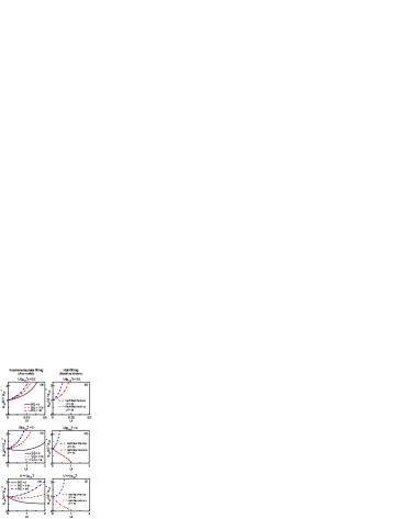
Figure 19: Dependence of the effective backscattering el-ph coupling $g_{1,{\rm ph}}(\omega)$ on $Ul\equiv(U/\pi v_{F})\ln(E_{F}/\omega)$ for $\omega>\omega_{0}$. Plots (a), (c), and (e) are for systems doped into the incommensurate limit, while (b), (d) and (f) are for the half-filled Pei-Hub and Hol-Hub models with $V=0$. For each plot, the ratio of $U$ to the bare el-ph coupling $g_{1,{\rm ph}}^{0}$ is held fixed at the value indicated above the plot. For each curve in (a), (c), and (e), the ratio ${\bar{V}}/{\bar{U}}$ is held fixed at the value indicated.

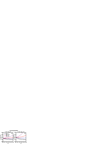
Figure 20: Dependence of $g_{1,{\rm ph}}(\omega_{0})$ on ${\bar{U}}$ for incommensurate systems with (a) $E_{F}/\omega_{0}=5$ and (b) $E_{F}/\omega_{0}=10$ (b). The horizontal dotted line indicates the value of the bare el-ph coupling $\lambda=-g_{1,{\rm ph}}^{0}/\pi v_{F}=0.2$, where $\lambda$ stands for either $\lambda_{\rm Hol}$ or $\lambda_{\rm Pei}$, depending on the model. For each curve, the ratio ${\bar{V}}/{\bar{U}}$ is held fixed at the value indicated in (a).

In the absence of el-el interactions, the el-ph backscattering coupling $g_{1,{\rm ph}}$ flows to stronger values according to $g_{1,{\rm ph}}(\omega)/g_{1,{\rm ph}}^{0}=(1-|g_{1,{\rm ph}}^{0}|l)^{-1}$. In Fig. 19, the important influence of extended Hubbard interactions on $g_{1,{\rm ph}}(\omega)$ in studied. In Figs. 19(a) and 19(c), we show the scaling for several fixed finite values of $U/|g_{1,{\rm ph}}^{0}|$. Fig. 19(e) shows the scaling in the limit $U\gg|g_{1,{\rm ph}}^{0}|$, which is given by

$$g_{1,{\rm ph}}(\omega)/g_{1,{\rm ph}}^{0}\approx h(Ul),\;\;\;\;\;\;(U\gg|g_{1,{\rm ph}}^{0}|),$$ (32)

where for future convenience we define

$$h(x) = \frac{\exp(G_{c}x/2)}{(1+G_{1}x)^{3/2}},$$ (33)

$$G_{1} = 1-2({\bar{V}}/{\bar{U}}),$$ (34)

$$G_{c} = 1+6({\bar{V}}/{\bar{U}}).$$ (35)

¿From Fig. 19, we see that the flow of $g_{1,{\rm ph}}$ is very sensitive to the parameter ${\bar{V}}/{\bar{U}}$. If ${\bar{V}}/{\bar{U}}<1/6$ and $U/|g_{1,{\rm ph}}^{0}|$ is large enough, then the $g_{\pm,{\rm ph}}g_{1}$ term in Eq. (21) causes $g_{1,{\rm ph}}(\omega)$ to initially flow to weaker values. However, if ${\bar{V}}/{\bar{U}}\geq 1/6$, then $g_{1,{\rm ph}}(\omega)/g_{1,{\rm ph}}^{0}>1$ for all $\omega<E_{F}$, regardless of $U/|g_{1,{\rm ph}}^{0}|$. The driving force for this increase in $|g_{1,{\rm ph}}(\omega)|$ is the $g_{\pm,{\rm ph}}g_{c}$ term in Eq. (21).

To better understand why increasing ${\bar{U}}$ can sometimes enhance superconductivity at small ${\bar{U}}$ (see Fig. 6), we study the dependence of $g_{1,{\rm ph}}(\omega_{0})$ on ${\bar{U}}$ at fixed $E_{F}/\omega_{0}$ in Fig. 20. In this plot, for small ${\bar{U}}$, the effective $g_{1,{\rm ph}}$ is stronger that its bare value ($g_{1,{\rm ph}}(\omega_{0})/g_{1,{\rm ph}}^{0}>1$). However, for ${\bar{V}}/{\bar{U}}<1/6$, increasing ${\bar{U}}$ causes $|g_{1,{\rm ph}}(\omega_{0})|$ to decrease. This can cause $K_{c}^{\rm eff}$ and $\chi_{\rm SS}$ to increase, as in Fig. 6. However, if we set ${\bar{V}}/{\bar{U}}\geq 1/6$ and hold this ratio fixed while increasing ${\bar{U}}$, then $|g_{1,{\rm ph}}(\omega_{0})|$ increases, causing $K_{c}^{\rm eff}$ and $\chi_{\rm SS}$ to be suppressed.

Note that in real materials, one typically expects ${\bar{V}}/{\bar{U}}>1/6$, in which case $|g_{1,{\rm ph}}(\omega_{0})|>|g_{1,{\rm ph}}^{0}|$ or even $|g_{1,{\rm ph}}(\omega_{0})|\gg|g_{1,{\rm ph}}^{0}|$. The requirement for a spin gap is $|g_{1,{\rm ph}}(\omega_{0})|>g_{1}(\omega_{0})$, which can be achieved, in many cases, with even a small amount of retardation. (Note that for repulsive el-el interactions, $0<g_{1}(\omega_{0})<g_{1}^{0}$.) Therefore, it is possible for a slightly retarded el-ph interaction to create a divergent superconducting susceptibility even when the bare interactions are predominantly repulsive ($|g_{1,{\rm ph}}^{0}|\ll g_{1}^{0}$).

VI.4.2 Luttinger liquid to Luther-Emery liquid transition

The phase boundary between the LL and LEL phases is given by the condition $g_{1}^{\rm tot}(\omega_{0})=0$. This condition determines the following critical value of the bare el-ph coupling

$$\lambda^{\rm Gap}_{\rm Pei}=\lambda^{\rm Gap}_{\rm Hol} = {\bar{U}}\left[\frac{\exp(G_{c}{\bar{U}}l_{0}/2)}{G_{1}\sqrt{1+G_{1}{\bar{U}}l_{0}}}+f({\bar{U}}l_{0})\right]^{-1}\;\;\;\;$$

$${\rm(LL{\rm-}LEL\;transition)},$$

where we define

$$f(y)=\int_{0}^{y}dx\,h(x).$$ (37)

For $\lambda_{\rm Pei}>\lambda^{\rm Gap}_{\rm Pei}$ or $\lambda_{\rm Hol}>\lambda^{\rm Gap}_{\rm Hol}$, the ground state of the incommensurate 1DEG is a spin-gapped LEL; otherwise, it is a gapless LL. The condition $\lambda=\lambda^{\rm Gap}_{\rm Pei}=\lambda^{\rm Gap}_{\rm Hol}$ therefore determines the transition lines in Figs. 1 and 2, as well as the thick solid lines in Figs. 3, 4, and 5. Note that in Fig. 2, we used that the “scaled” critical couplings $\lambda^{\rm Gap}_{\rm Hol}l_{0}$ and $\lambda^{\rm Gap}_{\rm Pei}l_{0}$ depend only on the two parameters ${\bar{U}}l_{0}$ and ${\bar{V}}/{\bar{U}}$.

VI.4.3 Susceptibilities and spin gap in the LEL phase

In the LEL phase, the potentially strongly divergent part of the low-temperature susceptibilities for SS and $2k_{F}$ CDW are given by Eqs. (6) and (9), respectively, where $K_{c}^{\rm eff}$ is the effective Luttinger charge exponent after integrating out states between $E_{F}$ and $\omega_{0}$, given by

$$K_{c}^{\rm eff}=\sqrt{\frac{2\pi v_{F}+2g_{4}^{\rm tot}+g_{c}^{\rm tot}(\omega_{0})}{2\pi v_{F}+2g_{4}^{\rm tot}-g_{c}^{\rm tot}(\omega_{0})}},$$ (38)

where

$$g_{c}^{\rm tot}(\omega_{0}) = g_{c}^{0}+g_{1,{\rm ph}}(\omega_{0})-2g_{2,{\rm ph}}^{0},$$ (39)

$$g_{4}^{\rm tot} = g_{4}^{0}+g_{4,{\rm ph}}^{0}.$$ (40)

Integrating out states below the energy $\omega_{0}$ does not further renormalize $g_{c}^{\rm tot}$ (and therefore $K_{c}$). Note that the effective charge and spin velocities are also renormalized due to phonons, the former of which is

$$v_{c}=(2\pi)^{-1}\sqrt{[2\pi v_{F}+2g_{4}^{\rm tot}]^{2}-[g_{c}^{\rm tot}(\omega_{0})]^{2}}.$$ (41)

For $-1<g_{1}^{\rm tot}(\omega_{0})<0$, $\Delta_{s}$ is given approximately by the energy scale below $\omega_{0}$ at which the RG analysis breaks down because the effective $g_{1}^{\rm tot}/\pi v_{F}$ has grown to $-1$. Since

$$g_{1}^{\rm tot}(\omega)=\frac{g_{1}^{\rm tot}(\omega_{0})}{1+[g_{1}^{\rm tot}(\omega_{0})/\pi v_{F}]\ln(\omega_{0}/\omega)}\;\;\;\;\;{\rm for}\;\omega<\omega_{0},$$

this gives

$$\Delta_{s}=\omega_{0}e\exp[-\pi v_{F}/|g_{1}^{\rm tot}(\omega_{0})|].$$ (42)

For $g_{1}^{\rm tot}(\omega_{0})>0$, $g_{1}^{\rm tot}(\omega)\rightarrow 0$ as $\omega\rightarrow 0$; therefore, $\Delta_{s}=0$.

VI.4.4 Competition between SS and CDW in the Hol-Hub model

The thin solid line in the incommensurate extended Hol-Hub model phase diagrams of Figs. 3, 4, and 5, which we call the “superconducting transition,” is determined by $K_{c}^{\rm eff}=1$. This condition is satisfied for $\lambda_{\rm Hol}=\lambda^{{\rm SS},+}_{\rm Hol}$ and $\lambda_{\rm Hol}=\lambda^{{\rm SS},-}_{\rm Hol}$ where

$$\lambda^{{\rm SS},\pm}_{\rm Hol}={\bar{U}}\left[H\pm\sqrt{H^{2}-\frac{G_{c}}{2f({\bar{U}}l_{0})}}\right]\;\;\;\;$$ (43)

$$\;\;\;\;\;\;{\rm(superconducting\;transition)}$$

and

$$H=\frac{2-h({\bar{U}}l_{0})}{4f({\bar{U}}l_{0})}+\frac{G_{c}}{4}.$$ (44)

Therefore, as long as the square root is not imaginary, for fixed ${\bar{U}}l_{0}>0$, there are two critical values of the bare el-ph coupling determining the boundary between the phase with dominant CDW and the phase with dominant SS. The most divergent correlation is SS provided $G_{c}<2f({\bar{U}}l_{0})H^{2}$ and $\lambda^{{\rm SS},-}_{\rm Hol}<\lambda_{\rm Hol}<\lambda^{{\rm SS},+}_{\rm Hol}$. Note that divergent a TS susceptibility is not present in any phase diagrams, since for repulsive el-el interactions, $K_{c}^{\rm eff}<1$ whenever $g_{1}^{\rm tot}(\omega_{0})>0$.

The phase boundary shown as a dashed line in Figs. 3, 4, and 5 is defined by $K_{c}^{\rm eff}=1/2$. For the extended Hol-Hub model, this condition occurs at $\lambda_{\rm Hol}=\lambda^{\rm CDW}_{\rm Hol}$ with

$$\lambda^{\rm CDW}_{\rm Hol}={\bar{U}}\left[L+\sqrt{L^{2}+\frac{Q}{2f({\bar{U}}l_{0})}}\right]\;\;\;\;$$ (45)

$$\;\;\;\;{\rm(}K_{c}^{\rm eff}=1/2\;{\rm transition),}$$

where

$$L = \frac{4-5h({\bar{U}}l_{0})}{8f({\bar{U}}l_{0})}-\frac{Q}{4},$$ (46)

$$Q = 3/{\bar{U}}-9({\bar{V}}/{\bar{U}})-1.$$ (47)

For $\lambda_{\rm Hol}>\lambda^{\rm CDW}_{\rm Hol}$, a divergent SS susceptibility is not possible.

VI.4.5 Competition between SS and CDW in the Pei-Hub model

For the extended Pei-Hub model with repulsive el-el couplings, $K_{c}^{\rm eff}<1$ always, which means a phase with dominant SS is impossible. For this model the condition $K_{c}^{\rm eff}=1/2$ occurs at the critical el-ph coupling value

$$\lambda^{\rm CDW}_{\rm Pei}={\bar{U}}\left[\frac{5h({\bar{U}}l_{0})}{2Q}+f({\bar{U}}l_{0})\right]^{-1}\;\;$$ (48)

$$\;\;\;\;{\rm(}K_{c}^{\rm eff}=1/2\;{\rm transition)}.$$

For $\lambda_{\rm Pei}>\lambda^{\rm CDW}_{\rm Pei}$, the SS susceptibility is never divergent. The condition $\lambda_{\rm Pei}=\lambda^{\rm CDW}_{\rm Pei}$ determines the dashed line in Figs. 3(c) and 3(d).

VI.5 Half-filling

At half-filling, Eqs. (20) and (21) can be integrated analytically if one takes $g_{c}^{0}=-g_{3}^{0}$. For that case,

$$g_{c}(\omega) = -g_{3}(\omega)=\frac{g_{c}^{0}}{1+g_{c}^{0}l},$$ (49)

$$g_{+,{\rm ph}}(\omega) = \left(\frac{g_{+,{\rm ph}}^{0}}{1+g_{+,{\rm ph}}^{0}X}\right)\left(\frac{g_{1}(\omega)}{g_{1}^{0}}\right)^{3/2}\left(\frac{g_{c}(\omega)}{g_{c}^{0}}\right)^{-1/2},$$

$$g_{-,{\rm ph}}(\omega) = \left(\frac{g_{-,{\rm ph}}^{0}}{1+g_{-,{\rm ph}}^{0}Y}\right)\left(\frac{g_{1}(\omega)}{g_{1}^{0}}\right)^{3/2}\left(\frac{g_{c}(\omega)}{g_{c}^{0}}\right)^{3/2},$$

where

$$X=\int_{0}^{l}dx\,(1+g_{1}^{0}x)^{-3/2}(1+g_{c}^{0}x)^{1/2},\;\;\;\;\;\;\;\;\;\;\;\;\;\;\;\;\;\;\;\;$$ (52)

$$Y=\int_{0}^{l}dx\,(1+g_{1}^{0}x)^{-3/2}(1+g_{c}^{0}x)^{-3/2}\;\;\;\;\;\;\;\;\;\;\;\;\;\;\;\;\;\;\;\;$$

$$\;\;=\frac{2}{(g_{1}^{0}-g_{c}^{0})^{2}}\left[g_{1}^{0}+g_{c}^{0}-\frac{g_{1}^{0}+g_{c}^{0}+2g_{1}^{0}g_{c}^{0}l}{\sqrt{(1+g_{1}^{0}l)(1+g_{c}^{0}l)}}\right],\,\;\;$$ (53)

and $g_{1}(\omega)$ is given again by Eq. (29). Since our assumption of $g_{c}^{0}=-g_{3}^{0}$ is satisfied for the Hubbard model (with $V=0$), the above results determine the scalings of $g_{1,{\rm ph}}$ and $g_{3,{\rm ph}}$ for the Hol-Hub and Pei-Hub models, which are

$$g_{1,{\rm ph}}(\omega)=g_{3,{\rm ph}}(\omega)=\left(\frac{g_{1,{\rm ph}}^{0}}{1+g_{1,{\rm ph}}^{0}X^{\prime}}\right)\sqrt{\frac{1-Ul}{(1+Ul)^{3}}}$$

$$\;\;\;\;\;\;({\rm half{\rm-}filled\;Holstein{\rm-}Hubbard\;model}),$$ (54)

$$g_{1,{\rm ph}}(\omega)=-g_{3,{\rm ph}}(\omega)=\left(\frac{g_{1,{\rm ph}}^{0}}{1+g_{1,{\rm ph}}^{0}Y^{\prime}}\right)\sqrt{\frac{1}{[1-(Ul)^{2}]^{3}}}$$

$$\;\;\;\;\;\;\;\;\;({\rm half{\rm-}filled\;Peierls{\rm-}Hubbard\;model}),$$ (55)

where $X^{\prime}$ and $Y^{\prime}$ are the values of $2X$ and $2Y$, respectively, for the case $g_{1}^{0}=-g_{c}^{0}=U$:

$$X^{\prime} = \frac{2}{U}\left[2-2\sqrt{\frac{1-Ul}{1+Ul}}-\arcsin(Ul)\right],$$ (56)

$$Y^{\prime} = \frac{2l}{\sqrt{1-(Ul)^{2}}}.$$ (57)

In the absence of el-el interactions, for either model, $g_{1,{\rm ph}}(\omega)$ increases in strength as $l$ is increased according to $g_{1,{\rm ph}}(\omega)/g_{1,{\rm ph}}^{0}=(1-2|g_{1,{\rm ph}}^{0}|l)^{-1}$. As shown in Fig. 19(b), (d), and (f), turning on a repulsive $U$ has the opposite effect for the half-filled Pei-Hub model compared to the half-filled Hol-Hub model: for the former $g_{1,{\rm ph}}(\omega)$ increases even more rapidly with increasing $l$ than before, while for the later $g_{1,{\rm ph}}(\omega)$ increases less rapidly than before. This is due to the bond (site) centered nature of the Peierls (Holstein) el-ph interaction, and shows up as a sign difference in $g_{3,{\rm ph}}^{0}$ for the two models.

For $U\gg|g_{1,{\rm ph}}^{0}|$, the behavior of $g_{1,{\rm ph}}(\omega)/g_{1,{\rm ph}}^{0}$ is given by the square roots in Eqs. (VI.5) and (VI.5), and is shown in Fig. 19(f). In this limit, for the Hol-Hub model, $g_{1,{\rm ph}}(\omega)$ flows to weaker values. Since the spin gap is enhanced by a strong $g_{1,{\rm ph}}$, and the charge gap is enhanced by a strong $g_{3,{\rm ph}}$, we see that the off-diagonal phonon mechanism in the Pei-Hub model is more effective in enhancing both the charge and spin gap compared to the diagonal mechanism in the Hol-Hub model.

At half-filling, the transition line between CDW and SDW phases, called the Mott-Peierls transition, is determined by $g_{1}^{\rm tot}(\omega_{0})=0$. The critical el-ph couplings that define this phase boundary are then

$$\;\;\;\;\;\;\;\;\;\;\;\;\;\;\;\;\lambda^{\rm GAP}_{\rm Pei}=\frac{{\bar{U}}\sqrt{1-({\bar{U}}l_{0})^{2}}}{(1-{\bar{U}}l_{0})^{-1}+2{\bar{U}}l_{0}}$$ (58)

$${\rm(Peierls{\rm-}Hubbard\;model{\rm:}\;\>Mott{\rm-}Peierls\;transition)},$$

$$\;\;\;\lambda^{\rm GAP}_{\rm Hol}={\bar{U}}\left[4-3\sqrt{\frac{1-{\bar{U}}l_{0}}{1+{\bar{U}}l_{0}}}-2\,\arcsin({\bar{U}}l_{0})\right]^{-1}$$ (59)

$${\rm(Holstein{\rm-}Hubbard\;model{\rm:}\;\>Mott{\rm-}Peierls\;transition)}.$$

For $\lambda_{\rm Pei}>\lambda^{\rm GAP}_{\rm Pei}$ in the half-filled Pei-Hub model, or $\lambda_{\rm Hol}>\lambda^{\rm GAP}_{\rm Hol}$ in the half-filled Hol-Hub model, the ground state is a spin-gapped, ordered CDW. We plot the transition line given by $\lambda_{\rm Pei}=\lambda^{\rm GAP}_{\rm Pei}$ in Figs. 12(b) and 16, and the line determined by $\lambda_{\rm Hol}=\lambda^{\rm GAP}_{\rm Hol}$ in Figs. 12(a) and 18.

VI.6 Near half-filling

Using the two-step RG technique, we have derived phase boundaries for the strongly incommensurate case $\mu\sim E_{F}$, as well as the half-filled case $\mu=0$. For the more general case $0<\mu<E_{F}$, in other words at filling near but not equal to half-filling, a three-step RG method is necessary. The three distinct crossover scales are the high-energy $E_{F}$, low-energy scale $\omega_{0}$, and chemical potential $\mu$. As before, retarded interactions only renormalize when integrating out states between $E_{F}$ and $\omega_{0}$. However, now, $g_{3}$ and $g_{3,{\rm ph}}$ only play a role when integrating out states at higher energies than $\mu$ (and if $\mu<\omega_{0}$, for states between $\mu$ and $\omega_{0}$, only $g_{3}$ plays a role).

VI.6.1 Doping dependence of the phase boundaries

We now employ the three-step RG technique to derive the doping dependence of the phase boundaries for $V=0$. First consider the case $\omega_{0}<\mu<E_{F}$. We begin by integrating out degrees of freedom between $E_{F}$ and $\mu=\omega_{0}(E_{F}/\omega_{0})^{\delta}$, resulting in an effective $g_{1,{\rm ph}}$ of

$$g_{1,{\rm ph}}(\mu)=-\left(\frac{\pi v_{F}\lambda_{\rm Hol}}{1-\lambda_{\rm Hol}\tilde{X}/\bar{U}}\right)\sqrt{\frac{1-c{\bar{U}}l_{0}}{(1+c{\bar{U}}l_{0})^{3}}}$$ (60)

or

$$g_{1,{\rm ph}}(\mu)=-\left(\frac{\pi v_{F}\lambda_{\rm Pei}}{1-\lambda_{\rm Pei}\tilde{Y}/\bar{U}}\right)\sqrt{\frac{1}{[1-(c{\bar{U}}l_{0})^{2}]^{3}}},$$ (61)

for the Hol-Hub and Pei-Hub models, respectively, with

$$c = 1-\delta,$$ (62)

$$\tilde{X} = 2\left[2-2\sqrt{\frac{1-c{\bar{U}}l_{0}}{1+c{\bar{U}}l_{0}}}-\arcsin(c{\bar{U}}l_{0})\right],$$ (63)

$$\tilde{Y} = \frac{2c\bar{U}l_{0}}{\sqrt{1-(c{\bar{U}}l_{0})^{2}}}.$$ (64)

Next, $g_{1,{\rm ph}}(\mu)$ is used as the initial value to integrate from $\mu$ to $\omega_{0}$, employing the RG flow equations without $g_{3}$ and $g_{3,{\rm ph}}$, resulting in

$$g_{1,{\rm ph}}(\omega_{0})=\left(\frac{g_{1,{\rm ph}}(\mu)}{1+g_{1,{\rm ph}}(\mu)\tilde{Z}/U}\right)\sqrt{\frac{\exp(\delta{\bar{U}}l_{0})}{(1+\delta{\bar{U}}l_{0})^{3}}}$$ (65)

for either model, where

$$\tilde{Z}=\int_{0}^{\delta{\bar{U}}l_{0}}dx\>e^{x/2}(1+x)^{-3/2}.$$ (66)

Since $g_{1}$ renormalizes in the same way for the half-filled and incommensurate cases, we can just integrate from $E_{F}$ to $\omega_{0}$ in one step using Eq. (29).

Again, the condition $g_{1}^{\rm tot}(\omega_{0})=g_{1}(\omega_{0})+g_{1,{\rm ph}}(\omega_{0})=0$ determines the transition to a spin gap, which leads to the critical values

$$\lambda_{\rm Pei}^{\rm gap}=\frac{\bar{U}\sqrt{[1-(c{\bar{U}}l_{0})^{2}]^{3}}}{4+\xi+2c{\bar{U}}l_{0}[3-(c{\bar{U}}l_{0})^{2}]}\;\;\;\;\;$$ (67)

$$\;\;\;\;\;\;\;{\rm(Peierls{\rm-}Hubbard\;model)},$$

$$\lambda_{\rm Hol}^{\rm gap}={\bar{U}}\left[4+\xi\sqrt{\frac{1-c{\bar{U}}l_{0}}{(1+c{\bar{U}}l_{0})^{3}}}-2\arcsin(c{\bar{U}}l_{0})\right]^{-1}\;\;\;$$ (68)

$$\;\;\;\;\;\;\;\;\;\;\;\;\;\;\;\;\;\;{\rm(Holstein{\rm-}Hubbard\;model)},$$

where we defined

$$\xi = (1+{\bar{U}}l_{0})F-4(1+c{\bar{U}}l_{0})+\tilde{Z},$$ (69)

$$F = e^{\delta{\bar{U}}l_{0}/2}(1+\delta{\bar{U}}l_{0})^{-3/2}.$$ (70)

The system is spin-gapped for $\lambda_{\rm Pei}>\lambda_{\rm Pei}^{\rm gap}$ or $\lambda_{\rm Hol}>\lambda_{\rm Hol}^{\rm gap}$ for the Pei-Hub and Hol-Hub models, respectively. The phase boundaries determined by $\lambda_{\rm Pei}=\lambda_{\rm Pei}^{\rm gap}$ and $\lambda_{\rm Hol}=\lambda_{\rm Hol}^{\rm gap}$ are shown in Figs. 8 - 11 as thick solid lines. For $\delta=1$, $\lambda_{\rm Pei}^{\rm gap}=\lambda_{\rm Hol}^{\rm gap}$, and we recover the incommensurate LL-LEL transition [Eq. (VI.4.2)] with $V=0$.

We obtain analytic expressions for the remaining phase boundaries by requiring that $K_{c}^{\rm eff}$ equals 1 or 1/2 (depending on the phase boundary), using

$$g_{c}^{\rm tot}(\omega_{0})=g_{c}(\mu)+g_{1,{\rm ph}}(\omega_{0})-2g_{2,{\rm ph}}^{0}$$ (71)

with $g_{c}(\mu)=-U/(1-c{\bar{U}}l_{0})$. The results for the critical couplings, for $\omega_{0}<\mu<E_{F}$, are then

$$\lambda_{\rm Hol}^{\rm{ss},\pm} = {\bar{U}}\left[B\pm\sqrt{B^{2}-SAC/2}\right],$$ (72)

$$\lambda_{\rm Hol}^{\rm cdw} = {\bar{U}}\left[D+\sqrt{D^{2}+5SAE/4}\right],$$ (73)

$$\lambda_{\rm Pei}^{\rm cdw} = {\bar{U}}\left[\tilde{Y}+\frac{F/E+\tilde{Z}}{\sqrt{[1-(c{\bar{U}}l_{0})^{2}]^{3}}}\right]^{-1},$$ (74)

with the definitions

$$A = (S\tilde{X}+\tilde{Z})^{-1},$$ (75)

$$B = [(2S-F)A+C]/4,$$ (76)

$$C = (1-c{\bar{U}}l_{0})^{-1},$$ (77)

$$D = A[S(4-5E\tilde{X})-5(E\tilde{Z}+F)]/8,$$ (78)

$$E = (6/{\bar{U}}+3)/5-C,$$ (79)

$$S = (1+c{\bar{U}}l_{0})^{3/2}(1-c{\bar{U}}l_{0})^{-1/2}.$$ (80)

For $\delta=1$, Eqs. (72), (73), and (74) reduce to Eqs. (43), (45), and (48), respectively, with $V=0$. The conditions $\lambda_{\rm Hol}=\lambda_{\rm Hol}^{\rm{ss},+}$ and $\lambda_{\rm Hol}=\lambda_{\rm Hol}^{\rm{ss},-}$ determine the thin solid line in Figs. 9 and 11(a). In Fig. 11(b), ${\bar{U}}$ is large enough such that $SAC>2B^{2}$ everywhere in the plot, therefore the phase with dominant SS is not present. The condition $\lambda_{\rm Hol}=\lambda_{\rm Hol}^{\rm cdw}$ determines the dashed line in Figs. 9, 11(a), and 11(b). The dashed line in Figs. 10, 11(c), and 11(d) are determined by $\lambda_{\rm Pei}=\lambda_{\rm Pei}^{\rm cdw}$.

For the case $\mu<\omega_{0}<E_{F}$, since $g_{1}$ scales in the same way at all energies and does not depend on $g_{3}$, the spin-gap phase boundary is independent of $\mu$, and is given by Eqs. (67) and (68) with $\delta=0$, or by Eqs. (58) and (59).

VI.6.2 Doping dependence of susceptibilities and isotope effects

The doping dependence of the susceptibilities in the LEL phase (Figs. 13 and 14) is computed with the three-step RG method using Eqs. (6) and (9), combined with Eqs. (38), (42), (65), and (71).

The isotope effect on $T_{c}$ (Fig. 15) is computed via

$$\alpha_{T_{c}}=-\frac{1}{2}\frac{\Delta T_{c}/T_{c}}{\Delta\zeta/\zeta},$$ (81)

where $\zeta\equiv E_{F}/\omega_{0}=e^{l_{0}}$ and $\Delta\zeta\ll\zeta$. Here, $\Delta T_{c}\equiv T_{c}^{\prime}-T_{c}$, where $T_{c}^{\prime}$ is the transition temperature determined from Eq. (10) after changing $l_{0}\rightarrow l_{0}^{\prime}=\ln({\zeta}+\Delta{\zeta})$, $c\rightarrow c^{\prime}=c\,l_{0}/l_{0}^{\prime}$, and $\delta\rightarrow 1-c^{\prime}$. The changes in $c$ and $\delta$ are required so that, when changing $\zeta$, only the energy scale $\omega_{0}$ is changed, and the energy scales $E_{F}$ and $\mu$ remain fixed. The isotope effect on $\Delta_{s}$ is determined in a similar fashion.

VII Conclusions

We have explored the influence of the el-ph interaction on the quantum phase diagram of the most theoretically well understood non-Fermi liquid, the interacting 1DEG. The backward and Umklapp scattering portions of the el-ph interaction are strongly renormalized, often toward stronger couplings. Even in the presence of strong el-el repulsion, a weak, retarded el-ph interaction is capable of creating a spin gap and causing divergent superconducting and/or CDW susceptibilities (true long range order is formed when weak coupling between 1D chains is included). The ground state is strongly dependent on the band-filling, and, especially at or near half-filling, dependent on the microscopic model of the el-ph interaction. Compared to higher dimensions, the zero-temperature phase diagram is far more complex, and, away from commensurate filling, contains a subtle competition between SDW, CDW, and superconductivity. The fact that direct el-el interactions strongly influence the renormalizations of the el-ph interactions adds to the richness of the phase diagram. In 1D, intuitive concepts that apply to higher dimensional Fermi liquids, such as the suppression of superconductivity by repulsive interactions at weak coupling, must sometimes be abandoned.

When the bare el-el repulsion is much stronger than the bare el-ph induced attraction, in 1D, unlike in higher dimensions, it is not a requirement that $E_{F}\gg\omega_{0}$ for the superconducting susceptibility to diverge. (In fact, in 1D, very large values of $E_{F}/\omega_{0}$ are harmful to superconductivity.) Note that in the high-temperature superconductors, where $E_{F}/\omega_{0}\sim 5$ and the el-el repulsion is strong, it has been correctly argued that the small value of $E_{F}/\omega_{0}$ rules out conventional phonon-mediated superconductivity.KivelsonBook It is interesting to point out that the arguments there apply only to a Fermi liquid and not the quasi-1DEG.

We now qualitatively summarize the phase diagrams, for the case of repulsive el-el interactions, beginning with a system that is far from half-filling. In this case, the charge sector is gapless. For either the Hol-Hub or Pei-Hub model, the spin-gapped LEL phase is favored by small $U$, large $V$, large $\lambda$, and large $E_{F}/\omega_{0}$. The LL phase is favored by large $U$, small $V$, small $\lambda$, and small $E_{F}/\omega_{0}$. For the Hol-Hub model, a dominant superconducting fluctuation is favored by small $U$, small $V$, moderate $\lambda_{\rm Hol}$, and small $E_{F}/\omega_{0}$. For either model, the phase with dominant $2k_{F}$ CDW and subdominant superconductivity is favored by moderate $E_{F}/\omega_{0}$ and moderate $\lambda$ (the dependence on $U$ and $V$ is more subtle–see the phase diagrams). For either model, the phase with dominant $2k_{F}$ CDW and subdominant $4k_{F}$ CDW is favored by large $V$, large $\lambda$, and large $E_{F}/\omega_{0}$ (see the diagrams for the subtle dependence on $U$).

Moving the incommensurate system toward half-filling increases the stability of the LEL phase relative to the LL phase in the Pei-Hub model, but decreases the stability of the LEL phase relative to the LL phase in the Hol-Hub model. In the Hol-Hub model, moving toward half-filling suppresses the phase with dominant superconductivity. For both models, moving toward half-filling decreases the stability of the phase with subdominant SS and increases the stability of the phase with subdominant $4k_{F}$ CDW, but this effect is more pronounced in the Pei-Hub model.

In the Hol-Hub model at half-filling, a spin-gapped CDW phase is favored by small $U$ and large $\lambda_{\rm Hol}$. The SDW phase with no spin gap is favored by large $U$ and small $\lambda_{\rm Hol}$. The half-filled Hol-Hub phase diagram is weakly dependent on $E_{F}/\omega_{0}$ compared to the Pei-Hub phase diagram. In the half-filled Pei-Hub model, the spin-gapped CDW phase is favored by large $\lambda_{\rm Pei}$, large $E_{F}/\omega_{0}$, large $V$, and any $U$ other than moderate values. The SDW phase is favored by small $\lambda_{\rm Pei}$, small $E_{F}/\omega_{0}$, small $V$, and moderate $U$. Both models are charge-gapped at half-filling.

We have studied the strong doping dependencies of the phonon-induced spin gap and various susceptibilities in the Luther-Emery liquid phase. The spin gap and charge density wave susceptibilities decrease monotonically as the system is doped away from half-filling. However, the superconducting susceptibility, and therefore $T_{c}$ in a quasi-1D system with fluctuating chains, can vary nonmonotonically with doping and exhibit a maximum at some “optimal” doping.

Partially motivated by the unconventional doping-dependent isotope effects observed in the cuprate high-temperature superconductors, we have computed isotope effects in the quasi-1DEG coupled to phonons, since it is perhaps the most easily studied unconventional phonon-mediated superconductor. The calculated isotope effects bear a qualitative resemblance to those observed in the cuprates, as summarized in Section I.

- (1) A. Lanzara, et al., Nature (London) 412, 510 (2001).
- (2) G.-H. Gweon, T. Sasagawa, S. Y. Zhou, J. Graf, H. Takagi, D.-H. Lee, and A. Lanzara, Nature (London) 430, 187 (2004).
- (3) P. W. Anderson, The Theory of Superconductivity in the High- Cuprates (Princeton University Press, Princeton, 1997).
- (4) T. Valla, A. V. Fedorov, P. D. Johnson, B. O. Wells, S. L. Hulbert, Q. Li, G. D. Gu, and N. Koshizuka, Science 285, 2110 (1999).
- (5) J. Orenstein and A. J. Mills, Science 288, 468 (2000).
- (6) D. Orgad, S. A. Kivelson, E. W. Carlson, V. J. Emery, X. J. Zhou, and Z.-X. Shen, Phys. Rev. Lett. 86, 4362 (2001).
- (7) I. P. Bindloss and S. A. Kivelson, Phys. Rev. B 71, 014524 (2005).
- (8) E. Fradkin and J. E. Hirsch, Phys. Rev. B 27, 1680 (1983)
- (9) J. E. Hirsch and E. Fradkin, Phys. Rev. B 27, 4302 (1983).
- (10) G. T. Zimanyi, S. A. Kivelson, and A. Luther, Phys. Rev. Lett. 60, 2089 (1988).
- (11) J. Voit and H. J. Schulz, Phys. Rev. B 37, 10068 (1988)
- (12) J. Voit, Phys. Rev. Lett. 64, 323 (1990).
- (13) A. J. Heeger, S. Kivelson, J. R. Schrieffer, and W.-P. Su, Rev. Mod. Phys. 60, 781 (1988).
- (14) G. Grüner, Density Waves in Solids (Addison-Wesley, Reading, MA, 1994).
- (15) C. Bourbonnais, in High Magnetic Fields: Applications in Condensed Matter Physics and Spectroscopy, edited by C. Berthier, L. P. Levy, and G. Martinez (Springer-Verlag, Berlin, 2002), p. 235.
- (16) S. A. Kivelson, I. P. Bindloss, E. Fradkin, V. Oganesyan, J. M. Tranquada, A. Kapitulnik, and C. Howald, Rev. Mod. Phys. 75, 1201 (2003).
- (17) G. S. Grest, E. Abrahams, S.-T. Chui, P. A. Lee, and A. Zawadowski, Phys. Rev. B 14, 1225 (1976).
- (18) L. G. Caron and C. Bourbonnais, Phys. Rev. B 29, 4230 (1984).
- (19) T. Holstein, Ann. Phys. (NY) 8, 343 (1959).
- (20) R. J. Bursill, R. H. McKenzie, and C. J. Hamer, Phys. Rev. Lett. 80, 5607 (1998).
- (21) A. Weisse and H. Fehske, Phys. Rev. B 58, 13526 (1998).
- (22) P. Sengupta, A. W. Sandvik, and D. K. Campbell, Phys. Rev. B 67, 245103 (2003).
- (23) Guo-meng Zhao, H. Keller, and K. Conder, J. Phys.: Condens. Matter 13, R569 (2001).
- (24) D. Rubio Temprano, J. Mesot, S. Janssen, A. Furrer, K. Conder, H. Mutka, and K. A. Müller, Phys. Rev. Lett. 84, 1990 (2000).
- (25) V. J. Emery, S. A. Kivelson, and O. Zachar, Phys. Rev. B 56, 6120 (1997).
- (26) S. A. Kivelson, E. Fradkin, and V. J. Emery, Nature (London) 393, 550 (1998).
- (27) W. P. Su, J. R. Schrieffer, and A. J. Heeger, Phys. Rev. Lett. 42, 1698 (1979).
- (28) V. J. Emery, in Highly Conducting One-Dimensional Solids, edited by J. T. Devreese, R. P. Evrard, and V. E. van Doren (Plenum, New York, 1979), p. 247.
- (29) T. Giamarchi, Quantum Physics in One Dimension (Oxford University Press, Oxford, 2004).
- (30) A. Luther and V. J. Emery, Phys. Rev. Lett. 33, 589 (1974).
- (31) E. Arrigoni, E. Fradkin, and S. A. Kivelson, Phys. Rev. B 69, 214519 (2004).
- (32) S. A. Kivelson and M. I. Salkola, Synth. Met. 44, 281 (1991).
- (33) Q. Wang, H. Zheng, and M. Avignon, Phys. Rev. B 63, 14305 (2000).
- (34) T. Giamarchi and H. J. Schulz, Phys. Rev. B 39, 4620 (1989).
- (35) E. W. Carlson, V. J. Emery, S. A. Kivelson, and D. Orgad, in The Physics of Superconductors Vol. II: Superconductivity in Nanostructures, High- and Novel Superconductors, Organic Superconductors, edited by K. H. Bennemann and J. B. Ketterson (Springer-Verlag, Berlin, 2004).