Optical sum increase due to electron undressing

Abstract

For a system with a fixed number of electrons, the total optical sum is a constant, independent of many-body interactions, of impurity scattering and of temperature. For a single band in a metal, such a sum rule is no longer independent of the interactions or temperature, when the dispersion and/or finite bandwidth is accounted for. We adopt such a model, with electrons coupled to a single Einstein oscillator of frequency $\omega_{E}$, and study the optical spectral weight. The optical sum depends on both the strength of the coupling and on the characteristic phonon frequency, $\omega_{E}$. A hardening of $\omega_{E}$, due, for example, to a phase transition, leads to electron undressing and translates into a decrease in the electron kinetic energy and an increase in the total optical sum, as observed in recent experiments in the cuprate superconductors.

I Introduction

Recently there has been considerable interest vdmarel1 –norman2 in the relationship between the kinetic energy of an electron system and its optical oscillator strength sum rule. The optical sum, $S=\int_{0}^{+\infty}d\nu\mathop{\rm Re}\left[\sigma(\nu)\right],$ measured in several high-T_c cuprates for in–plane conductivity shows noticeable temperature dependence from room temperature all the way down to the zero temperature limit vdmarel1 . This dependence is approximately $S\simeq c_{0}-c_{2}T^{2}$ but the proportionality coefficient $c_{2}$ seems to change abruptly at the superconducting transition temperature. If one describes the normal state by a tight binding band hirsch2 ; vdmarel2 with only nearest neighbor hopping, the optical sum is directly related to the negative of the kinetic energy. This also holds approximately when further neighbors are included in the electron dispersion relation vdmarel2 . The observed behavior of the optical sum vdmarel1 ; lobo1 has revived discussion hirsch3 of the possibility of kinetic energy-driven superconductivity.

In this context a more general issue of importance arises: what is the relationship between the optical sum and essential characteristics of the electronic system ? An understanding of the physical content of the optical sum is achieved through the optical sum rule for a single band:

$$\int_{0}^{+\infty}d\nu\mathop{\rm Re}\left[\sigma_{\alpha\alpha}(\nu)\right]=-{\pi e^{2}\over\hbar^{2}}\frac{1}{N}\sum_{k}\left(\frac{\partial\xi_{k}}{\partial k_{\alpha}}\right)^{2}\frac{dn_{k}}{d\xi_{k}},$$ (1)

where $e$ is the electronic charge, $N$ is the number of unit cells, $k$ is electron momentum, $\xi_{k}$ is the electron dispersion, $n_{k}$ is the probability of occupation of the state $k$ for a single spin, and $\alpha$ is a Cartesian coordinate. A more familiar form for the right hand side (RHS) of Eq. (1) is

$$\int_{0}^{+\infty}d\nu\mathop{\rm Re}\left[\sigma_{\alpha\alpha}(\nu)\right]={\pi e^{2}\over\hbar^{2}}\frac{1}{N}\sum_{k}\left(\partial^{2}\xi_{k}\over\partial k_{\alpha}^{2}\right)n_{k}.$$ (2)

Eq. (1) is obtained from Eq. (2) by performing an integration by parts on the momentum $k_{\alpha}$. The merit in the optical sum rule in either form is that it relates the optical integral on the left to quantities that are easier to analyze. Note, however, that for a parabolic band with infinite bandwidth only Eq. (2) yields the well known result ${\pi e^{2}n\over 2m}\equiv\Omega_{P}^{2}/8$ where $\Omega_{P}$ is the plasma frequency. This latter expression is valid for a system with interacting electrons, where $n$ is the electron density for all the electrons. In this case the sum rule yields a constant, independent of temperature, and does not give a hint of the underlying interactions.

In practice one usually deals with a limited frequency range. Standard optical experiments probe the conduction band, and the sum rule is to be adapted correspondingly. A quadratic dependence of energy on wave vector is often a model of choice for the dispersion of conduction electrons. When combined with the infinite band approximation, it gives the electronic density on the right hand side of Eq. (2). However, in many cases it is important to account for the finite width of the electronic band (for example the quadratic dispersion definitely cannot be a good description over the whole Brillouin zone). Then the optical sum rule, expressed for a single band, definitely acquires an explicit temperature dependence. Another implicit source of temperature dependence is the quasiparticle occupation number $n_{k}$, which can be strongly affected by many-body interactions amongst the electrons.

In this paper we wish to use a simple model to understand the properties of the optical sum for a normal metal (governed by Fermi Liquid Theory) when the different sources which can lead to its deviation from a constant value are included. To this end we assume a constant electron density of states with sharp cut-offs at the band edges alexandrov87 –dogan1 . We also assume that the electrons are coupled to Einstein oscillators of frequency $\omega_{E}$. The microscopic origin of this oscillator is not specified — it could be a phonon or a spin fluctuation. A system of electrons coupled to an Einstein oscillator provides an important example of an interacting system which is simple enough that it can be analyzed in great detail in order to gain a qualitative understanding of various phenomena cappelluti1 ,mars-b ,knigavko1 . In this model the optical sum is no longer equal to $\Omega_{p}^{2}/8$ but varies with temperature and with interaction strength with the oscillators. We study how the strength of the coupling, denoted by $A$, as well as the value of $\omega_{E}$ affect the value of the optical sum, and the expectation value of the kinetic energy of the electrons, as a function of temperature. In particular we find that, if at some specific temperature $\omega_{E}$ undergoes a sudden hardening so that the mass enlacement parameter $\lambda$ decreases, then the total optical weight increases while the kinetic energy decreases, as observed in experiment.

We begin in Sec. II with a brief review of the standard technique for calculating optical conductivity within the Kubo formalism. The model of a constant density of states with bandedge cutoffs allows us to make a clear connection with the conductivity calculations that use the standard ”infinite bandwidth” approximation. This model is also well suited for simulating a tight binding dispersion for electrons in two spatial dimensions. We argue that the self consistent treatment of the underlying equations for the electronic self energy is important in this model. Numerical results and a discussion are presented in Sec. III.

II Formalism

To evaluate the left hand side of the optical sum rule, Eq. (1), we need the frequency dependent conductivity $\sigma(\nu)$. Within linear response theory this is obtained from the appropriate current–current correlation function $\Pi$ mars-b

$$\sigma_{\alpha\alpha}(\nu)=\frac{i}{\nu}\Pi_{\alpha\alpha}(i\nu_{n}\rightarrow\nu+i0^{+}),$$ (3)

where $\alpha$ is a Cartesian coordinate, x,y,z. The response function $\Pi$ is analytically continued from bosonic Matsubara frequencies $i\nu_{n}\equiv 2i\pi Tn$ to the real axis by $i\nu_{n}\rightarrow\nu+i0^{+}$ mars1 . On the imaginary axis $\Pi$ is given in the bubble approximation, in terms of the electronic Green’s functions $G\left(k,i\omega_{m}\right)$, by the equation:

$$\Pi_{\alpha\alpha}(i\nu_{n})={2e^{2}\over\hbar^{2}}\frac{1}{N}\sum_{k\in BZ}\left(\frac{\partial\xi_{k}}{\partial k_{x}}\right)^{2}T\sum_{m=-\infty}^{+\infty}\phantom{mm}$$

$$\phantom{mmmm}G\left(k,i\omega_{m}+i\nu_{n}\right)G\left(k,i\omega_{m}\right),$$ (4)

where $T$ is temperature and $i\omega_{m}\equiv i\pi T(2m-1)$ is the $m$-th fermionic Matsubara frequency. The $k$ sum runs over the first Brillouin zone for the particular band of interest. To evaluate Eq. (4), the $k$ summation will be replaced by an energy integration (see below).

When the Green’s functions in Eq. (4) are expressed though the electron spectral density $A(k,\omega)=-\frac{1}{\pi}\mathop{\rm Im}G(k,i\omega_{n}\rightarrow\omega+i0^{+})$, the formula for the real part of the in–plane optical conductivity assumes the form

$$\mathop{\rm Re}\left[\sigma_{xx}(\nu)\right]={2\pi e^{2}\over\hbar^{2}}{1\over N}\sum_{k}\left(\frac{\partial\xi_{k}}{\partial k_{x}}\right)^{2}\int_{-\infty}^{\infty}d\omega\phantom{mmmm}$$

$$\phantom{mmmm}A\left(\xi_{k},\omega\right)\,A\left(\xi_{k},\omega+\nu\right)\frac{f_{F}\left(\omega\right)-f_{F}(\omega+\nu)}{\nu},$$ (5)

where $f_{F}(\omega)$ is the Fermi–Dirac distribution, and $A\left(\xi_{k},\omega\right)$ is the electron spectral function.

On the RHS of the optical sum rule, Eq. (1), the particle occupation number $n_{k}=n(\xi_{k})$ is also expressed though the Green’s function:

$$n(\xi_{k})=\int_{-\infty}^{+\infty}d\omega\,A\left(\xi_{k},\omega\right)f_{F}\left(\omega\right)$$ (6)

and the RHS can be written as

$${\rm RHS}=-{\pi e^{2}\over\hbar^{2}}\int_{-\infty}^{+\infty}d\omega f_{F}\left(\omega\right){1\over N}\sum_{k}\left(\frac{\partial\xi_{k}}{\partial k_{x}}\right)^{2}\frac{\partial A\left(\xi_{k},\omega\right)}{\partial\xi_{k}}.$$ (7)

Eq. (7) is closer to the starting point of the sum rule derivation, in that the same factor of the Fermi velocity squared, $\left(\partial\xi_{k}/\partial k_{x}\right)^{2},$ occurs in both equations (5) and (7); thus if an approximate band structure is introduced at this step the sum rule will hold exactly.

Here we will consider two possible choices for the band structure and hence group velocity. In a model with quadratic dispersion with lower band edge at $\xi=-W/2$ we have $\left({1\over\hbar}\frac{\partial\xi_{k}}{\partial k_{x}}\right)^{2}={2\over mD}\left(W/2+\xi\right)$, where $D$ is the dimensionality and $m$ the free electron mass. As is usual, we also adopt a constant density of states, with $g(\xi)=1/W$ for $-W/2<\xi<W/2$. Here $W$ is the bandwith, and the density of states obeys the usual sum rule. An integration by parts, assuming this constant density of states, then leads to the result

$${\rm RHS}={2\over D}{\pi e^{2}n\over 2m}\left[1-{2\over n}\int_{-\infty}^{\infty}d\omega\,f_{F}(\omega)A(W/2,\omega)\right],$$ (8)

where $n$ is the electron density in the band. Note that the result is now temperature dependent, and dependent on interactions. In this expression the electron spectral density $A(\xi,\omega)$ is to be evaluated at the unperturbed band edge $\xi=W/2$. Thus, in the limit of large bandwidth the second term goes to zero, and we are left with a constant result which is within a factor of $2/D$ of the usual sum rule in three dimensions. A precise agreement is in general not expected, since, for a single band the sum rule will depend on the details of the dispersion, etc.

For a tight binding band the group velocity depends on wavevector in an essential way. One can introduce a weighted density of states mars2 , $g_{xx}(\xi)\equiv{1\over N}\sum_{k}(\partial\xi_{k}/\partial k_{x})^{2}\delta(\xi-\xi_{k})$, so that the Brillouin zone sum in Eq.(7) is reduced to a single energy integration. If only the nearest neighbor hopping is included, in one dimension one finds that $g_{xx}(\xi)/g(\xi)=(2ta)^{2}[1-(\xi/2t)^{2}]$, where $a$ is the lattice spacing and $t$ is the single particle hopping. Here $g(\xi)$ is the single electron density of states. In higher dimensions one can obtain somewhat more complicated expressions involving complete elliptic integrals of the first and second kind, but the approximation $g_{xx}(\xi)/g(\xi)\approx\left(Wa/(2D)\right)^{2}\left[1-\left({2\xi/W}\right)^{2}\right]$ remains excellent, particularly near the band edges. Note that in $D$ dimensions the hopping integral can be expressed through the bandwidth as $t=W/(4D)$. Thus it becomes natural to use the replacement

$$\left({\partial\xi_{k}\over\partial k_{x}}\right)^{2}={W\over D}{\hbar^{2}\over 2m_{b}}\left[1-\left({\xi\over W/2}\right)^{2}\right],$$ (9)

where we introduced the mass $m_{b}$ of an electron in a tight binding band using the standard definition ${\hbar^{2}\over 2m_{b}}=ta^{2}$. Substituting this expression into Eq. (7), we obtain

$${\rm RHS}={2\over D}{\pi e^{2}\over 2m_{b}}\biggl{[}-\int_{-\infty}^{+\infty}{d\omega\over W/2}\,\phantom{mmmmmmmm}$$

$$\phantom{mmmmmmmm}f_{F}(\omega)\int_{-W/2}^{+W/2}{d\xi\over W/2}\,\xi A(\xi,\omega)\biggr{]}.$$ (10)

Note that the quantity in the square brackets in Eq. (10) is just the negative of the kinetic energy, which is a well known result hirsch2 ; vdmarel2 for a tight-binding model with nearest neighbour hopping only.

In everything that follows we will retrict ourselves to half-filling. Then the model has particle-hole symmetry, and Eq. (10) reduces to

$${\rm RHS}={1\over D}{\pi e^{2}\over 2m_{b}}\biggl{[}1-4\int_{-\infty}^{+\infty}{d\omega\over W/2}\,\phantom{mmmmmmm}$$

$$\phantom{mmmmmm}f_{F}(\omega)\int_{0}^{W/2}{d\xi\over W/2}\,\xi A(\xi,\omega)\biggr{]}.$$ (11)

Eq. (10) or Eq. (11) reduces to the usual result for large bandwidth, within a factor of order unity involving the dimensionality, as in the case with quadratic dispersion.

To compute the conductivity given by Eq. (5) and the optical sum rule given by Eqs. (8) and (11) we require the electron self energy $\Sigma(\omega+i\delta)$, which determines the electron Green’s function $G(\xi,\omega+i\delta)$ and spectral function $A(\xi,\omega)$. One possibility is to use a model for the self energy (see the paper by Norman and Pepin norman1 where they obtain $\Sigma$ from a fit to APRES data for example). We use a more microscopic approach and assume that the electrons are coupled to bosons which are modeled by Einstein oscillators. While we adopt the formalism for the conventional electron phonon mechanism, we are open to the possibility that the electrons interact with spin fluctuations, and we therefore tacitly assume that this formalism applies in this case as well. The interaction is defined in terms of the electron-boson spectral density, $\alpha^{2}F(\omega)$, which for an Einstein oscillator is simply a delta function: $\alpha^{2}F(\omega)=A\,\delta(\omega-\omega_{E})$ where $\omega_{E}$ is the Einstein frequency. The parameter $A$ specifies the strength of the interaction (not to be confused with the spectral function used above); it is given by $A=\lambda\omega_{E}/2$. This quantity can be conveniently visualized as the area under the $\alpha^{2}F(\omega)$ curve for arbitrary (i.e. non delta-function-like) electron–boson spectral densities. The parameter $\lambda$ is the usual electron mass enhancement parameter. Two of these three parameters ($\lambda$, $\omega_{E}$, and $A$) are independent.

The self energy equations for $\Sigma(\omega+i\delta)\equiv\Sigma_{1}(\omega+i\delta)+i\Sigma_{2}(\omega+i\delta)$ have the form:

$$\Sigma_{1}(\omega+i\delta)=\,A\,P\int_{-\infty}^{\infty}d\omega^{\prime}\biggl{[}\frac{f_{B}(\omega_{E})+f_{F}(-\omega^{\prime})}{\omega-\omega_{E}-\omega^{\prime}}\phantom{mm}$$

$$\phantom{mm}+\frac{f_{B}(\omega_{E})+f_{F}(\omega^{\prime})}{\omega+\omega_{E}-\omega^{\prime}}\biggr{]}N(\omega^{\prime}),$$ (12)

$$\Sigma_{2}(\omega+i\delta)=-A\,\pi\left[N(\omega-\omega_{E})\left\{f_{B}(\omega_{E})+f_{F}(\omega_{E}\right.\right.$$

$$\left.-\omega)\right\}+\left.N(\omega+\omega_{E})\left\{f_{B}(\omega_{E})+f_{F}\left(\omega_{E}+\omega\right)\right\}\right],$$ (13)

$$N(\omega)=\frac{1}{\pi}\biggl{[}\tan^{-1}\frac{\omega-\Sigma_{1}(\omega)+W/2}{-\Sigma_{2}(\omega)}\phantom{mmmmm}$$

$$\phantom{mmm}-\tan^{-1}\frac{\omega-\Sigma_{1}(\omega)-W/2}{-\Sigma_{2}(\omega)}\biggr{]},$$ (14)

where the symbol $P$ in Eq. (12) denotes the Cauchy principal value of the integral and $f_{B}(\omega_{E})$ is the Bose–Einstein distribution function. The form of Eq. (14) is a consequence of the model for the electronic band we have adopted.

For an infinite quadratic band the self energy is an explicit function of frequency mars1 , which is given by Eqs. (12)–(13) with $N(\omega)=1$ according to Eqs. (14). However, if one tried to keep using Eqs. (12)–(13) with $N(\omega)=const$ to compute the (dimensionless) renormalized density of states $N(\omega)=W\int d\xi g(\xi)\,A\left(\xi,\omega\right)$ for a band of finite width, then no satisfactory result could be produced. In this case it is necessary to solve Eqs. (12)–(14) for the self energy $\Sigma(\omega+i\delta)$ self-consistently mitrovic1 . The importance of this is illustrated in Fig. 1. Here we show both self-consistent (solid curve) and non self-consistent (dashed curve) results for $N(\omega)$ in the electronic band at reduced temperature $t\equiv T/(W/2)=0.02$ for $\Omega\equiv\omega_{E}/(W/2)=0.1$ and $\lambda=2$. Note that the non self-consistent electron density of states (dashed curve) shows an unphysical saturation for a small range of frequencies above the bare band edge (at a value of $\omega/(W/2)=1$). On the other hand, the self-consistent density of states gradually decreases with increasing $\omega$ over a range of frequencies equal to a fraction of the bandwidth. Further details of this model will be provided elsewhere note . We also refer the reader to papers alexandrov87 –dogan1  in which coupling of the electrons to phonons is considered within a Migdal-Eliashberg self-consistent approximation.

Before proceeding to the presentation of numerical results for the optical integral, note that there are two ways to calculate it. The easier way is through direct evaluation of Eq. (8) or (11), which is the RHS of the optical integral sum rule. The harder way is to evaluate the conductivity (Eq. (5)) and then integrate it explicitly over all frequencies. This latter method gives us an understanding of how the optical spectral weight is distributed in frequency note . We have used both methods, and find agreement with an accuracy of $0.01\%$.

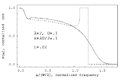
Figure 1: Normalized density of states $N(\omega)$ vs normalized frequency $\omega/(W/2)$ in an electronic band renormalized by the interaction with Einstein oscillator of normalized frequency $\Omega=0.1$. Shown are the results of self-consistent (solid curve) and non self-consistent (dashed curve) calculations for the electronic self energy. The mass enhancement parameter is $\lambda=2$, normalized temperature is $t=0.02$.

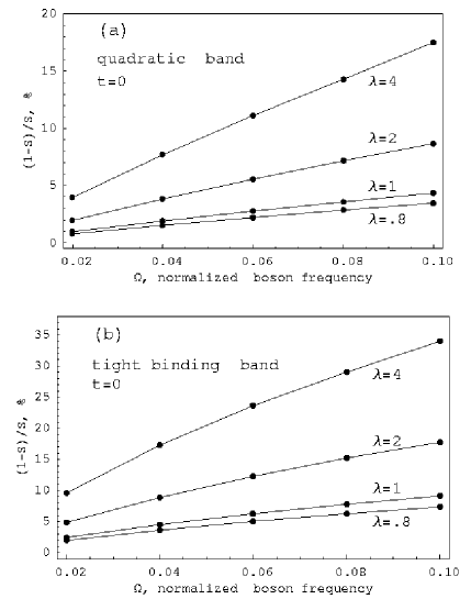
Figure 2: Percent deviation from $1$ of the optical sum as a function of normalized boson frequency $\Omega$ for several values of the mass enhancement parameter $\lambda$. The optical sum deviation from 1 is negative in all cases although here we quote the percentage as a positive quantity. Results are shown for (a) quadratic dispersion and (b) tight binding dispersion. The curves in panel (b) also represent the change in the kinetic energy, irrespective of the above choice of the band structure.

III Discussion of the results

For purposes of presentation, we show results for the optical integral $S$ in dimensionless form, i.e. by omitting the factor that precedes the square brackets in Eq. (8) for the quadratic dispersion, and in Eq. (11) for the tight-binding dispersion. Thus, the ‘standard’ value for the sum rule in the ensuing results corresponds to a value 1. All energies are measured in units of $W/2$, half of the bare electronic bandwidth. We also use normalized variables: the normalized frequency of Einstein oscillators, $\Omega\equiv\omega_{E}/(W/2)$, the normalized temperature, $t\equiv T/(W/2)$, and the normalized area under $\alpha^{2}F(\omega)$, $a\equiv A/(W/2)$.

In Fig. 2 we show zero temperature results for the percent deviation of the total optical spectral weight which results from interactions, i.e. from a finite value of the parameter $a$ which enters the electron boson spectral density. In all cases the deviations are negative but they are plotted as positive as a function of the normalized boson frequency, $\Omega$. The top (bottom) frame applies to the case with quadratic (tight-binding) dispersion. The various curves are labeled by the value of electron mass enhancement parameter $\lambda$ that were used. We see that for a fixed value of $\lambda$ the percent deviation increases as $\omega_{E}$ increases; similarly, for fixed $\omega_{E}$ and increasing $\lambda$ the deviation increases. While both band structure models show the same qualitative behavior the effect is larger for the tight binding case. Note that the result in the lower frame also represents the kinetic energy change. The optical sum and the kinetic energy do follow each other but are numerically different for the quadratic band case.

In Fig. 3 we consider temperature variations of the optical sum as a function of normalized temperature $t$. Results for $a=0.02$ (top frame) and $a=0.1$ (bottom frame) are shown. The former value corresponds to conventional metals while the latter number is characteristic of strongly coupled systems like the high–T_c cuprates. For Fig. 3 we have chosen two representative values of the boson frequency $\omega_{E}$: in the top frame they correspond to $\lambda=0.8$ and $1$, while in the bottom frame they correspond to $\lambda=2$ and $4$. In both frames we show the optical sum derived from both the quadratic band and the tight binding band, as indicated. In each frame solid and dashed curves are used to distingush between the results for two different values of the electron enhancement parameter. We see that, with $a$ and $\lambda$ parameters fixed, the temperature variations of the optical sum for tight binding are larger than for quadratic bands.

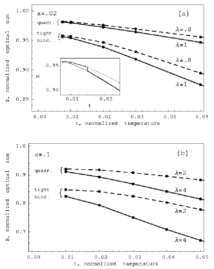
Figure 3: The variation of the optical sum vs. temperature for the interaction strengths (a) $a=0.02$ and (b) $a=0.1$. The results are for both the quadratic and tight binding band, as indicated. In panel (a) the mass enhancement parameter $\lambda=0.8$ (dashed curves) and $\lambda=1$ (solid curves), while in panel (b) $\lambda=2$ (dashed curves) and $\lambda=4$ (solid curves). The insert in panel (a) illustrates the behavior of the optical sum during a sudden “undressing transition” at $t_{undress}=0.02$ with 20% hardening of the normalized boson frequency $\Omega$ and a corresponding reduction of the the mass enhancement parameter from $\lambda=1.0$  to $\lambda=0.8.$

In all cases the variation of the optical sum with temperature increases as $\lambda$ increases. At the same time the absolute value of the deviation of $S$ from 1 at $t=0$ increases with increasing coupling strength $a$ (compare the top frame with the bottom frame). This is in accordance with the results presented in Fig. 2 where we see that for a fixed $\lambda$ the absolute value of the deviation grows as $\Omega$ increases (remember that $a=\lambda\Omega/2$).

From Fig. 3 we conclude that interactions play an essential role in determining the temperature dependence of the optical sum. To understand this point better we return to Eq. (2) which gives the optical sum as an integral of two factors, the second derivative of the electron dispersion, and the occupation probability, $n(\xi_{k})$, given by Eq. (6). The temperature dependence of $n(\xi_{k})$ derives from two sources: the Fermi function $f_{F}\left(\omega\right)$ and the electron spectral function $A\left(\xi,\omega\right)$. The former factor is always operative, even in the noninteracting case. The latter factor produces an additional temperature dependence only when self energy effects are included (check Eqs. (12)–(13) which include temperature through the functions $f_{F}\left(\omega\right)$ and $f_{B}\left(\omega\right)$).

To get some idea of the significance of this second source of the temperature dependence we evaluate Eq. (6) with the thermal factor $f_{F}\left(\omega\right)$ artificially ”switched off” and kept in the form valid at $t=0$ (i. e. in the form of the step function), but with the spectral function $A\left(\xi,\omega\right)$ evaluated properly from Eqs. (12)–(13) for a range of temperatures. The results are shown in Fig. 4a for $t=0.0,0.01,0.03$ and $0.05$. Sharper curves correspond, of course, to lower temperatures. We see that the temperature dependence of $n(\xi)$ obtained in this way is quite strong.

The full temperature dependence of the occupation probability $n(\xi)$, resulting when both the thermal factor $f_{F}\left(\omega\right)$ and the temperature dependence of $A\left(\xi,\omega\right)$ are accounted for in Eq. (6), is illustrated in Fig. 4b by dashed curves. We have also included the corresponding results from Fig. 4a so a direct comparison could be made. The conclusion is that the temperature dependence of the self energy is always important for determining the occupation probability $n_{k}(T)$ and therefore plays an essential role in the sum rule. This source of the temperature dependence of $S$ becomes dominant as the temperature increases. This important dependence is omitted in Ref. vdmarel2 ; in that analysis interactions were not included.

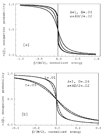
Figure 4: The probability of occupation of the state $n(\xi)$ vs normalized energy $\xi/(W/2)$. (a) The results for the case when only the temperature dependence of the self energy is included. The normalized temperatures are $t=0.0,0.01,0.03$ and $0.05$, with broader curves corresponding to higher temperatures. (b) Comparison of the results when the complete temperature dependence of $n(\xi)$ (see Eq. (6)) is accounted for (dashed curves) with the case presented in (a) (solid curves). The normalized temperatures are $t=0.01$ and $0.05$, as indicated.

Figure 5: The percent variation in the optical sum between normalized temperatures $t=0.025$ and $t=0$ vs. the normalized boson frequency $\Omega$ for the values of mass enhancement parameter $\lambda=0.8,1,2$, and $4$. Panel (a) applies to the parabolic band, and panel (b) to the tight binding band. The dashed line shows the 2% loss of $S$ estimated from the data of Molegraaf et al vdmarel1 .

In Fig. 5 we show the percentage spectral weight lost between $t=0$ and $t=0.025$ as a function of the normalized boson energy $\Omega$ for several values of the mass enhancement parameter $\lambda$. We see that the percentage increases with increasing $\lambda$ but that for a fixed $\lambda$ it decreases with increasing values of $\omega_{E}$ in the range of parameters considered. In a recent experiment Molegraaf et al vdmarel1 have found that the optical sum decreases noticeably from $0$ K to $200$ K in two cuprate superconducting samples. From the data in this reference we estimate the corresponding percentage change to be of the order of 2%. We show this as a horizontal dotted line in Fig. 5. Note that in these experiments the bandwidth $W$ is estimated to be 1.25 eV and $T=200$ K corresponds to $t=.027$, close to the value used in Fig. 5. While our theory is simple with coupling to a single boson only, the experimental observation puts a constraint on allowed values of $\Omega$ and $\lambda$. Only those results that fall close to the dotted line are possible. This still leaves a considerable range of possible parameters. If one has in mind a particular boson model such as phonons or spin fluctuations, $\omega_{E}$ is further constrained and the optical sum rule can be used to deduce the value of $\lambda$. Alternatively, from a detailed fit to the frequency dependence of the optical conductivity in the cuprates, Schachinger and Carbotte carbotte-book have determined that $\lambda\simeq 2$ in these materials. Reference to the lower frame of Fig. 5 gives an estimate of $\Omega\approx 0.1$, This implies a frequency $\omega_{E}\approx 62$ meV, which is somewhat high for phonons. Extensive calculations carbotte-rmp  for a distributed electron–boson spectra $\alpha^{2}F(\omega)$ suggest that the appropriate single frequency characterizing the spectrum is $\omega_{\ln}$, which is equal to approximately one half of the maximum phonon energy ($\omega_{D}$). For the cuprates this should be $\lesssim 40\,$ meV.

We will not pursue this point here note , but instead focus on the primary observation of Molegraaf and coworkersvdmarel1 . They find an abrupt jump upwards in the optical spectral weight as the temperature is lowered into the superconducting state in two cuprate materials. They interpret this as indicative of a decrease in the absolute value of the kinetic energy. This is contrary to what is expected in the conventional BCS framework and is suggestive of a novel type of kinetic energy driven superconductivity. Returning to the top frame of Fig. 3 note that if at a critical temperature $T_{c}$ a phase transition occurs in which the boson energy hardens (leaving everything else the same) so that $\lambda$ changes from 1.0 to 0.8 say, the corresponding total optical spectral weight would jump from the solid to the dashed line. This is illustrated in the inset. ‘Undressing’ of the electron’s mass due to hardening of the boson spectrum leads directly to an increase in the optical sum and a decrease in the kinetic energy. We have not considered specifically the superconducting transition. In this case the reduction in kinetic energy due to the undressing process would have to overcompensate for the increase in kinetic energy that occurs when Cooper pairs form. Schachinger, Carbotte and Basov carbotte1 (see also reference carbotte-book ) have determined the boson spectrum involved for electron interactions in the cuprates from considerations of the frequency dependence of the infrared conductivity. They found that, as the temperature is reduced, the boson spectrum becomes gapped at low frequency with formation of an optical resonance at higher frequency, a process which effectively corresponds to a hardening of the boson spectrum; this change would manifest itself as the ‘undressing’ process described here. A similar conclusion was reached in Ref. haslinger03 based on calculations of the condensation energy.

IV Conclusions

We have adopted a very simple model for interacting electrons to investigate the dependence of the optical sum on interactions and temperature. The model consists of electrons with bandwidth $W$ with a constant density of states, and with a dispersion given by either a parabolic relation or a tight-binding description. This additional modelling is required for the dispersion in order to correctly describe the group velocity, whose energy dependence is important for satisfying the optical sum rule. These electrons interact with a boson, and we have described this interaction with a (self-consistent) Migdal approximation. The optical conductivity is described by the bubble approximation; one can readily verify that the optical sum rule, which relates an exact two particle response function to an exact single particle property, is satisfied by these two (seemingly) unrelated approximations.

A natural interpretation of the sum rule experiments vdmarel1 ; lobo1 ; vdmarel2 ; hirsch3 is to infer a novel mechanism for superconductivity that is accompanied by a kinetic energy decrease (absolute value), in contrast to the usual BCS case. Here we have adopted an approach which in this sense is conventional; the deviation from the usual BCS case instead arises because of a change in the boson characteristics at and below the superconducting transition. This possibility was inspired by an analysis of the neutron scattering data which showed a definite change in the spin fluctuation spectrum at $T_{c}$ carbotte-book ; carbotte1 . Here we have modelled these changes as a shift in boson spectral weight from low to high frequency with a concomitant lowering of $\lambda$. As our results show, this leads naturally to an increase in the optical sum, as observed in experiment. Thus, these experiments, along with others carbotte-book ; carbotte1 ; timusk04 find a consistent explanation in boson mediated superconductivity accompanied by temperature dependent changes in the boson spectral function.

V Acknowledgments

Work supported by the Natural Science and Engineering Research Council of Canada (NSERC) and the Canadian Institute for Advanced Research (CIAR).

References

- (1) H.J.A. Molegraaf, C. Presura, D. van der Marel, P.H. Kes, and M. Li, Science 295, 2239 (2002).
- (2) A.F. Santander-Syro, R.P.M.S. Lobo, W. Bontemps, Z. Konstantinovic, Z.Z. Li, and H. Raffz, Europhys. Lett. 62, 568 (2003).
- (3) C.C. Homes, S.V. Dordevic, D.A. Bonn, Ruixing Liang, and W.N. Hardy, cond-mat/0303506.
- (4) D. van der Marel, H.J.A. Molegraaf, C. Presura, and I. Santoso, cond-mat/0302169.
- (5) A.E. Karakozov, E.G. Maksimov, and O.V. Dolgov, cond-mat/0208170.
- (6) J.E. Hirsch, Physica C 199, 305 (1992); Physica C 201, 347 (1992).
- (7) J.E. Hirsch and F. Marsiglio, Phys. Rev. B62, 15131 (2000).
- (8) J.E. Hirsch, Science 295, 2226 (2002).
- (9) D.N. Basov et al, Science 283, 49 (1999).
- (10) A.S. Katz et al, Phys. Rev. B61, 5930 (2000).
- (11) Wonkee Kim and J.P. Carbotte, Phys. Rev. B64, 104501 (2001); Phys. Rev. B61, R11886 (2000); Phys. Rev. B63, 140505(R) (2001).
- (12) S. Chakravarty, Euro. Phys. J, B5, 337 (1998).
- (13) P.W. Anderson, in The Theory of Superconductivity in the High-Tc Cuprates, Princeton University Press, Princeton, N.Y. (1998).
- (14) M.R. Norman and C. Pepin, Phys. Rev. B66, 100506 (2002).
- (15) M.R. Norman and C. Pepin, cond-mat/0302347.
- (16) S. Engelsberg and J.R. Schrieffer, Phys. Rev. 131, 993 (1963).
- (17) A.S. Alexandrov, V.N. Grebenev, and E.A. Mazur, Pis’ma Zh. Eksp. Teor. Fiz. 45 357 (1987) [JETP Lett. 45 455 (1987)].
- (18) C. Grimaldi, E. Cappelluti, and L. Pietronero, Europhys. Lett. 42, 667 (1998); Phys. Rev. B 64, 125104 (2001).
- (19) E. Cappelluti and L. Pietronero, cond-mat/0309080.
- (20) F. Doğan and F. Marsiglio, Phys. Rev. B68, 165102, (2003).
- (21) F. Marsiglio and J.P. Carbotte, in The Physics of Superconductors: Vol. I, Conventional and High-Tc Superconductors, eds. K.H. Bennemann and J.B. Ketterson, Springer, Berlin (2003), pp.233-345.
- (22) A. Knigavko and F. Marsiglio, Phys. Rev. B 64, 172513 (2001).
- (23) F. Marsiglio, M.Schossmann, and J.P.Carbotte, Phys. Rev. B 37, 4965 (1988).
- (24) F. Marsiglio and J.E. Hirsch, Phys. Rev. B 41, 6435 (1990); F. Marsiglio and J.E. Hirsch, Physica C 165, 71 (1990).
- (25) B. Mitrović and J.P. Carbotte, Can. Jour. Phys. 61, 758 (1983); Can. Jour. Phys. 61, 784 (1983).
- (26) A. Knigavko and J. P. Carbotte, unpublished.
- (27) E. Schachinger and J.P. Carbotte, in Models and Methods of HTC Superconductivity, eds. J.K. Srivastava and S.M. Rao, Nova Scientific, Hauppauge N.Y. (2003); p. 73, Vol. 2.
- (28) J.P. Carbotte, Rev. Mod. Phys. 62, 1027 (1990).
- (29) E. Schachinger, J.P. Carbotte and D.N. Basov, Europhys. Lett. 54, 380 (2001).
- (30) R. Haslinger and A.V. Chubukov, Phys. Rev. B67, 140504(R) (2003).
- (31) J. Hwang, T. Timusk and G.D. Gu, Nature 427 714 (2004).