Charge and spin conductance through a side-coupled quantum dot

Abstract

The zero-temperature magnetic field-dependent conductance of electrons through a one-dimensional non-interacting tight-binding chain with an interacting side dot is reviewed and analized further. When the number of electrons in the dot is odd, and the Kondo effect sets in at the impurity site, the conductance develops a wide minimum as a function of the gate voltage, being zero at the unitary limit. Application of a magnetic field progressively destroys the Kondo effect and, accordingly, the conductance develops pairs of dips separated by $U$, where $U$ is the repulsion between two electrons at the impurity site. Each one of the two dips in the conductance corresponds to a perfect spin polarized transmission, opening the possibility for an optimum spin filter. The results are discussed in terms of Fano resonances between two interfering transmission channels, applied to recent experimental results, and compared with results corresponding to the standard substitutional configuration, where the dot is at the central site of the non-interacting chain.

I Introduction

In recent decades the electric transport through quantum dots (QD) has been extensively studied both theoretically and experimentally mesoscopic1 ; mesoscopic2 ; mesoscopic3 . As the result a comprehensive picture of a big variety of underlying physical phenomena has emerged (See e.g. Areview ; ABGreview and references therein). As QD’s are small droplets of electrons confined in the three spatial directions, energy and charge quantization, and strong Coulomb repulsion among the electrons results from this confinement. As these features are shared with real atomic systems, from the very beginning an extremely useful analogy has been exploited between “real” and “artificial” atomic systems. This analogy received strong support through an experimental breakthrough where the Kondo effect in quantum dots was unambiguously measured.david ; sara ; schmid Historically, the Kondo effect was introduced more than forty years ago to explain the resistivity minimum for decreasing temperatures observed in metallic matrices with a minute fraction of magnetic impurities.jun According to the detailed microscopic theory, when the temperature $T$ decreases below the Kondo temperature $T_{K}$, each of the localized magnetic impurities starts to interact strongly with the surrounding electronic cloud, which finally results in a singlet many-body ground state, reaching its maximum strength at $T=0.$hewson The minimum in the resistivity results from the fact that, as the temperature is lowered, the scattering with phonons decreases down to a temperature at which the scattering with localized impurities becomes important as the Kondo effect starts being operative. It is important to emphasize that in this case, the so-called traditional Kondo effect, magnetic impurities act as scattering centers, increasing the sample resistivity.

The opposite behavior is found in some circumstances in the Kondo effect in quantum dots. The situation considered almost without exception both theoretically and experimentally, consists of a quantum dot connected to two leads in such a way that electrons transmitted from one electrode to other should necessarily pass through the quantum dot (a substitutional dot). As theoretical calculations predicted,glazman ; patrick in this configuration and when the dot is occupied by an odd number of electrons, the conductance increases when decreasing the temperature and the Kondo effect sets in, essentially due to a resonant transmission through the so-called Kondo resonance which appears in the local density of states at the dot site at the Fermi level of the leads. In this situation, at $T=0$, the conductance should take the limiting value $2e^{2}/h,$ corresponding to the unitary limit of a one-dimensional perfect transmission channel.wiel At finite temperatures $T>T_{K}$ the Kondo effect is destroyed and only the standard Coulomb blockade remainsKMMTWW ; AL , which manifests itself in strong oscillations of the dot’s conductance versus the gate voltage applied to the dot.

The aim of this work is to theoretically review the results for an alternative configuration of a side-coupled quantum dot, attached to a perfect quantum wire. In this case, the quantum dot acts as a scattering center for transmission through the chain, in close analogy with the traditional Kondo effect. We have found that when the dot provides a resonant energy for scattering, the conductance has a sharp decrease, reminiscent of the Fano resonances observed in scanning tunneling microscope experiments for magnetic atoms on a metallic substrate.li and QD’s coupled sideways to a quantum wirekoba . A similar problem has been discussed by other authorskang ; aligia ; franco . We differ from them in that they have used approximate methods to describe the Kondo regime (slave-boson mean field theorykang , interpolative perturbation schemealigia and X-slave-boson treatmentfranco ),while our numerical results take into account the many body interactions in a very precise and controlled way. In addition, in Ref. kang they use the unrealistic limit of infinite Coulomb repulsion for electrons inside the dot $($Hubbard $U\rightarrow\infty)$, loosing key features as the double dip structures of Fig. 8a, which give rise to the diamond-shaped features in differential conductance experiments.gores Also in recent years, several authors have studied the possibility of spin polarization in transport through substitutional QD’s costi ; recher ; ohno and other nanoscopic configurations like rings popp , T-shaped spin filters kiselev and dots connected to Luttinger liquid leadsschmeltzer03 . We discuss here that if the spin degeneracy is lifted, say, by an applied magnetic field, and if the splitting exceeds the temperature, the resonances for spin up and spin down electrons become well separated in the absence of the Kondo effect for the case of side-coupled quantum dots. This gives rise to the resonant spin polarized conductance due to the effect of Fano interference. This review is mainly based in results presented by the authors in Refs.torio1 and torio2 .

II The model

The models employed in the calculation are schematically shown in Fig. 1. Case a), corresponding to the substitutional dot situation, consists of two semi-infinite non-interacting tight-binding chains connected to a central site (the dot). Case b), corresponding to the side dot, consists of a quantum wire coupled sideways to a QD. In both cases the dot is modeled as an Anderson impurityanderson . For the linear response situation, $\mu_{L}\rightarrow 0^{+}$ and $\mu_{R}\rightarrow 0^{-}$, the Hamiltonian reads:

$$H=H_{0}+H_{int},$$ (1)

where $H_{0}$ is the Hamiltonian of two semi-infinite chains with site energies all set equal to zero,

$$H_{0}=-\sum_{j,\sigma}t_{j}(c_{j\sigma}^{\dagger}c_{j+1\sigma}+\text{h.c.}),$$ ()

with $j$ running over all chain sites. Here $c_{j\sigma}^{\dagger}$ $(c_{j\sigma})$ represents a creation (destruction) operator for an electron at site $j$ with spin $\sigma,$ and $t_{j}$ are the hopping amplitudes between first-neighbour sites. $H_{int}$ can be written as

$$H_{int}^{a}=\sum_{\sigma}\left(\varepsilon_{\sigma}+\frac{U}{2}\text{ }n_{0\overline{\sigma}}\right)n_{0\sigma},$$ ()

for the substitutional dot configuration, while

$$H_{int}^{b}=\sum_{\sigma}\left[-t_{i}(c_{0\sigma}^{\dagger}c_{\sigma}+\text{h.c.})+\varepsilon_{\sigma}\text{ }c_{\sigma}^{\dagger}c_{\sigma}+\frac{U}{2}\text{ }n_{\sigma}n_{\overline{\sigma}}\right],$$ ()

for the side dot configuration. In the equations above, $\varepsilon_{\sigma}$ represents the energy at the dot site, $U$ $(>0)$ is the Coulomb repulsion energy which penalizes the double occupancy of the dot site, and $t_{j}=t$ for $j\eqslantless-2$, $j\geqslant 1,$ while $t_{-1}=t_{0}=t^{\prime}$, $n_{0\sigma}=c_{0\sigma}^{\dagger}c_{0\sigma}$ and $n_{\sigma}=c_{\sigma}^{\dagger}c_{\sigma}$. As we are also interested in the behavior in a magnetic field, we consider the local energies as $\varepsilon_{\uparrow}=\varepsilon_{0}+\Delta/2,$ $\varepsilon_{\downarrow}=\varepsilon_{0}-\Delta/2,$ with $\Delta=g\mu_{B}H$ the Zeeman splitting of the localized orbital, i.e. the principal magnetic field effect is to shift the local QD levels.meir2 In the usual experimental setup, $\varepsilon_{0}$ can be controlled through application of a gate voltage. It is interesting to point out that both models could be mapped to a single semi-infinite chain, with the dot sitting at the free end, and the remaining sites corresponding to the even basis states that couples to the dot. Both models become exactly equivalent from the point of view of their equilibrium properties,schlott if the hoppings are related as follows: $t_{i}=\sqrt{2}t^{\prime}=t.$ However, the transport properties of both models are completely different. We will set $t=t_{i}1$.

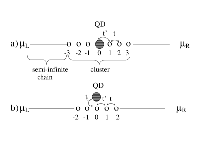
Figure 1: Schematic representation of our models: a) substitutional dot configuration; b) side dot configuration. Small open circles represent cluster non-interacting sites, big full circle represent the dot site. The cluster includes the dot and a few non-interacting sites. Left and right full lines represent the non-interacting tight-binding semi-infinite chains with their respective chemical potentials $\mu_{L}$ and $\mu_{R}$.

For the analysis of our transport results we have used the following equation for the magnetic field dependent conductance,meir

$$g(H)=\sum_{\sigma}g_{\sigma}(H)=\frac{e^{2}}{h}\frac{2\pi t^{\prime}{}^{2}}{t}\sum_{\sigma}\rho_{\sigma}(\varepsilon_{F})$$ ()

where $\rho_{\sigma}(\varepsilon_{F})$ is the local density of states (per spin) at site $0$ evaluated at the Fermi energy $\varepsilon_{F}.$ To obtain the density of states $\rho_{\sigma}(\varepsilon_{F})$ in a general interacting case $(U\neq 0)$ we use a combined method. In the first place we consider an open finite cluster of $N$ sites in the projected space ($N=7$ in our case) which includes the impurity. This is diagonalized using the exact diagonalization Lanczos techniquelanczos . We then proceed to embed the cluster in an external reservoir of electrons, which fixes the Fermi level of the system, attaching two semi-infinite leads to its right and leftferrari . This is done by calculating the one-particle Green function $\hat{G}$ of the whole system within the chain approximation of a cumulant expansioncumulant for the dressed propagators. This leads to the Dyson equation $\hat{G}=\hat{G}\hat{g}+\hat{T}\hat{G}$, where $\hat{g}$ is the cluster Green function obtained by the Lanczos method. Following Ref. ferrari , the charge fluctuation inside the cluster is taken into account by writing $\hat{g}$ as a combination of $n$ and $n+1$ particles with weights $p$ and $1-p$ respectively: $\hat{g}=p\hat{g}_{n}+(1-p)\hat{g}_{n+1}$. The total charge of the cluster $Q_{c}$ and $p$ are calculated by solving selfconsistently the equations:

$$Q_{c} = np+(n+1)(1-p),$$ ()

$$Q_{c} = -\frac{1}{\pi}\int_{-\infty}^{\varepsilon_{F}}\sum_{i}\text{Im }g_{ii}(\omega)\text{ }d\omega,$$ ()

where $i$ runs on the cluster sites. Once convergence is reached, the density of states is obtained from $\hat{G}$. It is important to stress that this method is reliable only if $t^{\prime}$ (substitutional dot) or $t_{i}$ (side dot) are large enough, so that the Kondo cloud is about the size of the cluster (for the parameters used here we estimate a Kondo correlation lenght of about 10 lattice sites). Moreover, the fact that the conductance reaches the unitary limit for the symmetric case provides an important test of the validity of the method (see Fig. 9).

III Single particle $(U=0)$ Fano resonance

Let us consider first the case $U=0,$ where an analytical and instructive calculation of $g_{\sigma}$ is feasible, along the following lines. For this non-interacting situation, the conductance per spin channel $g_{\sigma}$ is linked to the transmission amplitude $\tau_{\sigma}$ by the Landauer formula

$$g_{\sigma}=\frac{e^{2}}{h}|\tau_{\sigma}|^{2}.$$ ()

Comparison with Eq.(5) above yields a Fisher-Lee type of relation $\left[2\pi(t^{\prime})^{2}/t\right]\rho_{\sigma}(\varepsilon_{F})=|\tau_{\sigma}|^{2}.$FL For the side-dot configuration of Fig. 1b the transmission can be computed within the one-particle picture for an electron moving at the energy $\varepsilon$ :

$$-\varepsilon\phi_{j,\sigma}=t(\phi_{j-1,\sigma}+\phi_{j+1,\sigma})+(t^{\prime}-t)(\delta_{j,1}+\delta_{j,-1})\phi_{0,\sigma},\hskip 14.22636ptj\neq 0$$ (2)

$$-\varepsilon\phi_{0,\sigma}=t^{\prime}(\phi_{-1,\sigma}+\phi_{+1,\sigma})+t_{i}\varphi_{\sigma},$$ ()

$$-\varepsilon\varphi_{\sigma}=-\varepsilon_{\sigma}\varphi_{\sigma}+t_{i}\phi_{0,\sigma},$$ ()

where $\delta_{i,j}$ is the Kronecker symbol, $\phi_{j,\sigma}$ refers to the spin-dependent amplitude of a single particle at site $j$ in the conducting channel, and $\varphi_{\sigma}$ is the amplitude at the side dot. The scattering problem is solved by the ansatz

$$\phi_{j<\text{ }0,\sigma}=e^{iqj}+\rho_{\sigma}\text{ }e^{-iqj},\qquad\phi_{j>\text{ }0,\sigma}=\tau_{\sigma}\text{ }e^{iqj},$$ ()

with the usual dispersion relation $\varepsilon=-2t\cos q{,}$ $\rho_{\sigma}$ and $\tau_{\sigma}$ being the spin-dependent amplitudes for reflexion and transmission through the impurity region, respectively. Substituting Eq. (12) in Eqs. (9-11) we readily find

$$\tau_{\sigma}=\frac{\left[2i(t^{\prime})^{2}/t\right]\sin q}{\left[2i(t^{\prime})^{2}/t\right]\sin q+\varepsilon\left[(t^{\prime}/t)^{2}-1\right]+t_{i}^{2}(\varepsilon_{\sigma}-\varepsilon)^{-1}},$$ ()

hence the conductance

$$g_{\sigma}=\frac{e^{2}}{h}|\tau_{\sigma}|^{2}=\frac{e^{2}}{h}\left\{1+\frac{t^{2}}{4(t^{\prime})^{4}\sin q}\left[\frac{\varepsilon}{t^{2}}(t^{\prime\text{ }2}-t^{2})+\frac{t_{i}^{2}}{(\varepsilon_{\sigma}-\varepsilon)}\right]^{2}\right\}^{-1}.$$ ()

For $t^{\prime}=t$ and $\varepsilon$ equal to the Fermi energy $\varepsilon_{F},$ which is the only energy that matters in the linear response regime, Eq.(14) reduces to the simpler expressiontorio2

$$g_{\sigma}=\frac{e^{2}}{h}\left[1+\frac{(\Gamma/2)^{2}}{(\varepsilon_{\sigma}-\varepsilon_{F})^{2}}\right]^{-1},$$ ()

where $\Gamma=t_{i}^{2}/t=2t_{i}^{2}/\left|v_{F}\right|,$ with $\left.v_{F}=d\varepsilon/dq\right|_{q_{F}}$ is the Fermi velocity, and $q_{F}$ the Fermi wave-vector. As a function of $\varepsilon_{\sigma},$ $g_{\sigma}=0$ if $\varepsilon_{\sigma}=\varepsilon_{F},$ and reaches a value close to the unitary limit $e^{2}/h$ if $\left|\varepsilon_{\sigma}-\varepsilon_{F}\right|\gg\Gamma/2.$ The associated valley in the conductance has a typical width of about $\Gamma.$

On the other hand the mean occupation number on the dot at zero temperature $\left\langle n_{\sigma}\right\rangle$ is related to the scattering phase shift by the Friedel sum rule hewson ; langreth

$$\left\langle n_{\sigma}\right\rangle=-\frac{1}{\pi}{\rm{Im}\;\ln{(}}\varepsilon_{F}-\varepsilon_{\sigma}+i\Gamma/2{),}$$ ()

which combined with Eq.(15) yields the relation

$$g_{\sigma}=\frac{e^{2}}{h}\cos^{2}(\pi\left\langle n_{\sigma}\right\rangle).$$ ()

This relation has a geometric origin and actually holds for arbitrary $U$ provided zero temperature limit. This is in contrast to Eqs. (13,14,15) which are applicable only for $U=0$.

We display in the upper panel of Fig. 2 the dot occupancy $\left\langle n_{\sigma}\right\rangle$ as a function of the resonant level energy $\varepsilon_{0}.$ From here on, we set $\varepsilon_{F}=0,$ corresponding to a mean occupancy of one for each of the chain sites. As expected, $\left\langle n_{\sigma}\right\rangle$ changes from a value close to unity for $\varepsilon_{0}\ll 0$, to a value close to zero for $\varepsilon_{0}\gg 0$, passing through $\left\langle n_{\sigma}\right\rangle=1/2$ for $\varepsilon_{0}=0.$ The lower panel of Fig. 2 corresponds to the conductance $g_{\sigma},$ whose more noticeable feature is that it is zero for $\varepsilon_{0}=0,$ meaning that the transmission through the chain is extremely small in this regime. This is the first example of a Fano resonance discussed in this work; as $t_{i}=t=1,$ the width of the resonance $\Gamma/t\simeq 1.$ The symmetric form of the Fano resonance given by Eq. (15) is based on the symmetry of the coupling term in the Hamiltonian (1). Fig. 3 corresponds to the results with a magnetic field, parametrized by $\Delta/t=1.6.$ The magnetic field breaks the dot energy degeneracy, $\varepsilon_{\uparrow}\neq\varepsilon_{\downarrow},$ and the dot occupancy $\left\langle n_{\sigma}\right\rangle$ depends on spin. The conductance becomes also spin-dependent, as displayed in the lower panel of Fig. 3. For strong magnetic fields $\left(\Delta\gg\Gamma\right),$ the two Fano resonances for spin up and spin down electrons are energetically well separated. Therefore, the current through the channel is completely polarized at $\varepsilon_{\uparrow}=\varepsilon_{F}$ and $\varepsilon_{\downarrow}=\varepsilon_{F}$. For example, for $\varepsilon_{0}=-\Delta/2,$ $g_{\uparrow}=0$ while $g_{\downarrow}$ $\simeq e^{2}/h,$ leading to a perfect spin blocking for electrons with spin $\uparrow.$ The situation reverses for $\varepsilon_{0}=\Delta/2.$

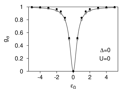
Figure 2: Mean dot occupation $\langle n_{\sigma}\rangle$ (top) and the channel conductance $g_{\sigma}$ (bottom) in units of $[e^{2}/h]$ versus the resonance energy $\varepsilon_{0}$ for zero magnetic field and $U=0$. The results computed numerically by different means are: using Eq. (5) (white dots); using $\left\langle n_{\sigma}\right\rangle$ and Eq. (17) (black dots). Solid line: mean occupation and conductance obtained from the exact solution by Wiegmann and Tsvelick WT .

IV Many-body $(U\neq 0)$ Fano resonances

IV.1 Weak magnetic field $(\Delta\ll k_{B}T_{K})$

We will first consider the case of zero magnetic field $\Delta=0$ but finite Coulomb interaction $U$. For zero side-dot/chain coupling $t_{i}=0$, the single particle excitations on the dot are located at energies $\varepsilon_{0}$ and $\varepsilon_{0}+U$. When the dot is weakly connected to the conducting channel (and at very low temperatures, $T<T_{K}$), a resonant peak in the density of states on the dot arises at the Fermi energy due to the Kondo effect. By using an approach identical to that of Refs. glazman ; patrick , we conclude that the channel conductance $g_{\sigma}$ is controlled entirely by the expectation value of the particle number $\langle n_{\sigma}\rangle$ as given by Eq. (17)torio2 . This reasoning justifies Eq. (17) for any values of $U$ and $\Delta$ kang-remark . Note that in the standard setup of the substitutional configuration the dot’s conductance is proportional to $\sin^{2}(\pi\langle n_{\sigma}\rangle)$ glazman ; patrick ; langreth due to the different geometry of the underlying system.

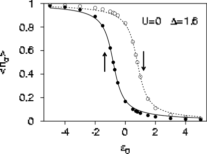
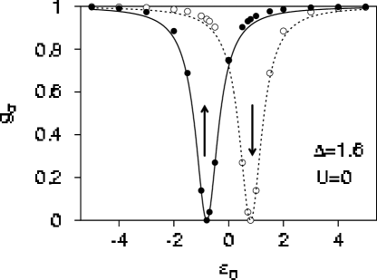
Figure 3: Same as Fig. 2 for a finite splitting $\Delta=1.6$ and $U=0$. The black (white) dots represent the numerical results for the spin up (spin down) occupation number. The solid and dotted lines represent the exact results of Eqs. (16) (upper panel) and (15) (lower panel).

In order to compute $\langle n_{\sigma}\rangle$ for finite $U$ we use the numerical techniques developed in Refs. ferrari ; torio1 and summarized above. We compare our results to those obtained from the exact solution for $\langle n_{\sigma}\rangle$ by using the Bethe anzatsWT . The latter holds only for the linearized spectrum (which is not a serious restriction at half-filling) and has a compact form only in the case of zero magnetic field. We plot in the upper panel of Fig. 4 $\langle n_{\sigma}\rangle$ versus the resonance level energy $\varepsilon_{0}$ for $U=12$. In the presence of Coulomb repulsion the mean occupancy of the dot $\langle n_{\sigma}\rangle$ has a flat region near the value $1/2$ due to many-body effects. The physical source of the flat region is as follows. For $U\neq 0,$ the condition for near unity dot occupancy per spin (fully occupied dot regime) is $-(\varepsilon_{0}+U)\gg\Gamma.$ On the other side, the condition for near zero dot occupancy (empty dot regime) is $\varepsilon_{0}\gg\Gamma.$ Accordingly, there is a transition regime, characterized by $0\lesssim\left|\varepsilon_{0}\right|\lesssim U$ where $\langle n_{\sigma}\rangle$ changes from one to zero. Roughly, this is the size of the flat region with $\langle n_{\sigma}\rangle\simeq 1/2$ in the upper panel of Fig. 4. This should be contrasted with the width of this transition regime in the non-interacting case, which is of the order $\Gamma$ (see upper panel of Fig. 2).

The flat region around $\langle n_{\sigma}\rangle=1/2$ for the interacting case translates inmediatly to a valley of width of order $U$ of small channel conductance (see lower panel of Fig. 4). Note that similar results for the limit $U\rightarrow\infty$ have been recently obtained by Bulka and Stefanski bulka01 . In their case, however, instead of a valley, the conductance as a function of $\varepsilon_{0}$ only displays a monotonous increase from the small conductance regime to the high conductance regime, as the fully occupied regime is never reached if $U\rightarrow\infty.$ The conductance found from the numerical evaluation of $\langle n_{\sigma}\rangle$ for finite $U$ is in better agreement with the exact results WT than the conductance computed from Eq. (5). Presumably, the discrepancy originates from finite-size effects (in some cases the Kondo length is larger than the system size used in the numerical computation). The numerical calculation of $\langle n_{\sigma}\rangle$, which involves the energy integration, appears to be more precise than that of the local density $\rho_{\sigma}(\varepsilon_{F})$.

IV.2 Strong magnetic field $(\Delta\gg k_{B}T_{K})$

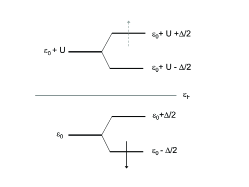
Figure 6: Schematic energy diagram of the interacting side-dot. The full down (dashed up) arrow represents the presence (absence) of an electron with spin down (up).

In the presence of a strong magnetic field such than the Kondo effect is destroyed $(\Delta\gg k_{B}T_{K}),$ the dot occupation for spin up and spin down electrons becomes essentially non-overlaping for a large “window” of values of the resonant energies $\varepsilon_{0}$; this is shown in the upper panel of Fig. 5. The expectation value $\langle n_{\sigma}\rangle$ decreases abruptly from $1$ to $0$ with increasing the resonant energy $\varepsilon_{0}$, but it takes the value $1/2$ at different gate voltages for $\sigma=\uparrow$ and $\sigma=\downarrow$. We will explain this by using the schematic energy diagram of Fig. 6. Note that due to the dot-chain hopping $t_{i},$ each dot discrete level should have a width of about $\Gamma$. For $\varepsilon_{0}\gg\Gamma,$ all dot levels are above the Fermi energy $\varepsilon_{F}(=0),$ the dot is empty, and $\langle n_{\uparrow}\rangle\simeq\langle n_{\downarrow}\rangle\simeq 0.$ When decreasing the gate voltage and $\varepsilon_{0}-\Delta/2=\varepsilon_{F},$ the occupancy of the dot with an electron of spin $\downarrow$ is allowed, and accordingly $\langle n_{\downarrow}\rangle\neq 0,$ $\langle n_{\uparrow}\rangle\simeq 0.$ The important point now is that if $U\neq 0,$ the entrance of the second electron with spin $\uparrow$ is blocked until $\varepsilon_{0}+U+\Delta/2\simeq\varepsilon_{F},$ that is $\varepsilon_{0}\simeq-U-\Delta/2.$ The difference in resonant energy between two events is $U+\Delta$ $(\simeq U).$ On the other side, in the non-interacting case $U=0,$ and the second electron should only overcome a much smaller barrier of size $\Delta$ to be in the dot.

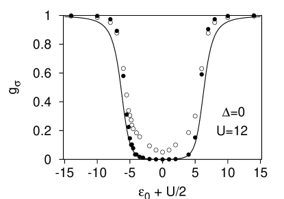
Figure 4: Same as Fig. 2 but for $U=12$

Consequently we may obtain a perfect spin filter as in the case of noninteracting electrons. In Fig. 5 (lower panel), we plot the numerical results for the conductance obtained from Eq. (5) for $U/t=12$ with $\Delta/t=1.6$. Since the dot levels are no longer degenerate the Kondo effect is totally suppressed even at zero temperature. Indeed no plateaus form near $\langle n_{\sigma}\rangle=1/2$ in Fig. 5 (upper panel). As a result the spin-dependent resonances in the conductance have width $\Gamma$. The effect of large $U$ manifests itself mainly in the mere enhancement of the level splitting. Using the common terminology of transport through quantum dots, the results shown in Fig. 5 could be termed as $``$spin-resolved Coulomb blockade dips ”. At low temperatures $T\ll\Delta$ the mean occupation number $\langle n_{\sigma}\rangle$ is close to unity while the occupation number for the opposite spin direction decreases to zero. One can observe, however, from Fig. 5 (lower panel) that there is a mixing of the levels which gives rise to the non-monotonous behavior of $\langle n_{\sigma}\rangle$. This results in a small dip of the spin down conductance at the resonance energy for the spin up electrons and vice versa.

IV.3 Magnetic field quenching of the Kondo-Fano resonance $(\Delta\simeq k_{B}T_{K})$

As a reference for our side-dot results for intermediate magnetic fields $(\Delta\simeq k_{B}T_{K})$, we start by presenting in Fig. 7 the conductance results for the geometrical configuration corresponding to Fig. 1a: the substitutional QD. As discussed above, at zero-temperature and magnetic field, the Kondo resonance which develops right at the Fermi level greatly enhances the transmission when the average dot occupancy is close to 1 (Kondo regime). For the symmetric situation $\varepsilon_{0}=-U/2$, the transmission is perfect and the conductance reaches the unitary limit $g(0)=2e^{2}/h.$wiel This is a highly non-trivial check from the numerical point of view, and proves that our finite system approach is capable of sustaining a fully developed Kondo peak with the exact spectral weight. Within our approach, the Coulomb blockade peaks become discernible upon magnetic field application. As seen in Fig. 7, with increasing magnetic field values, spin-fluctuations at the impurity site are progressively quenched, and the associated enhancement of the conductance develops towards the usually observed experimentally Kondo valley flanked by two Coulomb blockade peaks roughly separated by $U$.

The conductance behaviour equivalent to the traditional Kondo effect, corresponding to the geometrical arrangement of Fig. 1b, is shown in Fig. 8. In this configuration, the conductance reaches the unitary limit either when the dot is fully occupied ($\varepsilon_{0}+U<0$) or empty ($\varepsilon_{0}>0$ ). In both cases, the side dot weakly perturbs the transmission along the tight-binding chain, as the possible scattering processes disappear. On the other side, the conductance becomes progressively blocked as the side dot enters in the Kondo regime, reaching the anti-unitary limit $g(0)=0$ exactly at the side dot symmetric configuration $\varepsilon_{0}=-U/2.$ In other words, even though the non-interacting central site provides, in principle, a channel for transmission, through its coupling to the side dot it becomes a perfectly reflecting barrier. In Fig. 8b we present the conductance for up spins only (spin down conductance shows a behaviour symmetric with respect to the Fermi energy). As expected each channel contributes with $e^{2}/h$ far from the intermediate valence zone (large $|\varepsilon_{0}|$). Comparing with Fig. 8a, we find that within the low conductance regime, the spin discriminated conductance reaches zero for one spin species (up in this case) indicating that for that particular gate voltage the system transmits only the opposite spin and complete reflects the other. This is also seen in the local DOS (see Fig. 10b and comment below). By increasing the magnetic field, and when the Kondo effect is destroyed completely, the separation between up and down conductance dips becomes of the order of the dot interaction energy $U$.

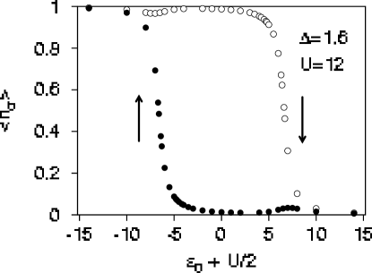
Figure 5: Same as Fig. 3 but for $U=12$

The results for the total ($\rho_{\uparrow}+\rho_{\downarrow}$) local density of states (DOS) shown in Fig. 9 provides a nice qualitative explanation of the linear conductance results in both geometrical arrangements. Fig. 9a corresponds to the local DOS at site 0 in the chain, Fig. 9b to the local DOS at the side dot. Starting with Fig. 9b, a well-defined Kondo resonance is discernible around the Fermi level in absence of magnetic field. The exact (unitary) zero-field result $\sum\limits_{\sigma}\rho_{imp,\sigma}(0)=t/(\pi t^{\prime\text{ }2})=2/(\pi t)\simeq 0.64$ $($for $t=\sqrt{2}t^{\prime}$ and $t=1)$ is recovered from our numerical approach, as discussed above.hewson

This local DOS at the impurity site in the side dot configuration is equivalent to the local DOS at the impurity in the substitutional dot configuration, and gives rise to the unitary limit $g(0)=2e^{2}/h$ discussed above. From the half-width of the zero-field impurity DOS at half-maximum (HWHM), we estimate $k_{B}T_{K}/t\simeq 0.15$ for our parameter choice; note that this estimate qualitatively agrees with the magnetic field values (Zeeman splittings) for which strong dependences of $g(H)$ with $H$ are found. In the presence of a magnetic field, the Kondo resonance splits into two peaks, generating a local minimum between them. As the conductance in the substitutional dot configuration is proportional to the dot DOS at the Fermi level, this explains the abrupt decreasing of $g(H)$ by increasing $H$ at the middle of the Kondo valley shown in Fig. 7. The most noticeable feature of Fig. 9a, corresponding to the DOS at site 0 of the chain, is the profound dip it exhibits around the Fermi level; a pseudo-gap appears at the symmetric situation $\varepsilon_{0}=-U/2$ just at the Fermi level. The presence of this pseudo-gap explains the conductance minimum of Fig. 8 at $\varepsilon_{0}=-U/2.$ In the presence of a magnetic field, the dip weakens and accordingly the conductance starts to increase. After a certain threshold field, the DOS develops a double-well shape around the Fermi level; the distance between the two well minima is about $2\Delta,$ which should be compared with the Zeeman splitting $\Delta.$ If the magnetic field is big enough $(\Delta/k_{B}T_{K}\gg 1)$, the Kondo effect is destroyed, the associated low energy coupling between the quantum wire and the side dot essentially vanishes, and the DOS at site $0$ recovers the semi-elliptical shape corresponding to the non-interacting chain.

In Fig. 10a we show the local DOS at site $0$ in the chain for spins up only for different magnetic fields in the symmetric case. It is clearly seen here that for each field there exists an energy at which the DOS is zero. For down spins the situation is symmetric with respect to zero energy. For large fields the Kondo dips disappear and the dips appear only at the localized energy levels $\varepsilon_{0}-\Delta/2$ and $\varepsilon_{0}+U+\Delta/2$ (not shown). In Fig. 10b the DOS for up spins at site $0$ for the asymmetric case and a small magnetic field is shown. We can see here the evolution of the DOS at the Fermi energy (which defines the behaviour of the conductance). The up spin DOS minimum evolves towards the Fermi energy as we lower the gate voltage from the symmetric case until a particular voltage is reached at which the conductance is zero for this spin species (but finite for the opposite one).

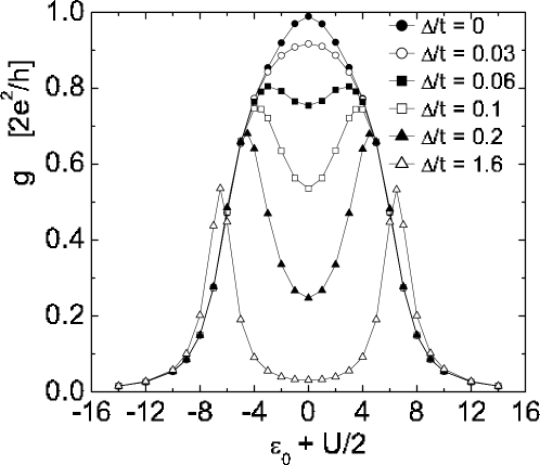
Figure 7: Conductance (in units of $[2e^{2}/h]$) for the substitutional dot configuration, as a function of impurity level position and for several values of the magnetic field ($t^{\prime}/t=1/\sqrt{2}$ and $U=12$).

Conceptually, the simplest way to understand these transport features is using the framework developed by Fano forty years ago.fano He analyzed the properties of a system consisting of a continuous spectrum degenerate with a discrete level, both non-interacting. Under these conditions, a dip develops in the density of states of the continuous spectra, as a result of its interaction with the discrete level. In our case, the continuous spectra is provided by the thigh-binding chain, while the role of the discrete level is played by the Kondo peak at the DOS of the side dot. As the Kondo effect is destroyed by the magnetic field, the intrinsic link discussed above between the Kondo peak and its associated many-body Fano antiresonance implies the weakening of the latter. A most interesting feature of our calculation is the evolution of $g(H)$ for increasing $H$: as the Kondo effect is destroyed, the wide minimum develops a high conductance region around the Fermi level. At high fields, the conductance shows two dips, separated by $U+\Delta.$ These two dips are again quite natural in the Fano framework: in this limit the side dot DOS, has two single-particle resonances at $\omega=\varepsilon_{0}-\Delta/2$ and $\omega=\varepsilon_{0}+U+\Delta/2$ (not shown in Fig. 9b). They give rise to the Coulomb blockade peaks in the substitutional dot configuration: see Fig. 7 at a high magnetic field situation. However, in the side dot configuration, they play the role of two discrete levels which also interfere destructively with the single-particle chain continuum: the result is now two Coulomb dips instead two Coulomb blockade peaks. In light of this analysis, it is clear that the wide dip of Fig. 8 results from the superposition of three quite different dips: a many-body dip around $\varepsilon_{0}=-U/2$ and two single-particle dips around $\varepsilon_{0}=0$ and $\varepsilon_{0}+U=0.$ While our calculation is valid for $T=0,$ it seems reasonable to expect similar qualitative behavior by increasing the temperature: a wide dip (with size $\sim U$) for $T<T_{K},$ two narrow dips (size $\sim\Gamma$) separated by $U$ for $T>T_{K}.$

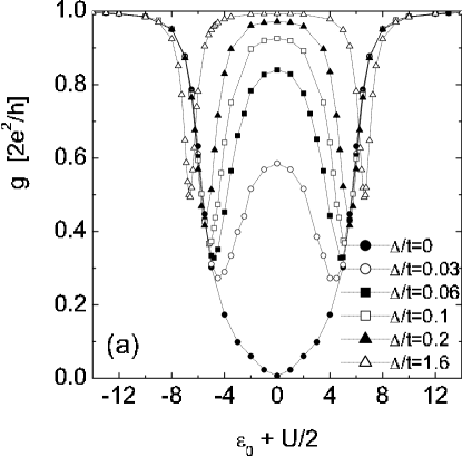
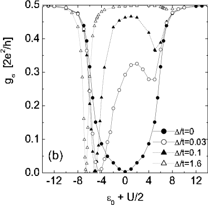
Figure 8: Same as Fig. 7 for the side dot configuration. a) Total conductance; b) conductance corresponding to the spin up channel (note the change in units as compared to Fig. 5). Spin down conductance is symmetric with respect to zero energy.

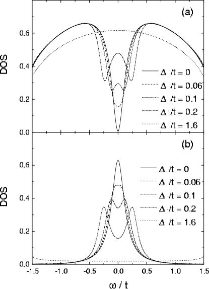
Figure 9: Local density of states for the side dot configuration corresponding to the symmetric situation $\varepsilon_{0}=-U/2$ for different magnetic fields: a) at the non-interacting site 0 of the tight-binding chain; b) at the QD site (same parameters as in Fig. 7).

V Conclusions

We have studied numerically the spin-dependent conductance of electrons through a single ballistic channel coupled to a side quantum dot. The Fano interference with the dot reverses the dependence of the channel conductance on the gate voltage compared to that of the substitutional dot’s conductance. If the spin degeneracy of the dot levels is lifted, the conductance of the channel reveals Coulomb blockade dips, or anti-resonances, as a function of the gate voltage. If the level is spin degenerate the Kondo effect suppresses the channel conductance in a broad range of the gate voltages.

When the coupling between the channel and the dot is not truly local the resonances should become highly antisymmetric. In the idealized picture of the single ballistic channel transport the zero temperature conductance vanishes at the resonance values of the gate voltage due to the Fano interference. If there is no spin degeneracy, the resonances have single-particle origin (for the simple model of Fig. 1b they are separated roughly by the Coulomb energy $U+\Delta$). At resonance the channel conductance for a certain spin direction changes abruptly from its ballistic value $e^{2}/h$ to zero, while the opposite spin conductance remains approximately at the ballistic value.

This is in contrast with previous calculations that considered a substitutional QD, where the complementary effect is found, i.e., a perfect conductance for one spin species. However, in these cases due to the local correlations and hibridization with the leads, there remains a finite conductance of the opposite spin species blurring the filtering condition. In the lateral dot case considered here we find total suppression of one spin species, thus leading to a perfect spin filter. Moreover we obtain that the energetical splitting of the Fano resonances for spin up and spin down electrons is of the order of the Coulomb interaction $U$ for large $U$ rather than of the order of the Zeeman splitting $\Delta$ as it would be for noninteracting electrons $U=0$. Thus a strong electron interaction on the dot (realistic values for $U$ are of the order of 1meV) will allow to apply very weak magnetic fields (less than 1Tesla) and still observe a significant splitting of the Fano resonances (provided $k_{B}T<\Delta$), and thus a high quality spin filter. This is because not only the spin filter is totally reflecting electrons with the desired spin $\sigma$, but it will be then also nearly fully transparent for electrons with opposite spin. Note, however, that the coupling to the dot should preserve the phase coherence and there should be only one conducting channel.

Figure 10: Local density of states at site 0 for up spins and the side dot configuration corresponding to: top: the symmetric situation $\varepsilon_{0}=-U/2$ and different magnetic fields; bottom: several gate voltage values $\varepsilon_{0}$ and small magnetic field $\Delta=0.1$.

We believe that our calculations also shed light on recent experiments by Göres et al.gores  Using the same samples of Ref.(david ), and changing the transmission of the left and right tunnel barriers which connect the dot to the conducting leads, they perform conductance measurements in the Fano regime (strong coupling leads-dot), the Kondo regime (intermediate coupling), and the Coulomb blockade regime (weak coupling leads-dot). The main results concern to the Fano regime, where the conductance shows asymmetric Fano dips on top of a slowly varying background. Some features of the dips are reminiscent of the Kondo effect, as the temperature dependence of the dips amplitudes (Fig. 4 in Ref. gores ), and others of the Coulomb blockade effect, as the typical diamond-shaped structure in differential conductance measurements (Fig. 5 in Ref. gores ). Both features are easily explained by our results. For example, from Fig. 8a, and considering that finite temperature weakens the Kondo resonance at the Fermi energy in a similar way as the magnetic field, one can expect a strong dependence of dip amplitude with temperature, with the dip amplitude decreasing for increasing temperature. Besides, the behavior of dips in differential conductance measurements should be completely analogous to the related Coulomb blockade peaks, leading to diamond-shaped structures for the dips. Our results also shed light on the somehow related problem of the persistent current in a mesoscopic ring with a side dot.affleck ; eckle The results remain controversial on this issue, as Ref. affleck found a detrimental effect of the side dot on the persistent current when the Kondo effect is operative. An opposite result was found in Ref. eckle , with the ring exhibiting a perfect (unitary) persistent current in the Kondo regime. Our results for the open configuration of the present work provide naturally strong support to the enhancement effect found by Affleck and Simon.affleck

The authors acknowledge CONICET for support. We would like to thank J. Simonin, M. Titov, S. Flach and A. Miroshnichenko for useful comments and discussions. Part of this work was done under projects Fundación Antorchas 14116-168 and 14116-212.

References

- (1) Mesoscopic Phenomena in Solids, B. L. Altshuler, P. A. Lee, and R. A. Web, editors, (North Holland, Amsterdam, 1991).
- (2) Mesoscopic Quantum Physics, E. Akkermans, G. Montambaux, J. L. Pichard, and J. Zinn-Justin, editors, (North Holland, Amsterdam, 1995).
- (3) Mesoscopic Electron Transport, L. L. Sohn, L. P. Kouwenhoven, and G. Schön, editors, (Kluwer, Dordreht, 1997).
- (4) Y. Alhassid, Rev. Mod. Phys. 72, 895 (2000).
- (5) I. L. Aleiner, P. W. Brouwer, and L. I. Glazman, Physics Reports 358, 309 (2002).
- (6) D. Goldhaber-Gordon, H. Shtrikman, D. Mahalu, D. Abush-Madger, U. Meirav, M. A. Kastner, Nature, 391, 156 (1998).
- (7) S. M. Cronenwet, T. H. Oosterkamp, and L. P. Kouwenhoven, Science 281, 540 (1998).
- (8) J. Schmid, J. Weis, K. Eberl, and K. von Klitzing, Physica B 256, 182 (1998).
- (9) J. Kondo, in Solid State Physics 23, 183 (1969).
- (10) A. C. Hewson, in The Kondo Problem to Heavy Fermions (Cambridge University Press, Cambridge, England, 1993).
- (11) L. I. Glazman and M. E. Raikh, JETP Lett. 47, 452 (1988).
- (12) T. K. Ng and P. A. Lee, Phys. Rev. Lett. 61, 1768 (1988).
- (13) It is interesting to note that only recently this unitary limit has been experimentally achieved: W. G. van der Wiel, S. De Franceschi, T. Fujisawa, J. M. Elzerman, S. Tarucha, and L. P. Kouwenhoven, Science 289, 2105 (2000).
- (14) L. P. Kouwenhoven, C. M. Marcus, P. L. McEuen, S. Tarusha, R. M. Westerweld, and N. S. Wingreen, in Ref. mesoscopic1 .
- (15) D. V. Averin and K. K. Likharev in Ref. mesoscopic3 .
- (16) V. Madhavan, W. Chen, T. Jamneala, M. F. Crommie, and N. S. Wingreen, Science 280, 567 (1998); J. Li, W-D Schneider, R. Berndt, and B. Delley, Phys. Rev. Lett. 80, 2893 (1998).
- (17) K. Kobayashi, H. Aikawa, A. Sano, S. Katsumoto and Y. Iye, preprint, cond-mat/0311497.
- (18) K. Kang, Y. Cho, Ju-Jin Kim, and Sung-Chul Shin, Phys. Rev. B 63, 113304 (2001).
- (19) A. Aligia and C. Proetto, Phys. Rev. B 65, 165305 (2002); P. Stefański, S. S. Comm. 128, 29 (2003)
- (20) R. Franco, M. S. Figueira and E. Anda, Phys. Rev. B 67, 155301 (2003).
- (21) J. Göres, D. Goldhaber-Gordon, S. Heemeyer, M. A. Kastner, H. Shtrikman, D. Mahalu, and U. Meirav, Phys. Rev. B 62, 2188 (2000).
- (22) T. Costi, Phys. Rev. B 64, 241310(R) (2001).
- (23) P. Recher, E. Sukhorukov and D. Loss, Phys. Rev. Lett. 85, 1962 (2000).
- (24) Y. Ohno, D. K. Young, B. Beschoten, F. Matsukura, H. Ohno, D. D. Awschalom, Nature 402, 790 (1999).
- (25) M. Popp, D. Frustaglia and K. Richter, preprint, cond-mat/0301064 (2003).
- (26) A. Kiselev and K. W. Kim, App. Phys. Lett. 78, 775 (2001).
- (27) D. Schmeltzer, A. Bishop. A. Saxena and D. Smith, Phys. Rev. Lett. 90, 116802 (2003).
- (28) M. E. Torio, K. Hallberg, A. H. Ceccatto, and C. R. Proetto, Phys. Rev. B 65, 085302 (2002).
- (29) M. E. Torio, K. Hallberg, S. Flach, A. E. Miroshnichenko, and M. Titov, Europhysics Journal (accepted for publication).
- (30) P. W. Anderson, Phys. Rev. 124, 41 (1961).
- (31) Y. Meir, N. S. Wingreen and P. A. Lee, Phys. Rev. Lett. 70, 2601 (1993).
- (32) P. Schlottmann, Phys. Rev. B 17, 2497 (1978).
- (33) Y. Meir and N. S. Wingreen, Phys. Rev. Lett. 68, 2512 (1992).
- (34) E. Dagotto and A. Moreo, Phys. Rev. D 31, 865 (1985); E. Gagliano, E. Dagotto, A. Moreo and F. Alcaraz, Phys. Rev. B 34, 1677 (1986).
- (35) V. Ferrari, G. Chiappe, E. V.Anda, and M. A. Davidovich, Phys. Rev. Lett. 82, 5088 (1999).
- (36) C. Caroli, R. Combescot, P. Nozieres and D. Saint-James , J. Phys. C 4, 916 (1971); W. Metzner, Phys. Rev. B 43, 8549 (1991).
- (37) D. S. Fisher and P. A. Lee, Phys. Rev. B 23, 6851 (1981).
- (38) D. C. Langreth, Phys. Rev. 150, 516 (1966).
- (39) P. B. Wiegmann and A. M. Tsvelick, J. Phys. C 16, 2281 (1983).
- (40) For a detailed derivation in the absence of magnetic fields we refer to Ref. kang .
- (41) B. R. Bulka and P. Stefanski, Phys. Rev. Lett., 86, 5128 (2001).
- (42) U. Fano, Phys. Rev., 124, 1866 (1961); J. A. Simpson and U. Fano, Phys. Rev. Lett., 11, 158 (1963).
- (43) I. Affleck and P. Simon, Phys. Rev. Lett. 86, 2854 (2001).
- (44) H.-P. Eckle, H. Johannesson, and C. A. Sttaford, Phys. Rev. Lett. 87, 016602 (2001).