Evolution of scale-free random graphs: Potts model formulation

Abstract

We study the bond percolation problem in random graphs of $N$ weighted vertices, where each vertex $i$ has a prescribed weight $P_{i}$ and an edge can connect vertices $i$ and $j$ with rate $P_{i}P_{j}$. The problem is solved by the $q\to 1$ limit of the $q$-state Potts model with inhomogeneous interactions for all pairs of spins. We apply this approach to the static model having $P_{i}\propto i^{-\mu}(0<\mu<1)$ so that the resulting graph is scale-free with the degree exponent $\lambda=1+1/\mu$. The number of loops as well as the giant cluster size and the mean cluster size are obtained in the thermodynamic limit as a function of the edge density, and their associated critical exponents are also obtained. Finite-size scaling behaviors are derived using the largest cluster size in the critical regime, which is calculated from the cluster size distribution, and checked against numerical simulation results. We find that the process of forming the giant cluster is qualitatively different between the cases of $\lambda>3$ and $2<\lambda<3$. While for the former, the giant cluster forms abruptly at the percolation transition, for the latter, however, the formation of the giant cluster is gradual and the mean cluster size for finite $N$ shows double peaks.

,

1 Introduction

In the last few years graph theoretic approach has been of great value to characterize complex systems found in social, informational and biological areas. Here, a complex system is represented as a graph or network whose vertices and edges stand for its constituents and interactions. A simplest model for such is the random graph model proposed by Erdős and Rényi (ER) [1]. In the ER model, $N$ number of vertices are present from the beginning and edges are added one by one in the system, connecting pairs of vertices selected randomly. Due to the randomness, the distribution of the number of edges incident on each vertex, called the degree distribution, is Poissonian. However, many real-world networks such as the World-wide web, the Internet, the coauthorship, the protein interaction networks and so on display power-law behaviors in the degree distribution. Such networks are called scale-free (SF) networks [2]. Thanks to recent extensive studies of SF networks, various properties of SF network structures have been uncovered [3, 4, 5].

There have been a few attempts to describe scale-free networks in the framework of equilibrium statistical physics, even though the number of vertices grows with time in many real-world networks [6, 7, 8, 9, 10]. In this approach, various mathematical tools developed in equilibrium statistical physics may be used to understand network structures. To proceed, one needs to define equilibrium network ensembles with appropriate weights, where one graph corresponds to one state of the ensemble. In a canonical ensemble, the number of edges $L$ is fixed: Given a degree distribution, $p_{d}(k)$, the mean degree $\langle k\rangle\equiv\sum kp_{d}(k)$ is obtained. Then the number of edges obtained through the relation, $L=\langle k\rangle N/2$, can be fixed. A degree sequence specifies the number of vertices with degree $k$ as $p_{d}(k)N$ [11, 12].

A grandcanonical ensemble can be also defined, where the number of edges is also a fluctuating variable while keeping the SF nature of the degree distributions. The grandcanonical ensemble for SF random graphs is realized in the static model introduced by Goh et al. [13] or in its generalized version investigated in Refs. [14]. The name ‘static’ originates from the fact that the number of vertices is fixed from the beginning. Here each vertex $i$ has a prescribed weight $P_{i}$ summed to 1 and an edge can connect vertices $i$ and $j$ with rate $P_{i}P_{j}$ [15, 16, 17]. A chemical potential-like parameter $K$ that can be regarded as “time” in the process of attaching edges controls the mean number of edges so that $\langle L\rangle$ increases with increasing $K$.

As the parameter $K$ increases, a giant cluster, or giant component, forms in the system. Here the giant cluster means the largest cluster of connected vertices whose size is ${\mathcal{O}}(N)$. Often such a giant cluster appears at the percolation transition point. In equilibrium statistical physics, the percolation problem can be studied through a spin model, the $q$-state Potts model in the $q\to 1$-limit [18]. Using the relation, in this paper, we study the evolution of SF random graphs from the perspective of equilibrium statistical physics. To be specific, we construct the $q$-state Potts model, where the interaction strength between each pair of vertices is inhomogeneous on the complete graph. In this formulation, since the interaction strength $K$ is tunable, the mean number of edges $\langle L\rangle$ varies. Thus, the grandcanonical ensemble is taken in the network representation. However, since the number of spins (vertices) is fixed, the formulation corresponds to a canonical ensemble in the spin-model representation. Note that our model is different from the one studied by Dorogovtsev et al., [19] where the Potts model is defined as a given fixed network so that each edge represents homogeneous interactions.

The formulation of the spin model facilitates explicit derivation of various properties of the SF network. Thus we derive the formula for the giant cluster size, the mean cluster size, and in particular, the number of loops and clusters. These quantities are explicitly evaluated analytically for the static model with $P_{i}\propto i^{-\mu}$, $(0<\mu<1)$ in the thermodynamic limit as a function of the edge density, and their critical properties are also studied. The degree exponent $\lambda$ is related to $\mu$ by $\lambda=1+1/\mu$. Moreover, their finite-size scaling behaviors are obtained using the finite largest cluster size for finite $N$ that in turn is evaluated from the cluster size distribution. From these, we are able to elucidate the process of formation of the giant cluster. While for the case $\lambda>3$, the giant cluster forms abruptly at the percolation transition point $K_{c}$, for the case $2<\lambda<3$ where most real world networks belong to, however, the formation of the giant cluster is gradual and the mean cluster size for finite $N$ show double peaks.

In fact, the percolation problem of SF networks has been studied, but in a different way, that is, by removing vertices one by one as well as their attached edges from an existing SF network [20, 21, 22]. The percolation transition was understood by using the branching process approach, which is supposed to be valid near the percolation transition point, where the network is sparse. In this paper, we provide the criterion for the validity of the branching process approach for a general degree distribution, and show that the branching process and the Potts model approaches are equivalent for the static model. Finally, note that while the branching process approach cannot count the number of loops, the Potts model formalism we use here enables us to count it.

This paper is organized as follows. We introduce in Sec. 2 an ensemble of random graphs where each vertex is weighted, and present in Sec. 3 the Potts model formulation to derive graph theoretical quantities from its free energy. In Sec. 4, the connection between the Potts model formulation and the branching process approach is discussed. The general results of Sec. 3 are applied to the static model in Sec. 5 to obtain explicitly the giant cluster size, the mean cluster size and the mean number of loops and clusters as a function of $K$. The cluster size distribution and the largest cluster size in finite size systems are obtained in Sec. 6. The finite-size scaling is presented and compared with numerical simulation results in Sec. 7. Finally Sec. 8 contains summary and discussion.

2 Random graphs with weighted vertices

Suppose that the number of vertices $N$ is fixed (static) and each vertex $i=1,\ldots,N$ is given a probability $P_{i}$ summed to 1. The ER model of random graphs corresponds to assigning $P_{i}=1/N$ for all $i$. To construct a SF graph, we use $P_{i}\sim i^{-\mu}$ with $0<\mu<1$. However, for the time being, $P_{i}$ is arbitrary as long as $P_{i}\ll 1$ for all $i$.

In each unit time duration, two vertices $i$ and $j$ are selected with probabilities $P_{i}$ and $P_{j}$. If $i=j$ or an edge connecting $i$ and $j$ already exists, do nothing; otherwise, an edge is added between the vertices $i$ and $j$. This process is repeated for $NK$ times. Then the probability that a given pair of vertices $i$ and $j$ ($i\neq j$) is not connected by an edge is given by $(1-2P_{i}P_{j})^{NK}\simeq e^{-2NKP_{i}P_{j}}$, while that it does is $1-e^{-2NKP_{i}P_{j}}$. Here we used the condition $P_{i}\ll 1$. The factor $2$ comes from the equivalence of $(ij)$ and $(ji)$. We use the “interaction” parameter $K$ for later convenience which controls the edge density $\langle L\rangle/N$. Since each edge $b_{ij}$ is produced independently, this process generates a graph $G$ with probability

$$P(G) = \prod_{b_{ij}\in G}(1-e^{-2NKP_{i}P_{j}})\prod_{b_{ij}\notin G}e^{-2NKP_{i}P_{j}}$$ (1)

$$= e^{-2NK\sum_{i>j}P_{i}P_{j}}\prod_{b_{ij}\in G}(e^{2NKP_{i}P_{j}}-1)$$

$$= e^{-NK(1-M_{2})}\prod_{b_{ij}\in G}(e^{2NKP_{i}P_{j}}-1),$$

where we used the notation $M_{n}\equiv\sum_{i=1}^{N}P_{i}^{n}$. By a graph $G$, we mean a configuration of undirected edges connecting a subset of $N(N-1)/2$ pairs of labelled vertices $i=1,2,\ldots,N$.

We then evaluate the ensemble average of any graph theoretical quantity $A$ by

$$\langle A\rangle=\sum_{G}P(G)A(G).$$ (2)

One example is the degree $k_{i}$ of a vertex $i$, the number of edges incident on $i$. To do this, the generating function of $k_{i}$, $g_{i}(\omega)\equiv\langle\omega^{k_{i}}\rangle$, is first calculated as

$$g_{i}(\omega)=\prod_{j(\neq i)}\left[e^{-2NKP_{i}P_{j}}+\omega(1-e^{-2NKP_{i}P_{j}})\right].$$ (3)

From this, one has

$$\langle k_{i}\rangle=\left.\omega{d\over d\omega}g_{i}(\omega)\right|_{\omega=1}=\sum_{j(\neq i)}(1-e^{-2NKP_{i}P_{j}}),$$ (4)

and the average degree $\langle k\rangle$ is

$$\langle k\rangle={2\langle L\rangle\over N}={1\over N}\sum_{i}\langle k_{i}\rangle={1\over N}\sum_{i\neq j}(1-e^{-2NKP_{i}P_{j}}).$$ (5)

Also,

$$\langle k_{i}^{2}\rangle = \left.\left(\omega{d\over d\omega}\right)^{2}g_{i}(\omega)\right|_{\omega=1}$$ (6)

$$= \left[\sum_{j(\neq i)}(1-e^{-2NKP_{i}P_{j}})\right]^{2}+\sum_{j(\neq i)}e^{-2NKP_{i}P_{j}}(1-e^{-2NKP_{i}P_{j}})$$

$$= \langle k_{i}\rangle+\langle k_{i}\rangle^{2}-\sum_{j(\neq i)}(1-e^{-2NKP_{i}P_{j}})^{2}.$$

We remark that Eq. (3) is rewritten as

$$g_{i}(\omega)\simeq e^{-(1-\omega)\langle k_{i}\rangle}$$ (7)

with $\langle k_{i}\rangle$ in Eq. (4) when $|(1-\omega)(1-e^{-2NKP_{i}P_{j}})|\ll 1$ for all $j(\neq i)$. It implies that the probability that $k_{i}$ is equal to $k$, $p_{d,i}(k)=\langle\delta_{k_{i},k}\rangle$, is given by

$$p_{d,i}(k)=\left.{1\over k!}{d^{k}\over d\omega^{k}}g_{i}(\omega)\right|_{\omega=0}\simeq{\langle k_{i}\rangle^{k}\over k!}e^{-\langle k_{i}\rangle}$$ (8)

for $k\gg 1$. Other quantities are discussed later on.

3 Potts model

3.1 Potts model and random graph

It is well known that the $q$-state Potts model provides a useful connection between the geometric bond percolation problem and the thermal systems through the Kasteleyn construction [18]. The $q\to 1$ limit of the Potts model corresponds to the bond percolation problem. The same approach can be used for the random graph problem. From the viewpoint of the thermal spin system, this is basically the infinite range model since all pairs of spins interact with each other albeit with inhomogeneous interaction strength.

Consider the $q$-state Potts Hamiltonian given by

$$-H=2NK\sum_{i>j}P_{i}P_{j}\delta(\sigma_{i},\sigma_{j})+h_{0}\sum_{i=1}^{N}[q\delta(\sigma_{i},1)-1],$$ (9)

where $K$ is the interaction, $h_{0}$ is a symmetry-breaking field, $\delta(x,y)$ the Kronecker delta function, and $\sigma_{i}$ the Potts spins taking integer values $1,2,\ldots,q\equiv r+1$. We use the notation $r\equiv q-1$. The partition function $Z_{N}(q,h_{0})$ can be written as

$$Z_{N}(q,h_{0}) = {\rm Tr}\,e^{-H}={\rm Tr}\,\prod_{i>j}\left[1+(e^{2NKP_{i}P_{j}}-1)\delta(\sigma_{i},\sigma_{j})\right]$$ (10)

$$\times\prod_{i}e^{h_{0}(q\delta(\sigma_{i},1)-1)},$$

where Tr denotes the sum over $q^{N}$ spin states. Expanding the first product and taking the Tr operation, one has

$$Z_{N}(q,h_{0})=\sum_{G}\prod_{b_{ij}\in G}(e^{2NKP_{i}P_{j}}-1)\prod_{s\geq 1}(e^{srh_{0}}+re^{-sh_{0}})^{n_{G}(s)},$$ (11)

where $n_{G}(s)$ is the number of $s$-clusters, a cluster with $s$ vertices in a given graph $G$. Comparing this with Eq. (1), one immediately notices that

$$Z_{N}(q,h_{0})=e^{NK(1-M_{2})}\sum_{G}P(G)\prod_{s\geq 1}(e^{srh_{0}}+re^{-sh_{0}})^{n_{G}(s)}.$$ (12)

In particular, $Z_{N}(q,0)=e^{NK(1-M_{2})}\langle q^{C}\rangle$, where $C=\sum_{s}n_{G}(s)$ is the total number of clusters in graph $G$. Thus $Z_{N}(q,0)$ is the generating function of $C$.

The magnetization of the Potts model is defined as

$$m(q,h_{0})={1\over rN}{\partial\over\partial h_{0}}\ln Z_{N}(q,h_{0}).$$ (13)

It can be written as

$$m(q,h_{0})={\left\langle\sum_{\rm clusters}\left[{e^{srh_{0}}-e^{-sh_{0}}\over e^{srh_{0}}+re^{-sh_{0}}}\right]\left({s\over N}\right)\prod_{\rm clusters}(e^{srh_{0}}+re^{-sh_{0}})\right\rangle\over\langle\prod_{\rm clusters}(e^{srh_{0}}+re^{-sh_{0}})\rangle}.$$ (14)

If we introduce the cluster size distribution $P(s)\equiv n(s)(s/N)$ with $n(s)=\langle n_{G}(s)\rangle$ and the generating function $\mathcal{P}(z)=\sum_{s\geq 1}P(s)z^{s}$, the magnetization is, when $q=1$,

$$m(1,h_{0})=\sum_{s\geq 1}P(s)\left(1-e^{-sh_{0}}\right)=1-\mathcal{P}(e^{-h_{0}}).$$ (15)

The generating function $\mathcal{P}(z)$ will be used in Sec. 6 to investigate the asymptotic behavior of the cluster size distribution.

When $h_{0}=0$, the magnetization vanishes for finite $N$. However, when we take the limit $h_{0}\to 0$ after the thermodynamic limit $N\to\infty$, the contribution from the largest cluster whose size is $S$ can survive to give

$$m(1,h_{0}\to 0)=\left\langle{S\over N}\right\rangle,$$ (16)

if $S/N$ is finite. Let us define a giant cluster by a cluster whose size is $\mathcal{O}(N)$. Then $m(1,h_{0}\to 0)$ is the ratio of the giant cluster size to $N$, if it exists, and the system is considered as being in the percolating phase if $m(1,h_{0}\to 0)$ is non-zero. For simplicity, we will call $m(1,h_{0}\to 0)$ the giant cluster size and denote it by $m$.

The susceptibility defined as $\chi(q,h_{0})\equiv(1/q)(\partial/\partial h_{0})m(q,h_{0})$ on the other hand is related to the mean cluster size:

$$\chi(1,h_{0}\to 0)=\lim_{h_{0}\to 0}\lim_{N\to\infty}\sum_{s}P(s)se^{-sh_{0}}=\sum_{s\neq\langle S\rangle}sP(s),$$ (17)

where $h_{0}\langle S\rangle\to\infty$ is used with $\langle S\rangle$ the ensemble average of the largest cluster size, which we call simply the largest cluster size. We will denote $\chi(1,h_{0}\to 0)$ by $\bar{s}$. Note that our definition of $\bar{s}$ is normalized with respect to the total number of vertices instead of the number of vertices belonging to finite clusters.

The number of loops $N_{\rm loop}$ is related to the total number of clusters $C$ through

$$N_{\rm loop}=L-N+C.$$ (18)

Since $Z_{N}(q,0)\sim\langle q^{C}\rangle$, one can notice that the number of loops per vertex $\langle N_{\rm loop}\rangle/N$ is given as

$${\langle N_{\rm loop}\rangle\over N}={\langle L\rangle\over N}-1+{1\over N}{\partial\over\partial q}\left[\ln Z_{N}(q,0)\right]_{q=1}.$$ (19)

We will denote $\langle N_{\rm loop}\rangle/N$ by $\ell$ and call it the number of loops for simplicity.

Figure 1: Vector representations of $q$-state Potts spins with $q=2$, $3$, and $4$.

3.2 Partition function

A convenient way to evaluate the partition function is to resort to the vector-spin representation where one associates an $r$-dimensional vector $\vec{S}(\sigma_{i})$ of unit length to each spin value $\sigma_{i}$, where $\vec{S}(1)=(1,0,\ldots,0)$ and $\vec{S}(\sigma_{i})$ with $\sigma_{i}=2,3,\ldots,q$ point to the remaining $r$ corners of the $r$-dimensional tetrahedron (See Fig. 1). Then one can represent the Kronecker delta function as a dot product between $\vec{S}$’s,

$$\delta(\sigma_{i},\sigma_{j})={1\over q}(r\,\vec{S}(\sigma_{i})\cdot\vec{S}(\sigma_{j})+1).$$ (20)

Using this, the interaction term in Eq. (9) can be written as

$$2NK\sum_{i>j}P_{i}P_{j}\delta(\sigma_{i},\sigma_{j})=NK\left({1\over q}-M_{2}\right)+{rNK\over q}\left(\sum_{i}P_{i}\vec{S}(\sigma_{i})\right)^{2}.$$ (21)

The perfect square is then linearized through the identity $\int dye^{-ay^{2}+by}=\sqrt{\pi/a}\,e^{b^{2}/(4a)}$. Thus we have

$$Z_{N}(q,h_{0})={\rm Tr}\,\left[e^{NK(\frac{1}{q}-M_{2})}\left({4\pi K\over rqN}\right)^{-\frac{r}{2}}e^{\sum_{i=1}^{N}r\vec{h_{0}}\cdot\vec{S}(\sigma_{i})}\int d\vec{y}\,e^{-{rqN\over 4K}y^{2}+rN\sum_{i=1}^{N}P_{i}\vec{y}\cdot\vec{S}(\sigma_{i})}\right],$$ (22)

where the integration is over the $r$-dimensional space and $\vec{h_{0}}=(h_{0},0,\ldots,0)$. Now the Tr operation can be performed for each spin independently. Defining

$$\tilde{\zeta}(\vec{h})={1\over q}\sum_{\sigma=1}^{q}e^{r\vec{h}\cdot\vec{S}(\sigma)},$$ (23)

one then has

$$Z_{N}(q,h_{0})=\left({4\pi K\over rqN}\right)^{-\frac{r}{2}}q^{N}e^{NK(\frac{1}{q}-M_{2})}\int d\vec{y}\,e^{-{rqN\over 4K}y^{2}+\sum_{i=1}^{N}\ln\tilde{\zeta}(\vec{h_{0}}+NP_{i}\vec{y})}.$$ (24)

Provided $(1/N)\sum_{i=1}^{N}\ln\tilde{\zeta}(\vec{h_{0}}+NP_{i}\vec{y})$ has a well-defined limit as $N\to\infty$, one can apply the saddle point method to Eq. (24), where the integral is replaced by the value of the integrand at its maximum. The maximum is for $\vec{y}$ which is a solution of the saddle-point equation

$${q\over 2K}\vec{y}={1\over rN}\sum_{i=1}^{N}\nabla_{\vec{y}}\ln\tilde{\zeta}(\vec{h_{0}}+NP_{i}\vec{y}).$$ (25)

When $\vec{h}_{0}=0$, $\vec{y}=0$ is always a solution of Eq. (25), but the spontaneous symmetry-breaking solutions ($\vec{y}\neq 0$) with the Potts symmetry may appear for large $K$. When the symmetry-breaking field is applied along the $1$-direction, $\vec{h}_{0}=(h_{0},0,\ldots,0)$, the nontrivial physically relevant solution of Eq. (25) is expected in the sub-manifold $\vec{y}=(y,0,\ldots,0)$. The limit $h_{0}\rightarrow 0^{+}$ then selects one of the $q$ equivalent spontaneous symmetry-breaking solutions. With this in mind, we may restrict our attention to the one-dimensional sub-manifold of $\vec{y}$ in Eqs. (24) and (25). As a result, we then have, as $N\to\infty$,

$${1\over N}\ln Z_{N}(q,h_{0})=\ln q+K\left({1\over q}-M_{2}\right)-rF(y,h_{0}),$$ (26)

with

$$F(y,h_{0})={q\over 4K}y^{2}-{1\over rN}\sum_{i=1}^{N}\ln\zeta(h_{0}+NP_{i}y,q),$$ (27)

where

$$\zeta(h,q)={1\over q}\sum_{\sigma=1}^{q}e^{rS_{1}(\sigma)}={e^{rh}+re^{-h}\over 1+r},$$ (28)

and $y$ is the solution of the one-dimensional saddle-point equation,

$${q\over 2K}y={1\over r}\sum_{i=1}^{N}P_{i}{\partial\over\partial h_{0}}\ln\zeta(h_{0}+NP_{i}y,q).$$ (29)

Here, the $q$-dependence in $F(y,h_{0})$ is not shown explicitly. Since $m=(1/(rN))(\partial/\partial h_{0})\ln Z$, we see that

$$m(q,h_{0})=-{d\over dh_{0}}F(y,h_{0})={1\over rN}\sum_{i=1}^{N}{\partial\over\partial h_{0}}\ln\zeta(h_{0}+NP_{i}y,q).$$ (30)

At this point, it is useful to take the $r\to 0$ limit in Eqs. (27), (29), and (30), which yields, with $h_{i}=h_{0}+NP_{i}y$,

$$F(y,h_{0})={1\over 4K}y^{2}-{1\over N}\sum_{i=1}^{N}(e^{-h_{i}}-1+h_{i}),$$ (31)

where $y$ is the solution of

$${y\over 2K}=\sum_{i=1}^{N}P_{i}(1-e^{-h_{i}}).$$ (32)

The magnetization and the susceptibility reduce to

$$m(1,h_{0})={1\over N}\sum_{i=1}^{N}(1-e^{-h_{i}}),$$ (33)

and

$$\chi(1,h_{0}) = {1\over N}\sum_{i=1}^{N}e^{-h_{i}}(1+NP_{i}{dy\over dh_{0}}),$$ (34)

$$= {1\over N}\sum_{i=1}^{N}e^{-h_{i}}+{\left(\sum_{i=1}^{N}P_{i}e^{-h_{i}}\right)^{2}\over(2K)^{-1}-\sum_{i=1}^{N}NP_{i}^{2}e^{-h_{i}}},$$

respectively, where it is used that

$${dy\over dh_{0}}={\sum_{i=1}^{N}P_{i}e^{-h_{i}}\over(2K)^{-1}-\sum_{i=1}^{N}NP_{i}^{2}e^{-h_{i}}}.$$ (35)

Thus the giant cluster size and the mean cluster size are obtained from Eqs. (33) and (34), respectively, with $h_{0}\to 0$.

Also, the number of clusters per vertex is

$${\langle C\rangle\over N}=1-K-F(y,0)|_{q=1},$$ (36)

while that of loops is

$${\langle N_{\rm loop}\rangle\over N}={\langle L\rangle\over N}-K-F(y,0)|_{q=1},$$ (37)

where $y$ is given by Eq. (32) with $h_{0}=0$.

When $h_{0}\to 0$, a non-trivial solution of Eq. (32) begins to appear when $(2K)^{-1}<N\sum_{i=1}^{N}P_{i}^{2}$, which gives the following characteristic value $K_{c}$

$$K_{c}={1\over 2N\sum_{i=1}^{N}P_{i}^{2}}.$$ (38)

When $P_{i}$ decays slower than $i^{-1}$ and $KP_{i}\ll 1$ for all $i$, $\langle k\rangle=2K$ and $\langle k^{2}\rangle=(1/N)\sum_{i=1}^{N}\langle k_{i}^{2}\rangle=\langle k\rangle+N^{-1}\sum_{i=1}^{N}\langle k_{i}\rangle^{2}=2K+4NK^{2}\sum_{i=1}^{N}P_{i}^{2}$, which will be shown below. Then the condition $K=K_{c}$ is equivalent to the well-known condition $\langle k^{2}\rangle/\langle k\rangle=2$ [11]. Whether the percolation transition occurs at $K_{c}$ or not will be investigated for specific $P_{i}$’s of the static model.

4 Branching process approach

The cluster size distribution $P(s)$ can be obtained from Eqs. (32) and (33) using $m(1,h_{0})=1-\mathcal{P}(e^{-h_{0}})$ and $P(s)=(1/s!)d^{s}\mathcal{P}(z)/dz^{s}|_{z=0}$. However, the cluster size distribution can also be obtained through the generating function approach or equivalently the branching process approach. Here, the presence of loops in finite clusters is neglected and each cluster in a given graph is considered as a tree generated by successive branchings from an arbitrary vertex  [23, 24]. Consider the probability that a randomly chosen vertex belongs to a $s$-cluster, which is just $P(s)$. Then $P(s)$ can be written recursively as

$$P(s)=\delta_{s,1}p_{d}(0)+\sum_{k\geq 1}p_{d}(k)\prod_{i=1}^{k}\sum_{s_{i}}R(s_{i})\,\delta_{\sum_{i}s_{i},s-1},$$ (39)

where $p_{d}(k)$ is the degree distribution and $R(s)$ is the probability that a randomly-chosen edge has a $s$-cluster at its one end, and thus equal to the number of edges followed by $s$-clusters divided by $2L$. $R(s)$ is obtained self-consistently as

$$R(s)=\delta_{s,1}r_{d}(0)+\sum_{k\geq 1}r_{d}(k)\prod_{i=1}^{k}\sum_{s_{i}}R(s_{i})\,\delta_{\sum_{i}s_{i},s-1},$$ (40)

where $r_{d}(k)$ is the probability that the vertex at either end of a randomly-chosen edge has $k+1$ edges and thus is equal to $(k+1)p_{d}(k+1)/\langle k\rangle$. With the generating functions $\mathcal{P}(z)=\sum_{s=1}^{\infty}P(s)z^{s}$ and $\mathcal{R}(z)=\sum_{s=1}^{\infty}R(s)z^{s}$, Eqs. (39) and (40) can be written in more compact forms as

$$\mathcal{P}(z)=zg(\mathcal{R}(z))$$ (41)

and

$$\mathcal{R}(z)=zf(\mathcal{R}(z)),$$ (42)

where $g(\omega)=\sum_{k=0}^{\infty}p_{d}(k)\omega^{k}$ and $f(\omega)=g^{\prime}(\omega)/\langle k\rangle=g^{\prime}(\omega)/g^{\prime}(1)$. We mention that Eqs. (41) and (42) with $z=1$ are equivalent to those derived by Molloy and Reed [11] for a given degree sequence.

Eqs. (41) and (42) are the standard results. For the grandcanonical ensemble we are using, the generating functions $g(\omega)$ and $f(\omega)$ are represented in terms of $g_{i}(\omega)$, the generating function of $p_{d,i}(k)$ in Eq. (3), as

$$g(\omega) = {1\over N}\sum_{i=1}^{N}g_{i}(\omega)$$

$$f(\omega) = {1\over N\langle k\rangle}\sum_{i=1}^{N}{dg_{i}(\omega)\over d\omega}$$ (43)

with $\langle k\rangle=g^{\prime}(1)$. In particular, if

$$g_{i}(\omega)=e^{-(1-\omega)2NKP_{i}},$$ (44)

which holds, for example, when $1-e^{-2NKP_{i}P_{j}}\ll 1$ for all $i\neq j$, then Eqs. (41) and (42) of the branching process approach are exactly equal to Eqs. (33) and (32) of the Potts model formulation, identifying $z$, $\mathcal{P}(z)$, and $\mathcal{R}(z)$ with $e^{-h_{0}}$, $1-m(1,h_{0})$, and $1-y/(2K)$, respectively.

5 Percolation of the Static model: Thermodynamic limit

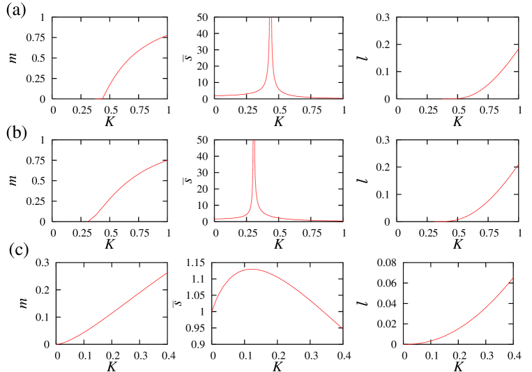
Figure 2: Giant cluster size $m$, mean cluster size $\bar{s}$, and number of loops $\ell=\langle N_{\rm loop}\rangle/N$ vs. $K$ for $\mu=5/19$ ($\lambda=4.8$) (a), $\mu=5/13$ ($\lambda=3.6$) (b), and $\mu=5/7$ ($\lambda=2.4$) (c). They are obtained by solving numerically Eqs. (51), (57), and (64), respectively, together with Eq. (52). The number of clusters per vertex not shown here is $1-K+\ell$ and monotonically decreases with $K$ from 1 to 0.

So far, our discussion applies to arbitrary $P_{i}$. In this section, we specialize to the case of the static model,

$$P_{i}={i^{-\mu}\over\zeta_{N}(\mu)}\quad(0<\mu<1).$$ (45)

Here $\zeta_{N}(x)\equiv\sum_{i=1}^{N}i^{-x}$, and in the limit $N\to\infty$, it converges to the Riemann zeta function $\zeta(x)$ when $x>1$ and diverges as $N^{1-x}/(1-x)$ when $0<x<1$. In the marginal case with $x=1$, it is calculated as $\ln N+\gamma_{M}$ with $\gamma_{M}=0.5772\ldots$, the Euler-Mascheroni constant. The sum appearing in Eq. (31) is evaluated in Appendix A as

$$\Sigma_{1}(y) \equiv {1\over N}\sum_{i=1}^{N}e^{-NP_{i}y}$$ (46)

$$= -\Gamma\left(1-{1\over\mu}\right)(1-\mu)^{1\over\mu}y^{1\over\mu}+1-y+{(1-\mu)^{2}\over 2(1-2\mu)}y^{2}+\cdots$$

for $y(1-\mu)N^{\mu}\gg 1$. This will be used repeatedly. We do not consider the marginal cases where $1/\mu$ is an integer. The sums in Eqs. (4) and (5) are evaluated using $\Sigma_{1}(y)$ to give

$$\langle k_{i}\rangle=2NKP_{i}\quad{\rm and}\quad\langle k\rangle=2\langle L\rangle/N=2K,$$ (47)

in the limit $N\to\infty$ if $KP_{i}\ll 1$ for all $i$ or equivalently, $K\ll\zeta_{N}(\mu)=\mathcal{O}(N^{1-\mu})$. Thus $K$ is $\langle L\rangle/N$. Under the same condition, the third term $(1-e^{-2NKP_{i}P_{j}})^{2}$ in Eq. (6) does not contribute to $\langle k^{2}\rangle=(1/N)\sum_{i=1}^{N}\langle k_{i}^{2}\rangle$ in the limit $N\to\infty$, which gives $\langle k^{2}\rangle=(1/N)\sum_{i=1}^{N}[\langle k_{i}\rangle+\langle k_{i}\rangle^{2}]$. Moreover, rewriting Eq. (3) as

$$\log g_{i}(\omega)=\sum_{j(\neq i)}\log\left[1-(1-\omega)(1-e^{-2NKP_{i}P_{j}})\right]$$ (48)

and expanding the right hand side as a power series in $(1-\omega)$ to apply the result of Appendix A, we find that Eq. (44) holds for all range of $0<\mu<1$ and $K$ finite. Note that $(1-e^{-2NKP_{i}P_{j}})$ is not small when $1/2<\mu<1$ but the final result is the same as that for $0<\mu<1/2$ where $(1-e^{-2NKP_{i}P_{j}})\simeq 2NKP_{i}P_{j}\ll 1$ holds. Thus the degree of each vertex $k_{i}$ follows the Poisson distribution and the branching process approach and the Potts model approach are equivalent for the static model as long as $m$ and ${\bar{s}}$ are concerned. This is because the finite clusters remain effectively trees for all $K$.

For convenience, we divide the range of $\mu$ into the three cases, (I) $0<\mu<1/3$, (II) $1/3<\mu<1/2$, and (III) $1/2<\mu<1$.

5.1 Degree distribution

The asymptotic behavior of the degree distribution $p_{d}(k)$ is related to the behavior of its generating function $g(\omega)=\sum_{k}p_{d}(k)\omega^{k}$ for $\omega$ near $1$, which is equal to $\Sigma_{1}(2K(1-\omega))$ in the limit $N\to\infty$. The latter condition is necessary for the approximation $P_{i}(1-P_{i})\simeq P_{i}$ to be valid. From Eqs. (115) and (119), the degree distribution $p_{d}(k)$ is given by

$$p_{d}(k)={1\over k!}\left.{d^{k}\over d\omega^{k}}g(\omega)\right|_{\omega=0}\simeq\left\{\begin{array}[]{ll}c_{1}k^{-1-\frac{1}{\mu}}&{\rm for}\ 1\ll k\ll k_{\rm max},\\[7.11317pt] c_{2}\frac{k_{\rm max}^{k}}{k!}&{\rm for}\ k\gg k_{\rm max},\end{array}\right.$$ (49)

where $k_{\rm max}$ is equal to $\langle k_{1}\rangle$ i.e., $k_{\rm max}=2K(1-\mu)N^{\mu}$, $c_{1}=(1/\mu)[2K(1-\mu)]^{1/\mu}$ and $c_{2}=(1/N)\sum_{r=0}^{\infty}(-k_{\rm max})^{r}\zeta[\mu(k+r)]/r!\simeq e^{-k_{\rm max}}/N$. From now on, we assume that $K_{\ell}\ll K\ll K_{u}$ with $K_{\ell}\equiv N^{-\mu}/(2(1-\mu))$ and $K_{u}\equiv N^{1-\mu}/(2(1-\mu))$, for which $1\ll k_{\rm max}\ll N$ so that there exists the regime of $k$ where the degree distribution follows a power law $p_{d}(k)\sim k^{-\lambda}$ with

$$\lambda=1+{1\over\mu}.$$ (50)

Since we are interested in the range $0<\mu<1$, the degree exponent $\lambda$ is larger than $2$.

5.2 Giant cluster size

The giant cluster size $m$ can be evaluated by Eq. (33) with $h_{i}=NP_{i}y$. In terms of $\Sigma_{1}(y)$ evaluated in Appendix A, it is simply represented as

$$m=1-\Sigma_{1}(y)$$ (51)

with $y$ obtained by solving Eq. (32)

$${y\over 2K}=\sum_{i=1}^{N}P_{i}(1-e^{-h_{i}})=1+\Sigma_{1}^{\prime}(y),$$ (52)

where $\Sigma_{1}^{\prime}(y)=(d/dy)\Sigma_{1}(y)$.

When $y$ is small, Eq. (52) is expanded as

$$({\rm I})~{}~{}~{}{y\over 2K} \simeq {y\over 2K_{c}}-{(1-\mu)^{3}\over 2(1-3\mu)}y^{2},$$

$$({\rm II})~{}~{}~{}{y\over 2K} \simeq {y\over 2K_{c}}-\Gamma\left(1-\frac{1}{\mu}\right){(1-\mu)^{1\over\mu}\over\mu}y^{\frac{1}{\mu}-1},$$

$$({\rm III})~{}~{}~{}{y\over 2K} \simeq -\Gamma\left(1-\frac{1}{\mu}\right){(1-\mu)^{1\over\mu}\over\mu}y^{\frac{1}{\mu}-1},$$ (53)

for the three ranges of $\mu$, (I), (II), and (III), respectively. For (I) and (II), the characteristic value $K_{c}$ defined by

$$K_{c}={(1-2\mu)\over 2(1-\mu)^{2}}$$ (54)

appears, which is just Eq. (38) with $P_{i}$ in Eq. (45).

When $K<K_{c}$ for (I) and (II), or $K=0$ for (III), Eqs. (52) or (53) has the solution $y=0$, and therefore, the giant cluster size is

$$m=0.$$ (55)

That is, there is no giant cluster for $K<K_{c}$ (I, II) or $K=0$ (III). But a non-zero solution for $y$ occurs when $K>K_{c}$ (I, II) or $K>0$ (III). It leads to the following giant cluster size $m$:

$$({\rm I})~{}~{}~{} m\simeq y\simeq{2(1-3\mu)\over(1-\mu)(1-2\mu)}\Delta,$$

$$({\rm II})~{}~{}~{} m\simeq y\simeq{1\over 1-\mu}\left({\mu\over(1-2\mu)\Gamma\left(1-\frac{1}{\mu}\right)}\right)^{\mu\over 1-2\mu}\Delta^{\mu\over 1-2\mu},$$

$$({\rm III})~{}~{}~{} m\simeq y\simeq\left({2(1-\mu)^{1\over\mu}\left|\Gamma\left(1-\frac{1}{\mu}\right)\right|\over\mu}\right)^{\mu\over 2\mu-1}K^{\mu\over 2\mu-1},$$ (56)

for $\Delta\equiv K/K_{c}-1$ (I, II) or $K$ (III) small and positive. Here the relation $m\simeq y$ comes from Eqs. (51) and (119). The giant cluster size is finite for $\Delta$ finite and positive, and thus $K_{c}$ is the percolation transition point. If we define a critical exponent $\beta$ by $m\sim\Delta^{\beta}$, its value is $1$ (I) and $\mu/(1-2\mu)$ (II). For (III), $m$ is finite for $K$ finite, but $K=0$ is not a percolation transition point, which will be investigated further below.

The giant cluster size $m$ as a function of $K$, which can be obtained numerically from Eqs. (51) and (52), is plotted for the case of $\mu=5/19$ ($\lambda=1+1/\mu=4.8$), $5/13$ ($\lambda=3.6$), and $5/7$ ($\lambda=2.4$) in Fig. 2.

We mention that in Ref. [16], some rigorous bounds of the giant cluster size are derived for an ensemble similar to ours, but with a different form of the probabilities of adding edges so that their results apply only to the case $\lambda>3$ of the static model.

5.3 Mean cluster size

The mean cluster size $\bar{s}$ or the susceptibility $\chi(1,h_{0}\to 0)$ in Eq. (34) is represented in terms of $\Sigma_{1}(y)$ in Appendix A as

$$\bar{s}=\Sigma_{1}(y)+{[\Sigma_{1}^{\prime}(y)]^{2}\over(2K)^{-1}-\Sigma_{1}^{\prime\prime}(y)},$$ (57)

where $y$ is the solution of Eq. (52) and $\Sigma_{1}^{\prime\prime}(y)=(d/dy)\Sigma_{1}^{\prime}(y)$.

When $K<K_{c}$ for (I) and (II), $y=0$ and thus

$$\bar{s}=1+{2KK_{c}\over K_{c}-K}$$ (58)

since $\Sigma(0)=-\Sigma^{\prime}(0)=1$, and $\Sigma_{1}^{\prime\prime}(y)=1/(2K_{c})$. On the other hand, when $K>K_{c}$, $y$ is non-zero but given by Eq. (56), and one can see that $\Sigma(y)\simeq 1$, $\Sigma^{\prime}(y)\simeq-1$ and

$$\Sigma^{\prime\prime}(y)\simeq\left\{\begin{array}[]{ll}\frac{1}{2K_{c}}-\frac{\Delta}{K_{c}}&{\rm(I)},\\ \frac{1}{2K_{c}}-\frac{1-\mu}{2\mu}\frac{\Delta}{K_{c}}&{\rm(II)}.\end{array}\right.$$ (59)

From these relations, the mean cluster size for $K$ around $K_{c}$ is obtained as

$$\bar{s}\simeq\left\{\begin{array}[]{ll}{c_{-}\over(-\Delta)}&(\Delta<0)\\ {c_{+}\over\Delta}&(\Delta>0)\end{array}\right.,$$ (60)

where

$$c_{-}=2K_{c},\quad c_{+}=\left\{\begin{array}[]{ll}2K_{c}&{\rm(I)},\\ {2\mu\over 1-2\mu}K_{c}&{\rm(II)}.\end{array}\right.$$ (61)

$\bar{s}$ diverges at $K_{c}$ both for (I) and (II). Thus, if we define $\chi\sim|\Delta|^{-\gamma}$, then $\gamma=1$ for both (I) and (II).

For (III), $y$, the solution of Eq. (52) is zero only when $K$ is zero. We suppose that $K$ is non-zero but small in the thermodynamic limit $N\to\infty$. Then, from Eq. (119), it follows that

$$\Sigma_{1}(y) \simeq 1-\left({2B\over\mu}\right)^{\mu\over 2\mu-1}K^{\mu\over 2\mu-1}+\left({2\over\mu}\right)^{1\over 2\mu-1}B^{2\mu\over 2\mu-1}K^{1\over 2\mu-1},$$

$$\Sigma_{1}^{\prime}(y) \simeq -1+{1\over 2}\left({2B\over\mu}\right)^{\mu\over 2\mu-1}K^{1-\mu\over 2\mu-1},$$

$$\Sigma_{1}^{\prime\prime}(y) \simeq \frac{1-\mu}{2\mu K},$$ (62)

where $B=(1-\mu)^{1/\mu}|\Gamma(1-1/\mu)|$. Then the mean cluster size is

$$\bar{s} \simeq 1-\left({2B\over\mu}\right)^{\mu\over 2\mu-1}K^{\mu\over 2\mu-1}+\left({2\over\mu}\right)^{1\over 2\mu-1}B^{2\mu\over 2\mu-1}K^{1\over 2\mu-1}+{2\mu K\over 2\mu-1}\left(1-{1\over 2}\left({2B\over\mu}\right)^{\mu\over 2\mu-1}K^{1-\mu\over 2\mu-1}\right)^{2}$$ (63)

$$\simeq 1+{2\mu\over 2\mu-1}K-{4\mu-1\over 2\mu-1}\left({2B\over\mu}\right)^{\mu\over 2\mu-1}K^{\mu\over 2\mu-1}+{\mu^{2}\over 2\mu-1}\left({2B\over\mu}\right)^{2\mu\over 2\mu-1}K^{1\over 2\mu-1},$$

for small $K$. As shown in the numerical solutions for the mean cluster size $\bar{s}$ obtained from Eqs. (57) and (52) plotted in Fig. 2, the most important feature of $\bar{s}$ for (III) is that it does not diverge at any value of $K$ but has only a finite peak at $K_{p2}=\mathcal{O}(1)$. It implies that there is no phase transition for (III), i.e., $2<\lambda<3$.

5.4 Number of loops and clusters

The number of loops per vertex $\langle N_{\rm loop}\rangle/N$, which we denote by $\ell$, is also represented in terms of $\Sigma_{1}(y)$ as

$$\ell=-F(y,0)=-1+y-{1\over 4K}y^{2}+\Sigma_{1}(y),$$ (64)

with $y$ being the solution of Eq. (52).

When $K<K_{c}$ for (I) and (II), and $K=0$ for (III), the value of $y$ is zero and $\Sigma_{1}(0)=1$, which leads to

$$\ell=0.$$ (65)

On the other hand, when $K>K_{c}$ for (I, II), or $K>0$ for (III), the value of $\ell$ is not zero. From the behavior of $\Sigma_{1}(y)$ for small $y$ and Eq. (56), one can see that for $\Delta>0$ (I, II) or $K>0$ (III),

$$\ell\simeq\left\{\begin{array}[]{ll}{2\over 3}{(1-3\mu)^{2}\over(1-2\mu)^{3}}\Delta^{3}&({\rm I}),\\[7.11317pt] {1\over 2}\left({\mu\over(1-2\mu)\Gamma\left(1-\frac{1}{\mu}\right)}\right)^{2\mu\over 1-2\mu}\Delta^{1\over 1-2\mu}&({\rm II}),\\[7.11317pt] {2\mu-1\over 4}\left({2(1-\mu)^{1\over\mu}\left|\Gamma\left(1-\frac{1}{\mu}\right)\right|\over\mu}\right)^{2\mu\over 2\mu-1}K^{1\over 2\mu-1}&({\rm III}).\end{array}\right.$$ (66)

The exact solutions for $\ell$ are shown in Fig. 2. The number of clusters is simply related to $\ell$ as $\langle C\rangle/N=1-K+\ell$.

6 Cluster size distribution and largest cluster size

Beyond the largest cluster size or the mean cluster size, the whole distribution of cluster size $P(s)$ for the static model can be derived from Eqs. (32) and (33), which gives the parametrized equations for $\mathcal{P}(z)=1-m(1,h_{0}=-\ln z)$ as

$$z={1-{y\over 2K}\over\sum_{i=1}^{N}P_{i}e^{-NP_{i}y}}=-{1-{y\over 2K}\over\Sigma_{1}^{\prime}(y)},$$

$$\mathcal{P}(z)={z\over N}\sum_{i=1}^{N}e^{-NP_{i}y}=z\Sigma_{1}(y),$$ (67)

where $\Sigma_{1}(y)$ in Appendix A is used. $P(s)$ is obtained by $P(s)=(1/s!)(d^{s}/dz^{s})\mathcal{P}(z)|_{z=0}$. In particular, $P(s)$ for $s\gg 1$ is contributed to by such a singular term as $(z_{0}-z)^{x}$ with $x$ a non-integer in $\mathcal{P}(z)$. The functional form of $\mathcal{P}(z)$ depends on $P_{i}$ for $1\leq i\leq N$. In this section, we solve Eqs. (32) and (33) when $P_{i}$ is given by Eq. (45) to find the cluster size distribution $P(s)$. Furthermore, we derive the largest cluster size $\langle S\rangle$ before a giant cluster appears through the following relation [25]

$$\sum_{s\neq\langle S\rangle}P(s)=1-{\langle S\rangle\over N},$$ (68)

which is equivalent to the relation $m(1,h_{0}\to 0)=\langle S\rangle/N$ in the limit $h_{0}\langle S\rangle\to\infty$ in Eq. (16).

6.1 $\mu=0$ : Erdős-Rényi model

Before considering the case of $0<\mu<1$ in Eq. (45), we first consider the Erdős-Rényi model with $P_{i}=1/N$ corresponding to the case of $\mu=0$. In this case, the parametrized equations for $\mathcal{P}(z)$, Eq. (67) is simply written as

$$z=\left(1-{y\over 2K}\right)e^{y},$$

$$\mathcal{P}(z)=ze^{-y}.$$ (69)

If we consider $y$ as a function of $z$, it has the properties $y(z=0)=2K$ and $dy/dz<0$ for $0\leq z<z_{0}\equiv e^{2K-1}/2K$. On the other hand, $\mathcal{P}(z=0)=0$ and $\mathcal{P}(z)$ is an increasing function of $z$. By substituting $z=1$, we find that the giant cluster size $m=1-\mathcal{P}(1)$ is non-zero for $K>K_{c}=1/2$, and especially, $m$ is given by $m\simeq 2\Delta$ for $0<\Delta=K/K_{c}-1\ll 1$.

Around $z_{0}$, the function $y(z)$ becomes singular as $y(z)\simeq 2K-1+[4Ke^{1-2K}]^{1/2}(z_{0}-z)^{1/2}$. Also, $\mathcal{P}(z)$ has the square-root singularity at $z_{0}$ as

$$\mathcal{P}(z)\simeq{1\over 2K}-\left({e^{1-2K}\over K}\right)^{1\over 2}(z_{0}-z)^{1\over 2}.$$ (70)

Differentiating $\mathcal{P}(z)$ at $z=0$, one can obtain $P(s)$, which is given for large $s$ as

$$P(s) = \left.{1\over s!}{d^{s}\over dz^{s}}\mathcal{P}(z)\right|_{z=0}$$ (71)

$$\simeq -\left({e^{1-2K}\over K}\right)^{1\over 2}z_{0}^{-s+\frac{1}{2}}{\Gamma\left(s-\frac{1}{2}\right)\over\Gamma(s+1)\Gamma\left(-\frac{1}{2}\right)}$$

$$\simeq \left({e^{1-2K+\frac{1}{s_{0}}}\over 4\pi K}\right)^{1\over 2}s^{-\frac{3}{2}}e^{-\frac{s}{s_{0}}},$$

where $\Gamma(-1/2)=-2\pi^{1/2}$ is used and $s_{0}\equiv 1/\ln z_{0}$. One can notice that $z_{0}=1$, $s_{0}\to\infty$, and $P(s)\sim s^{-3/2}$ at $K_{c}$. When $|\Delta|\ll 1$, the cut-off $s_{0}$ is approximately $2/\Delta^{2}$.

The presence of the cut-off $s_{0}$ means that a cluster of size $s$ larger than $s_{0}$ can be found only with the exponentially small probability $\sim e^{-s/s_{0}}$. Thus, the largest cluster is as large as $s_{0}$ before a giant cluster appears. $\langle S\rangle$ increase as $K$ approaches $K_{c}$. However, in finite size systems, the largest clusters cannot grow infinitely as $K\to K_{c}$, which is obvious from Eq. (68). Suppose that $\langle S\rangle$ is much less than $s_{0}$. Then, one can easily see that $S\sim N^{2/3}$ applying Eq. (71) to Eq. (68). It indicates that in the regime of $K$ where $s_{0}\gg N^{2/3}$, or $-1\ll\Delta N^{1/3}<0$, $\langle S\rangle$ is $\mathcal{O}(N^{2/3})$. For $K>K_{c}$, the largest cluster size in the finite size system is given by $Nm\simeq 2N\Delta$ only when $N\Delta\gg N^{2/3}$. To summarize, $\langle S\rangle$ is given by

$$\langle S\rangle\sim\left\{\begin{array}[]{ll}\frac{1}{\Delta^{2}}&(\Delta N^{1\over 3}\ll-1),\\ N^{2\over 3}&(|\Delta N^{1\over 3}|\ll 1),\\ N\Delta&(\Delta N^{1\over 3}\gg 1).\end{array}\right.$$ (72)

The regime of $K$ satisfying $|\Delta N^{1/3}|\ll 1$ in finite size systems shrinks to a point $K_{c}$ in the thermodynamic limit $N\to\infty$, which we will call the critical regime. If we introduce a scaling exponent $\bar{\nu}$ to describe the critical regime as $|\Delta N^{1/\bar{\nu}}|\ll 1$, $\bar{\nu}=3$ in the ER model.

6.2 The case (I): $0<\mu<1/3$

As shown in Appendix A, $\Sigma_{1}(y)$ has a singular term with the $\mu$-dependent exponent in its expansion in $y$, which allows $\mathcal{P}(z)$ to have singularity other than the square-root one for the ER model.

The first relation of Eq. (67) is expanded in $y$ as, using Eq. (115),

$$z=\sum_{n=0}^{\infty}a_{n}y^{n},$$ (73)

where the first few coefficients are

$$a_{0} = 1,$$

$$a_{1} = {1\over 2K_{c}}-{1\over 2K}={\Delta\over 2K},$$

$$a_{2} = -\left[{1\over 2}(1-\mu)^{3}N^{3\mu-1}\zeta_{N}(3\mu)-{\Delta\over 4KK_{c}}\right].$$ (74)

Here, the critical point $K_{c}(N)$ is given by

$$K_{c}(N)={1\over 2(1-\mu)^{2}N^{2\mu-1}\zeta_{N}(2\mu)}.$$ (75)

When $0\leq\mu<1/2$, the solution $y$ of Eq. (73) with $z=1$ is $0$ and thus $\mathcal{P}(1)=1$ for $a_{1}<0$ while $y$ is a positive value and $\mathcal{P}(1)<1$ for $a_{1}>0$. Therefore, $K_{c}(N)$ is the percolation transition point and indeed, converges to the $K_{c}$ in Eq. (54) in the thermodynamic limit $N\to\infty$. However, when $1/2<\mu<1$, $K_{c}(N)=\mathcal{O}(N^{-(2\mu-1)})$ and $y$ satisfying Eq. (73) with $z=1$ is $\sim N^{-\mu}\Delta$ for $K>K_{c}(N)$, which goes to zero in the thermodynamic limit. It means that $K_{c}(N)$ is not the percolation transition point for $1/2<\mu<1$.

When $y\gg N^{-\mu}/(1-\mu)$, Eq. (119) should be used and thus

$$z=1-{y\over 2K}+\sum_{n=1}^{\lfloor\frac{1}{\mu}-1\rfloor}a^{\prime}_{n}y^{n}+Ay^{\frac{1}{\mu}-1}+\cdots,$$ (76)

where $a^{\prime}_{1}=1/(2K_{c})$, $a^{\prime}_{n}=a_{n}$ for $n\geq 2$, and $A=\Gamma(2-1/\mu)(1-\mu)^{1/\mu-1}$.

Similarly to the ER model, when $0<\mu<1/3$, the value of $m=1-\mathcal{P}(1)$ is nonzero for $K>K_{c}=\mathcal{O}(1)$, and thus $K_{c}$ can be identified with the percolation transition point.

The leading singular term of the function $y(z)$ varies depending on $z$. First, when $1-s_{m}^{-1}\ll z<z_{0}=1+s_{0}^{-1}$ with

$$s_{0} \equiv {16K^{2}|a_{2}|\over\Delta^{2}},$$

$$s_{m} \equiv {2K(1-\mu)^{2}N^{2\mu}\over{2K|a_{2}|-\Delta(1-\mu)N^{\mu}}}\quad\left(\Delta<{4K|a_{2}|\over(1-\mu)N^{\mu}}\right),$$ (77)

the function $y(z)$ is represented as, from Eq. (73),

$$y(z)\simeq{\Delta\over 4K|a_{2}|}+{(z_{0}-z)^{1\over 2}\over|a_{2}|^{1\over 2}}.$$ (78)

Notice that $y(z)$ with $z\gg 1-s_{m}^{-1}$ satisfies the relation $y(z)\ll N^{-\mu}/(1-\mu)$. Next, when $z\ll 1-s_{m}^{-1}$, $y(z)$ is expanded from Eq. (76) as

$$y(z)\simeq{\Delta\over 4K|a_{2}|}+|a_{2}|^{-\frac{1}{2}}\left[\phantom{1\over 2}z_{0}-z+\cdots+A\left({\Delta\over 4K|a_{2}|}+{(z_{0}-z)^{1\over 2}\over|a_{2}|^{1\over 2}}\right)^{\frac{1}{\mu}-1}\right]^{1\over 2}.$$ (79)

This implies that $y(z)$ has the square-root singularity as in Eq. (78) except for the case of $\Delta<0$ and $1-s_{0}^{-1}\ll z\ll 1-s_{m}^{-1}$, where $y(z)$ is given by

$$y(z)\simeq{2K\over|\Delta|}(1-z)+\cdots+A\left({2K\over|\Delta|}\right)^{1\over\mu}(1-z)^{\frac{1}{\mu}-1}+\cdots.$$ (80)

Such regime of $z$ exists when $s_{0}\ll s_{m}$.

Different singularities of $y(z)$ depending on the range of $z$ and $\Delta$ shown in Eqs. (78), (79), and (80) are inherited to $\mathcal{P}(z)$ by the relation $\mathcal{P}(z)=z\Sigma_{1}(y)$, and in turn, cause $P(s)$ to behave distinctively depending on the range of $s$ and $\Delta$. When $\Delta\ll-N^{-\mu}$, $s_{0}$ is much less than $s_{m}$ and

$$P(s)\sim\left\{\begin{array}[]{ll}s^{-\frac{3}{2}}e^{-\frac{s}{s_{0}}}&(1\ll s\ll s_{0}),\\ (|\Delta|s)^{-\frac{1}{\mu}}&(s_{0}\ll s\ll s_{m}),\\ s^{-\frac{3}{2}}e^{-\frac{s}{s_{0}}}&(s\gg s_{m}).\end{array}\right.$$ (81)

$P(s)$ for $1\ll s\ll s_{0}$ is related to Eq. (79), that for $s_{0}\ll s\ll s_{m}$ to Eq. (80), and that for $s\gg s_{m}$ to Eq. (78). On the other hand, when $\Delta\gg-N^{-\mu}$, the regime of $z$ where $y(z)$ follows Eq. (80) vanishes but $P(s)$ is simply given by

$$P(s)\simeq s^{-\frac{3}{2}}e^{-\frac{s}{s_{0}}}$$ (82)

for all $s$.

When $\Delta\ll-N^{-\mu}$, the cluster size distribution decays exponentially for $s\gg s_{m}$, so the largest cluster is as large as $s_{m}\sim N^{\mu}/|\Delta|$. When $\Delta\gg-N^{-\mu}$, the cluster size distribution takes the same form as that for the ER model, and the critical regime is specified with the same exponent $\bar{\nu}=3$. Consequently,

$$\langle S\rangle\sim\left\{\begin{array}[]{ll}\frac{N^{\mu}}{|\Delta|}&(\Delta\ll-N^{-\mu}),\\ \frac{1}{|\Delta|^{2}}&(-N^{-\mu}\ll\Delta\ll-N^{-\frac{1}{3}}),\\ N^{2\over 3}&(|\Delta N^{1\over 3}|\ll 1),\\ N\Delta&(\Delta N^{1\over 3}\gg 1),\end{array}\right.$$ (83)

where Eq. (56) is used to obtain $\langle S\rangle$ for $\Delta\gg N^{-1/3}$.

6.3 The case (II): $1/3<\mu<1/2$

Eqs. (73) and (76) are valid also for $1/3<\mu<1/2$. However, one should note that the singular term $y^{1/\mu-1}$ is the next leading term to $y$ in Eq. (76), which causes $\mathcal{P}(z)$ to have an $\mu$-dependent singularity other than the square-root one even in the critical regime.

Now we consider the singularity of the function $y(z)$. As for $0<\mu<1/3$, when $1-s_{m}^{-1}\ll z\ll z_{0}=1+s_{0}^{-1}$ with $s_{0}$ and $s_{m}$ in Eq. (77), $y(z)$ is given by Eq. (78). Note that $a_{2}=\mathcal{O}(N^{3\mu-1})$ for $\mu>1/3$. $y(z)$ for $z\ll 1-s_{m}^{-1}$ is obtained by inverting Eq. (76). When $\Delta>0$, if the regime $1-s_{c}^{-1}\ll z\ll 1-s_{m}^{-1}$ with

$$s_{c}\equiv{1-\mu\over 1-2\mu}\left(|A|\frac{1-\mu}{\mu}\right)^{\mu\over 1-2\mu}|\Delta|^{-{1-\mu\over 1-2\mu}},$$ (84)

exists, $y(z)$ in that regime is given as

$$y(z) \simeq \left({\mu\Delta\over 2K|A|(1-\mu)}\right)^{\mu\over 1-2\mu}$$ (85)

$$+ \left[{2\mu\over 1-2\mu}\left({\Delta\over 2K}\right)^{3\mu-1\over 1-2\mu}\left(|A|\frac{1-\mu}{\mu}\right)^{-{\mu\over 1-2\mu}}\right]^{1\over 2}(z_{c}-z)^{1\over 2}$$

$$+ \cdots,$$

with $z_{c}=1+s_{c}^{-1}$. When $\Delta<0$ and $1-s_{c}^{-1}\ll z\ll 1-s_{m}^{-1}$, $y(z)$ is given by

$$y(z)\simeq{2K\over|\Delta|}(1-z)-|A|\left({2K\over|\Delta|}\right)^{1\over\mu}(1-z)^{\frac{1}{\mu}-1}+\cdots.$$ (86)

Finally, both for $\Delta>0$ and $\Delta<0$, if $z$ is in the regime $z\ll 1-\max\{s_{c}^{-1},s_{m}^{-1}\}$, $y(z)$ exhibits the following singularity as

$$y(z)\simeq\left({1-z\over|A|}\right)^{\mu\over 1-\mu}+\cdots.$$ (87)

The functional form of the cluster size distribution varies depending on $s$ and $\Delta$. When $\Delta\ll-N^{-(1-2\mu)}$, $\mathcal{P}(z)$ has three different singularities, Eqs. (78), (86), and (87), in the corresponding regimes of $z$, and thus $P(s)$ is given as

$$P(s)\simeq\left\{\begin{array}[]{ll}s^{-{1\over 1-\mu}}&(1\ll s\ll s_{c}),\\ (|\Delta|s)^{-\frac{1}{\mu}}&(s_{c}\ll s\ll s_{m}),\\ s^{-\frac{3}{2}}e^{-\frac{s}{s_{0}}}&(s\gg s_{m}).\end{array}\right.$$ (88)

When $-N^{-(1-2\mu)}\ll\Delta\ll N^{-(1-2\mu)}$, $\mathcal{P}(z)$ is contributed to by Eqs. (78) and (87), which leads to

$$P(s)\simeq\left\{\begin{array}[]{ll}s^{-{1\over 1-\mu}}&(1\ll s\ll s_{m}),\\ s^{-\frac{3}{2}}e^{-\frac{s}{s_{0}}}&(s\gg s_{m}).\end{array}\right.$$ (89)

Finally, when $\Delta\gg N^{-(1-2\mu)}$, the regime of $z$ where Eq. (78) is valid disappears, and

$$P(s)\simeq\left\{\begin{array}[]{ll}s^{-{1\over 1-\mu}}&(1\ll s\ll s_{c}),\\ s^{-\frac{3}{2}}e^{-\frac{s}{s_{c}}}&(s\gg s_{c}),\end{array}\right.$$ (90)

as Eqs. (85) and (87) imply.

The largest cluster size follows $s_{m}$ up to $\Delta\sim-N^{-(1-2\mu)}$ beyond which $\langle S\rangle$ is $\mathcal{O}(N^{1-\mu})$ as shown by Eq. (68). The comparison of $N^{1-\mu}$ and the giant cluster size $mN\sim N\Delta^{\mu/(1-2\mu)}$ given in Eq. (56) indicates that the largest cluster size is given by the latter when $\Delta\gg N^{-(1-2\mu)}$. In summary, the largest cluster size is

$$\langle S\rangle\sim\left\{\begin{array}[]{ll}\frac{N^{\mu}}{|\Delta|}&(\Delta N^{1-2\mu}\ll-1),\\ N^{1-\mu}&(|\Delta N^{1-2\mu}|\ll 1),\\ N\Delta^{\mu\over 1-2\mu}&(\Delta N^{1-2\mu}\gg 1),\end{array}\right.$$ (91)

and the exponent $\bar{\nu}$ is $1/(1-2\mu)$ for $1/3<\mu<1/2$.

6.4 The case (III): $1/2<\mu<1$

For $1/2<\mu<1$, the value of $K_{c}(N)$ given in Eq. (75) is $\mathcal{O}(N^{-(2\mu-1)})$ and thus, for all finite $K>0$, the giant cluster size $m=1-\mathcal{P}(1)$ is non-zero in the thermodynamic limit $N\to\infty$. However, $m$ is given as $\sim K^{\mu/(2\mu-1)}$, which is $\mathcal{O}(N^{-\mu})$ around $K_{c}(N)$ and vanishes in the thermodynamic limit $N\to\infty$. We consider finite size systems where $K_{c}(N)$ is non-zero but finite and investigate how the cluster size distribution and the largest cluster size behave around $K_{c}(N)$.

Following the same step as for $0<\mu<1/2$, one finds that when $1-s_{m}^{-1}\ll z\ll 1+s_{0}^{-1}$ with $s_{0}$ and $s_{m}$ in Eq. (77), $y(z)$ is given by Eq. (78). Eq. (76) applies to the case of $z\ll 1-s_{m}^{-1}$. If the regime $1-s_{c}^{-1}\ll z\ll 1-s_{m}^{-1}$ with

$$s_{c}\equiv{1-\mu\over 2\mu-1}\left(A\frac{1-\mu}{\mu}\right)^{-\frac{\mu}{2\mu-1}}K^{-{1-\mu\over 2\mu-1}},$$ (92)

exists, $y(z)$ is given by

$$y(z)\simeq\left(2KA\frac{1-\mu}{\mu}\right)^{\mu\over 2\mu-1}+\left[{2\mu\over 2\mu-1}(2K)^{3\mu-1\over 2\mu-1}\left(A\frac{1-\mu}{\mu}\right)^{\mu\over 2\mu-1}\right]^{1\over 2}(z_{c}-z)^{1\over 2}+\cdots,$$ (93)

with $z_{c}=1+s_{c}^{-1}$. In the regime $z\ll 1-\max\{s_{c}^{-1},s_{m}^{-1}\}$, $y(z)$ is given by

$$y(z)\simeq 2K(1-z)+A(2K)^{1\over\mu}(1-z)^{\frac{1}{\mu}-1}+\cdots.$$ (94)

When $K\lesssim K_{c}(N)$, the generating function $\mathcal{P}(z)$ is evaluated by Eq. (78) and Eq. (94) to give the cluster size distribution $P(s)$ as follows:

$$P(s)\simeq\left\{\begin{array}[]{ll}\left(\frac{s}{K}\right)^{-{1\over\mu}}&(1\ll s\ll s_{m}),\\ N^{-{3\mu-1\over 2}}s^{-\frac{3}{2}}e^{-\frac{s}{s_{0}}}&(s\gg s_{m}).\end{array}\right.$$ (95)

where the factor $N^{-(3\mu-1)/2}$ comes from $|a_{2}|^{-1/2}$. Eq. (95) is valid when $s_{m}<s_{c}$. When $K\gg K_{c}(N)$, the regime of $z$ where Eq. (78) applies disappears and $\mathcal{P}(z)$ is evaluated using Eqs. (93) and (94). Consequently, $P(s)$ is

$$P(s)\simeq\left\{\begin{array}[]{ll}\left(\frac{s}{K}\right)^{-{1\over\mu}}&(1\ll s\ll s_{c}),\\ K^{3\mu-1\over 2(2\mu-1)}s^{-\frac{3}{2}}e^{-\frac{s}{s_{c}}}&(s\gg s_{c}),\end{array}\right.$$ (96)

for $K\gg K_{c}(N)$.

The largest cluster is as large as $s_{m}$ approximately up to $K_{c}(N)$ and is given by $mN$ in Eq. (56) for $K\gg K_{c}(N)$. That is,

$$\langle S\rangle\sim\left\{\begin{array}[]{ll}KN^{\mu}&(K\lesssim K_{c}(N)),\\ NK^{\mu\over 2\mu-1}&(K_{c}(N)\ll K\ll 1).\end{array}\right.$$ (97)

This result implies that the largest cluster size is still $\mathcal{O}(N^{1-\mu})$ even when $K>K_{c}(N)$ unless $K\gg K_{c}(N)$, consistent with Eq. (56). The conditions $K\lesssim K_{c}(N)$ and $K\gg K_{c}(N)$ can be rewritten as $\Delta\lesssim 1$ and $\Delta\gg 1$ with $\Delta=K/K_{c}(N)-1$, and thus the exponent $\bar{\nu}$ to define the critical regime is infinity for $1/2<\mu<1$. The absence of a critical regime with a finite $\bar{\nu}$ means that there is no percolation transition in the evolution of scale-free graphs with $2<\lambda<3$, as the absence of a divergence in the mean cluster size does.

7 Numerical simulations and finite size scaling

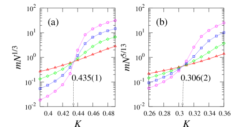
Figure 3: Plots of $mN^{\beta/\bar{\nu}}$ vs. $K$ for $\mu=5/19$ (a) and $\mu=5/13$ (b). The number of vertices $N$ is $10^{4}(\triangle)$, $10^{5}(\Diamond)$, $10^{6}(\square)$, and $10^{7}(\bigcirc)$. The data cross at $K_{c}=0.435(1)$ (a) and $K_{c}=0.306(2)$ (b), respectively, which are in accordance with $0.436$ and $0.305$ from Eq. (54).

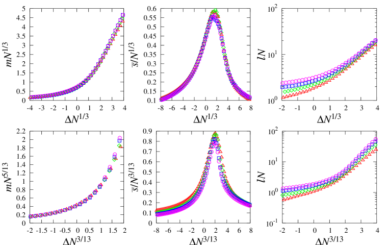
Figure 4: Data collapse of scaled giant cluster sizes $mN^{\beta/\bar{\nu}}$, mean cluster sizes $\bar{s}/N^{1/\bar{\nu}}$, and number of loops $\ell N$ plotted vs. $\Delta N^{1/\bar{\nu}}$ for $\mu=5/19$ (upper) and $\mu=5/13$ (lower). $N$ is $10^{4}(\triangle)$, $10^{5}(\Diamond)$, $10^{6}(\square)$, and $10^{7}(\bigcirc)$.

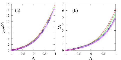
Figure 5: Data collapse of the scaled giant cluster size (a) and number of loops (b) vs. $\Delta$ for $\mu=5/7$. $N$ is $10^{4}(\triangle)$, $10^{5}(\Diamond)$, $10^{6}(\square)$, and $10^{7}(\bigcirc)$.

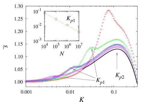
Figure 6: Mean cluster size $\bar{s}$ as a function of $K$ in semi-logarithmic scales with $\mu=5/7$ for $N=10^{4}(\triangle)$, $10^{5}(\Diamond)$, $10^{6}(\square)$, and $10^{7}(\bigcirc)$. In addition to the peak at $K_{p1}$, another peak is shown at $K_{p2}\simeq 0.1\,N$ for $N=10^{5}$, $10^{6}$, and $10^{7}$, respectively. The solid line represents the exact solution obtained from Eqs. (52) and (57). The measured values of $K_{p1}$ ($\bigcirc$) as a function of $N$ are plotted in the inset together with the guide line whose slope is $1-2\mu$ for comparison.

In this section, we derive the finite-size scaling forms of the giant cluster size $m$, the mean cluster size $\bar{s}$, and the number of loops $\ell$ and check against their numerical data from simulations for the static model. Investigating the cluster size distribution and the largest cluster size, we identified the critical regimes and the corresponding scaling variables, which enables us to predict the scaling behaviors of $m$, $\bar{s}$, and $\ell$.

Let us sketch the numerical procedure briefly. At each step, we pick two vertices $i$ and $j$, with probabilities $P_{i}$ and $P_{j}$, respectively. Then we put an edge between $i$ and $j$ unless there is one already. Repeat the procedure until there are $L$ edges made in the system. The generation of random numbers with non-uniform probability density $P_{i}$ is the most time-consuming part here. One efficient way is to use, e.g., Walker’s algorithm [26] combined with the so-called Robin Hood method [27], which is explained in Appendix B. This method is exact and takes time of ${\mathcal{O}}(N)$ to set up a table and ${\mathcal{O}}(1)$ to choose a vertex, making a large-size simulation feasible. Once a graph is constructed, the clusters are identified by the standard breadth-first search, during which we can extract the size of the largest cluster, the mean cluster size excluding the largest one as defined in Eq. (17), and the number of clusters within the graph. Recall that the number of clusters is related to the number of loops by Eq. (18). We choose three values of $\mu$, $\mu=5/19$ ($\lambda=4.8$), $5/13$ ($\lambda=3.6$), and $5/7$ ($\lambda=2.4$) as representatives of the regime (I), (II), and (III), respectively. We perform the simulations for the system size $N$ up to $10^{7}$, and the ensemble average is evaluated with at least $10^{3}$ runs.

Now we first consider the regime $0<\mu<1/2$ or $\lambda>3$. The scaling behaviors of the giant cluster size $m$ in this regime are shown in Eqs. (83) and (91) and can be written as

$$m=N^{-\frac{\beta}{\bar{\nu}}}\Psi_{\rm(I,II)}(\Delta N^{1\over\bar{\nu}}),$$ (98)

where the scaling exponents $\beta$ and $\bar{\nu}$ are given by

$$\beta = \left\{\begin{array}[]{ll}1&(0<\mu<\frac{1}{3}),\\ \frac{\mu}{1-2\mu}&(\frac{1}{3}<\mu<\frac{1}{2}),\end{array}\right.$$ (101)

$$\bar{\nu} = \left\{\begin{array}[]{ll}3&(0<\mu<\frac{1}{3}),\\ \frac{1}{1-2\mu}&(\frac{1}{3}<\mu<\frac{1}{2}).\end{array}\right.$$ (104)

The scaling function $\Psi_{\rm(I,II)}(x)$ behaves as

$$\Psi_{\rm(I,II)}(x)\sim\left\{\begin{array}[]{ll}{\rm const.}&(x\ll 1),\\ x^{\beta}&(x\gg 1).\end{array}\right.$$ (105)

The critical point $K_{c}$ can be found numerically by plotting $mN^{\beta/\bar{\nu}}$ vs. $K$ as shown in Fig. 3, which are in good agreement with Eq. (54). In Fig. 4, the plots of $mN^{\beta/\bar{\nu}}$ vs. $\Delta N^{1/\bar{\nu}}$ are shown for $\mu=5/19$ and $5/13$, respectively. The data collapse confirming the scaling behaviors in Eq. (98).

In the critical regime, the cluster size distribution follows the power law $P(s)\sim s^{-\tau}$ with $\tau=3/2$ for (I) and $1/(1-\mu)$ for (II). Then the mean cluster size in the critical regime is given by $\bar{s}\sim\langle S\rangle^{2-\tau}$ since $\bar{s}=\sum_{s\neq\langle S\rangle}sP(s)$. Since $\langle S\rangle\sim N^{1-\beta/\bar{\nu}}$ in the critical regime as in Eq. (98), the mean cluster size is represented as $\bar{s}\sim N^{(1-\beta/\bar{\nu})(2-\tau)}=N^{1/\bar{\nu}}$, which leads to, combined with Eq. (60),

$$\bar{s}=N^{1\over\bar{\nu}}\Phi_{\rm(I,II)}(\Delta N^{1\over\bar{\nu}}),$$ (106)

where the scaling function $\Phi_{\rm(I,II)}(x)$ behaves as

$$\Phi_{\rm(I,II)}(x)\sim\left\{\begin{array}[]{ll}{\rm const.}&(x\ll 1),\\ x^{-1}&(x\gg 1).\end{array}\right.$$ (107)

Plots of $\bar{s}/N^{1/\bar{\nu}}$ vs. $\Delta N^{1/\bar{\nu}}$ for $\mu=5/19$ and $5/13$ are shown in Fig. 4.

Since the giant cluster size and the mean cluster size correspond to the first and second derivative of the free energy with respect to the external field, respectively, it is natural that both have the same scaling variable. Therefore, the number of loops, corresponding to the free energy itself, is also described in terms of the scaling variable $\Delta N^{1/\bar{\nu}}$ with $\bar{\nu}$ in Eq. (104). Considering the number of loops for $K>K_{c}$ given in Eq. (66), one can see that

$$\ell={1\over N}\Omega_{\rm(I,II)}(\Delta N^{1\over\bar{\nu}}),$$ (108)

where the scaling function $\Omega_{\rm(I,II)}(x)$ behaves as

$$\Omega_{\rm(I,II)}(x)\sim\left\{\begin{array}[]{ll}{\rm const.}&(x\ll 1),\\ x^{\bar{\nu}}&(x\gg 1).\end{array}\right.$$ (109)

This implies that $\ell$ is $\mathcal{O}(N^{-1})$ in the critical regime, which is supported by the numerical simulation results in Fig. 4.

Next, we consider the regime $1/2<\mu<1$. From the largest cluster size shown in Eq. (97), the giant cluster size $m$ can be written as

$$m\sim N^{-\mu}~{}\Psi_{\rm(III)}(\Delta),$$ (110)

where the function $\Psi_{\rm(III)}(x)$ behaves as

$$\Psi_{\rm(III)}(x)\sim\left\{\begin{array}[]{ll}{\rm const.}&(x\ll 1),\\ x^{\mu\over 2\mu-1}&(x\gg 1).\end{array}\right.$$ (111)

Notice that $m$ increases smoothly passing $K_{c}(N)$ as manifested by $\Delta$ not scaling with $N$. Similarly, the number of loops $\ell$ represented in terms of the scaling variable $\Delta$ around $K_{c}(N)$ should exhibit the following scaling behaviors to satisfy Eq. (66):

$$\ell={1\over N}\Omega_{\rm(III)}(\Delta),$$ (112)

where the scaling function $\Omega_{\rm(III)}(x)$ behaves as

$$\Omega_{\rm(III)}(x)\sim\left\{\begin{array}[]{ll}{\rm const.}&(x\ll 1),\\ x^{1\over 2\mu-1}&(x\gg 1).\end{array}\right.$$ (113)

Data collapse of $mN^{\mu}$ and $\ell N$ vs. $\Delta$ is shown in Fig. 5.

The numerical data of the mean cluster size are shown in Fig. 6. As $N$ increases, the mean cluster size $\bar{s}$ approaches the exact solution in Eq. (57) represented by the solid line in Fig. 6. It does not diverge at any value of $K$, but instead its peak height decreases as $N$ increases. We additionally find that the mean cluster size $\bar{s}$ has a small peak at $K_{p1}$, which scales as $N^{1-2\mu}$ as shown in the inset of Fig. 6. The value of $K_{p1}$ is not equal to $K_{c}(N)$ although they are the same order of $N$. The reason for the peak at $K_{p1}$ is as follows. As $K$ increases, the largest cluster size $\langle S\rangle$ and the mean cluster size $\bar{s}=\sum_{s\neq\langle S\rangle}sP(s)$ also increase. However, as $K$ approaches $K_{c}(N)$, the cluster size distribution $P(s)$ begins to develop the exponential decaying part in its tail, i.e., for $s\gg s_{c}$. $s_{c}$ decreases with increasing $K$ after $K$ passes $K_{c}$. At $K_{p1}$, $\langle S\rangle$ and $s_{c}$ are equal. After $K$ passing $K_{p1}$, the mean cluster size is dominated by $s_{c}$, which makes $\bar{s}$ decrease for $K>K_{p1}$. However, the mean cluster size increases again as soon as $K$ becomes much larger than $K_{p1}$ or $K_{c}(N)$ because the prefactor $K^{1/\mu}$ of the cluster size distribution $P(s)$ for $1\ll s\ll s_{c}$ increases with increasing $K$. The mean cluster size decreases only after the second peak at $K_{p2}=\mathcal{O}(1)$, where $s_{c}=\mathcal{O}(1)$, as shown in Fig. 6 as well as in the exact solution in Fig. 2. Since $K_{p2}=\mathcal{O}(1)$, a giant cluster exists around $K_{p2}$.

8 Summary and Discussion

In this paper, we have studied the percolation transition of the SF random graphs constructed by attaching edges with probability proportional to the products of two vertex weights. By utilizing the Potts model representation, the giant cluster size, the mean cluster size, and the numbers of loops and clusters are obtained from the Potts model free energy in the thermodynamic limit. Our general formula for the giant cluster size and the mean cluster size are equivalent to those results obtained for a given degree sequence if the latter expressions are averaged over the grandcanonical ensemble. The Potts model formulation allows one to derive other quantities such as the number of loops easily. Using this approach, we then investigated the critical behaviors of the SF network realized by the static model in detail. Furthermore, to derive the finite size scaling properties of the phase transition, the cluster size distribution and the largest cluster size in finite size systems are also obtained and used. We found that there is a percolation transition for $\lambda=1+1/\mu>3$ so that a giant cluster appears abruptly when $K=\langle L\rangle/N$ is equal to $K_{c}$ given by Eq. (54) while such a giant cluster is generated gradually without a transition for $2<\lambda<3$. Thus the process of formation of the giant cluster for the case of $2<\lambda<3$ is fundamentally different from that of $\lambda>3$.

In particular, the difference between the SF graphs with $\lambda>3$ and $2<\lambda<3$ is manifested in the mean cluster size. For $\lambda>3$, as $K$ or the number of edges increases, many small clusters grow by attaching edges, which continues up to $K=K_{c}$, and then a giant cluster forms by the abrupt coalescence of those small clusters as shown in Fig. 7. Since we do not count the giant cluster in calculating $\langle s\rangle$, $\bar{s}$ decreases rapidly as $K$ passes $K_{c}$. Thus the mean cluster size exhibits a peak at $K=K_{c}$, which diverges in the thermodynamic limit $N\to\infty$. On the other hand, for $2<\lambda<3$, the role of $K_{c}$ is replaced by $K_{p1}$ which is $\sim{\mathcal{O}}(N^{-(3-\lambda)/(\lambda-1)})$, but after a small peak, the mean cluster size increases again after passing $K_{p1}$ as seen in Fig. 6: Edges newly introduced either create new clusters of size larger than $1$ or merge small clusters to the larger one with its size not as large as $\mathcal{O}(N)$. Only when $K$ reaches $K_{p2}$, the network is dense enough for the giant cluster to swallow up other clusters to reduce $\bar{s}$ on adding more edges. The evolution of the static model as the density of edges increases is summarized in Fig. 8.

Due to the characteristics of the power-law degree distribution of scale-free graphs, the cluster size distributions exhibit crossover behaviors such that they follow different power laws depending on the cluster size for given $\lambda$. In particular, for $3<\lambda<4$, the scaling exponents $\beta$ and $\bar{\nu}$ depend on the degree exponent $\lambda$ continuously while they are equal to the conventional mean-field values for $\lambda>4$. We have not considered the marginal cases where $1/\mu$ thus $\lambda$ is an integer value where logarithmic corrections appear as seen in Eq. (120).

Figure 7: Schematic picture for the comparison of cluster evolution between the case of $\lambda>3$ (a) and of $2<\lambda<3$ (b).

Figure 8: Schematic phase diagram of the static model. The SF behavior of the degree distribution appears between $K_{\ell}$ and $K_{u}$. A giant cluster emerges at $K_{c}$ for (I,II), and around $K_{p2}$ for (III). The quantities in $[\cdots]$ are only for (III).

The static model considered in this paper, though algebraically tractable, does not have correlations between edges that are important in real world networks. Extension of this work to the cases allowing correlations is left for the future work.

Appendix Appendix A The evaluation of $\Sigma_{1}(y)$

We derive the sums

$$\Sigma_{1}(y)\equiv{1\over N}\sum_{i=1}^{N}e^{-NP_{i}y},$$ (114)

where $P_{i}=i^{-\mu}/\zeta_{N}(\mu)$ $(0<\mu<1)$ with $\zeta_{N}(\mu)=\sum_{i=1}^{N}i^{-\mu}$ as in Eq. (45).

Let us introduce $y_{N}\equiv{N^{1-\mu}\over\zeta_{N}(\mu)}y$, which is equal to $(1-\mu)y$ in the thermodynamic limit $N\to\infty$ we are interested in. Then $\Sigma_{1}(y)=\sum_{i=1}^{N}s(i)$ with $s(x)=e^{-y_{N}(N/x)^{\mu}}/N$.

First consider the regime where $y_{N}N^{\mu}\ll 1$. Then $\Sigma_{1}(y)$ is simply expanded as

$$\Sigma_{1}(y) = {1\over N}\sum_{n=0}^{\infty}{(-1)^{n}\over n!}(y_{N}N^{\mu})^{n}\zeta_{N}(\mu n)$$ (115)

$$= \sum_{n=0}^{\lfloor\frac{1}{\mu}\rfloor}{(-1)^{n}\over n!(1-\mu n)}y_{N}^{n}+{1\over N}\sum_{n=\lfloor\frac{1}{\mu}+1\rfloor}^{\infty}{(-1)^{n}\over n!}(y_{N}N^{\mu})^{n}\zeta(\mu n),$$

with $\lfloor x\rfloor$ being the greatest integer less than or equal to $x$.

On the other hand, in the limit $y_{N}N^{\mu}\to\infty$, the second summation gives rise to a non-analytic term. Since $s(x)$ and its derivatives at $x=1$ and $x=N$ have the properties $s^{(n)}(1)=\mathcal{O}(N^{\mu n-1}e^{-y_{N}N^{\mu}})$ and $s^{(n)}(N)=\mathcal{O}(N^{-n-1})$ with $n\geq 0$, the Euler-Maclaurin formula [28] enables us to evaluate $\Sigma_{1}(y)$ in the limit $N\to\infty$ and $y_{N}N^{\mu}\to\infty$ as follows:

$$\Sigma_{1}(y) = \int_{1}^{N}dx\,s(x)=\int_{1}^{N}dx\,{1\over N}e^{-y_{N}\left(\frac{N}{x}\right)^{\mu}}$$ (116)

$$= {1\over\mu}y_{N}^{1\over\mu}\int_{y_{N}}^{\infty}dz\,z^{-1-\frac{1}{\mu}}e^{-z}$$

$$= {1\over\mu}y_{N}^{1\over\mu}\Gamma\left(-{1\over\mu},y_{N}\right),$$

where the incomplete Gamma function $\Gamma(s,x)$ is defined as

$$\Gamma(s,x)\equiv\int_{x}^{\infty}dt\,t^{s-1}e^{-t}.$$ (117)

The incomplete Gamma function can be expressed as

$$\Gamma(s,x) = \int_{x}^{\infty}dt\,t^{s-1}\left[e^{-t}-\sum_{n=0}^{\lfloor-s\rfloor}{(-t)^{n}\over n!}+\sum_{n=0}^{\lfloor-s\rfloor}{(-t)^{n}\over n!}\right]$$ (118)

$$= \int_{0}^{\infty}dt\,t^{s-1}\left[\sum_{n=\lfloor-s\rfloor+1}^{\infty}{(-t)^{n}\over n!}\right]$$

$$-\int_{0}^{x}dt\,t^{s-1}\left[\sum_{n=\lfloor-s\rfloor+1}^{\infty}{(-t)^{n}\over n!}\right]$$

$$+\int_{x}^{\infty}dt\,t^{s-1}\left[\sum_{n=0}^{\lfloor-s\rfloor}{(-t)^{n}\over n!}\right]$$

$$= \Gamma(s)-\sum_{n=0}^{\infty}{(-1)^{n}\over n!(s+n)}x^{n+s},$$

where it is used that $\Gamma(s)=\int_{0}^{\infty}dt\,t^{s-1}[e^{-t}-\sum_{n=0}^{\lfloor-s\rfloor}(-t)^{n}/n!]$, and therefore, it follows that

$$\Sigma_{1}(y)=\sum_{n=0}^{\infty}{(-1)^{n}\over n!(1-\mu n)}y_{N}^{n}-\Gamma\left(1-{1\over\mu}\right)y_{N}^{1\over\mu}.$$ (119)

As $\mu\to 1/m$ with $m$ an integer, a logarithmic term is developed as

$$\Sigma_{1}(y) =\sum_{n\neq m}^{\infty}{(-1)^{n}\over n!(1-\mu n)}y_{N}^{n}$$ (120)

$$+ {(-1)^{m}\over(m-1)!}y_{N}^{m}\left[-\ln y_{N}-\gamma_{M}+1+{1\over 2}+\cdots{1\over m-1}\right]$$

since

$$\lim_{\frac{1}{\mu}\to m}\left[{(-1)^{m}\over m!(1-\mu m)}y_{N}^{m}-\Gamma\left(1-{1\over\mu}\right)y_{N}^{1\over\mu}\right]$$

$$={(-y_{N})^{m}\over(1-\mu m)\Gamma(m+1)}\left[1-{1+(\frac{1}{\mu}-m)\ln y_{N}\over 1+{\Gamma^{\prime}(m)\over\Gamma(m)}(\frac{1}{\mu}-m)}\right]$$

$$={(-y_{N})^{m}\over(m-1)!}\left[-\ln y_{N}-\gamma_{M}+1+{1\over 2}+\cdots{1\over m-1}\right],$$ (121)

where it is used that $\Gamma(z)\Gamma(1-z)=\pi/\sin\pi z$ and $\Gamma^{\prime}(m)/\Gamma(m)=-\gamma_{M}+\sum_{n=1}^{\infty}[1/n-1/(n+m-1)]$.

Appendix Appendix B Walker algorithm

Suppose we want to choose discrete random numbers $x_{1},x_{2},\dots,x_{N}$, with probabilities $p_{1},p_{2},\dots,p_{N}$, respectively, where $p_{i}$’s are arbitrary yet properly normalized as $\sum_{i=1}^{N}p_{i}=1$. Walker algorithm enables one to choose $x_{i}$’s with appropriate frequencies by picking a single random number $0\leq r<1$. To do this, however, we have to set up a table $\{(q_{i},y_{i})\}$. The table is made in the following way.

1. Initialize $q_{i}$’s as $q_{i}=Np_{i}$, ($i=1,2,\dots,N$).

2. Divide $x_{i}$’s into the poor $(q_{i}<1)$ and the rich $(q_{i}>1)$.

3. Pick a poor, say $\mathbf{p}$, and a rich, say $\mathbf{r}$.

4. Fill the shortage of $\mathbf{p}$, $1-q_{\mathbf{p}}$, from $\mathbf{r}$.

5. $\mathbf{p}$ records the donator $\mathbf{r}$ as $y_{\mathbf{p}}=\mathbf{r}$.

6. $q_{\mathbf{r}}$ is updated as $q_{\mathbf{r}}\leftarrow q_{\mathbf{r}}-(1-q_{\mathbf{p}})$.

7. If ${\mathbf{r}}$ becomes poor by the donation, i.e., $q_{\mathbf{r}}<1$, $\mathbf{r}$ enters the list of the poor out of that of the rich.

8. Repeat $(3)$–$(7)$ until there are no poor left (hence the name Robin Hood method).

The donate-and-fill steps $(3)$–$(7)$ are performed at most $N-1$ times, thus the table-making procedure takes time of $\mathcal{O}(N)$. In its original introduction [26], Walker proposed the step $(3)$ as “pick the poorest and the richest,” which involves additional sorting operation, increasing the computational cost. The present scheme follows the implementation of Zaman [27]. The table-making process can be visualized for a simple $N=3$ case as in Fig. B.9.

Figure B.9: Illustration of the table-making procedure in the Walker algorithm for $N=3$. The heights of the white bars in (c) indicates $q_{i}/N$ and the figures in the shaded boxes $y_{i}$.

With the table $\{(q_{i},y_{i})\}$ at hand, one picks a random number $0\leq r<1$. Divide $x=rN+1$ into the integer part $n=\lfloor x\rfloor$ and the remainder $d=x-n$. If $d<q_{n}$, we choose $x_{n}$, otherwise choose $y_{n}$. With this scheme one can draw discrete random numbers $x_{i}$’s with appropriate probabilities $p_{i}$’s.

References

- [1] P. Erdős and A. Rényi, Publ. Math. Inst. Hung. Acad. Sci. 5, 17 (1960); Bull. Inst. Int. Stat. 38, 343 (1961).
- [2] A.-L. Barabási and R. Albert, Science 286, 509 (1999).
- [3] R. Albert and A.-L. Barabási, Rev. Mod. Phys. 74, 47 (2002).
- [4] S. N. Dorogovtsev and J. F. F. Mendes, Adv. Phys. 51, 1079 (2002).
- [5] M. E. J. Newman, SIAM Rev. 45, 167 (2003).
- [6] J. Berg and M. Lässig, Phys. Rev. Lett. 89, 228701 (2002).
- [7] M. Baiesi and S. S. Manna, Phys. Rev. E 68, 047103 (2003).
- [8] Z. Burda, J. D. Correia, and A. Krzywicki, Phys. Rev. E 64, 046118 (2001); Z. Burda and A. Krzywicki, Phys. Rev. E 67, 046118 (2003).
- [9] S. N. Dorogovtsev, J. F. F. Mendes, and A. N. Samukhin, Nucl. Phys. B 666, 396 (2003).
- [10] I. Farkas, I. Derenyi, G. Palla, and T. Viscek, in Lecture notes in Physics: Networks: structure, dynamics, and function, edited by E. Ben-Naim, H. Frauenfelder, and Z. Toroczkai (Springer, 2004).
- [11] M. Molloy and B. Reed, Random Struct. Algorithms 6, 161 (1995); Combinatorics, Probab. Comput. 7, 295 (1998).
- [12] M. E. J. Newman, S. H. Strogatz, and D. J. Watts, Phys. Rev. E 64, 026118 (2001).
- [13] K.-I. Goh, B. Kahng, and D. Kim, Phys. Rev. Lett. 87, 278701 (2001).
- [14] G. Caldarelli, A. Capocci, P. De Los Rios, and M. A. Muñoz, Phys. Rev. Lett. 89, 258702 (2002).
- [15] B. Söderberg, Phys. Rev. E 66, 066121 (2002).
- [16] F. Chung and L. Lu, Annals Combinatorics 6, 125 (2002).
- [17] W. Aiello, F. Chung, and L. Lu, Exp. Math. 10, 53 (2001).
- [18] P. W. Kasteleyn and C. M. Fortuin, J. Phys. Soc. Japan Suppl. 16, 11 (1969); C. M. Fortuin and P. W. Kasteleyn, Physica 57, 536 (1972). Also see F. Y. Wu, Rev. Mod. Phys. 54, 235 (1982).
- [19] S. N. Dorogovtsev, A. V. Goltsev, and J. F. F. Mendes, cond-mat/0310693.
- [20] R. Cohen, K. Erez, D. ben-Avraham, and S. Havlin, Phys. Rev. Lett. 85, 4626 (2000); Phys. Rev. Lett. 86, 3682 (2001).
- [21] D. S. Callaway, M. E. J. Newman, S. H. Strogatz, and D. J. Watts, Phys. Rev. Lett. 85, 5468 (2000).
- [22] R. Cohen, D. ben-Avraham, and S. Havlin, Phys. Rev. E 66, 036113 (2002).
- [23] R. Otter, Ann. Math. Statist. 20, 206 (1949); T. E. Harris, The Theory of Branching Processes (Dover, New York, 1989).
- [24] D. Stauffer and A. Aharony, Introduction to percolation theory (Taylor & Francis, London, 1992).
- [25] R. Cohen, S. Havlin, and D. ben-Avraham, in Handbook of Graphs and Networks, edited by S. Bornholdt and H.G. Shuster (Willey-VCH, New York, 2002), Chap. 4.
- [26] A. J. Walker, Electron. Lett. 10, 127 (1974).
- [27] A. Zaman, unpublished manuscript (1996).
- [28] G. Arfken, Mathematical methods for physicists (Academic, Orlando, 1985).