The internal Josephson effect in a Fermi gas near a Feshbach resonance

Abstract

We consider a two-component system of Fermi atoms and molecular bosons in the vicinity of a Feshbash resonance. We derive an effective action for the system, which has a term describing coherent tunneling of the molecular bosons into Cooper pairs and vice versa. In the equilibrium state, global phase coherence may be destroyed by thermal or quantum phase fluctuations. In the non-equilibrium regime, the system may show an internal AC Josephson effect leading to real time oscillations in the number of molecular bosons.

Introduction. Trapped dilute cold Fermi systems Levi (2003); Cho (2003) are one of the most exciting areas of research in modern condensed matter physics. This field offers a great variety of novel phenomena Donley et al. (2002); Regal et al. (2004a); Zwierlein et al. (2004); Regal et al. ; Regal et al. (2004b); Regal and Jin (2003) and presents serious challenges for both experimentalists and theorists. The magnetic-field induced Feshbach resonance Timmermans et al. (1999) provides an unprecedented degree of control over the inter-particle interactions as well as the rate at which the interactions are changed. By sweeping magnetic field, one can tune the sign and the strength of the interaction Regal and Jin (2003) and experimentally access the BCS-BEC crossover physics Nozières and Schmitt-Rink (1985). Apart from this, by adjusting the sweeping rate, one can drive the system into various non-equilibrium states in which different bosonic and fermionic species co-exist and interact with each other.

Interaction between fermions consists of two channels: an inelastic channel involving the formation of a molecular state of two fermions and a resonant elastic scattering channel. Typically, the elastic scattering length is an unremarkable function of the applied field. However, in the vicinity of a certain value of the field $B_{0}$, the scattering length changes dramatically Timmermans et al. (1999); Regal and Jin (2003). On the BEC side of the Feshbach resonance, the molecular energy level is located below the continuum states and the molecular state is stable. On the BCS side of the resonance, high magnetic field breaks up the molecular states and one would expect that the molecular component vanish. However, recent experimental results Regal et al. (2004b) and theoretical works Ohashi and Griffin ; Falco and Stoof (2004) suggest that even on the BCS side of the resonance, the fraction of molecular states is non-zero. One may assume the existence of an energy barrier between the molecular state and the continuum and so the molecular state on the BCS side of the resonance may actually be metastable. This may happen in part due to a stabilizing effect of the Fermi liquid coupled to the molecular component. In turn, the molecular component affects the fermionic degrees of freedom renormalizing effective fermion-fermion interactions Ohashi and Griffin ; Stajic et al. .

At low temperatures, attractive interaction between fermions should lead to the formation of Cooper pairs Bohn (2000); Regal et al. (2004a); Zwierlein et al. (2004). The condensate of Cooper pairs would co-exist and interact with the system of preformed molecular bosons if the life-time of the molecular state is long enough. It is interesting to describe the co-existence of the two coherent states, and this issue is the main subject of the present work. In this Letter, we study theoretically a Fermi-Bose mixture and discuss quasiequilibrium and non-equilibrium properties of the system.

We start with an effective low energy Hamiltonian describing the system near the resonance (on the high-field BCS side) Holland et al. (2001); Duine and Stoof . In this Hamiltonian, the resonant and non-resonant processes are separated by introducing an effective Feshbach coupling of the fermion component to the metastable molecular field. We integrate out the one-particle fermionic degrees of freedom and explicitly derive an effective action for the system. This action contains a term which can be interpreted as an internal Josepshon tunneling Leggett (2001) of molecular bosons into Cooper pairs and vice versa. The action also contains a “charging energy” term, describing phase diffusion. In the quasiequilibrium regime, phase coherence between the two states can be destroyed by either temperature or quantum phase fluctuations. We explicitly derive the crossover line, which is a function of the number of particles in the system $N$. In the limit $N\to\infty$, the internal DC Josephson effect is dominant and global phase coherence is established in the system.

We also discuss a non-equilibrium situation by considering a non-adiabatic sweep of the magnetic field across the resonance. We predict that under certain circumstances, the system may exhibit Josephson AC oscillations. In this case, the numbers of molecular bosons and Cooper pairs oscillate in real time, slowly relaxing to a stationary state, which depends on the magnetic field sweeping rate. In addition, we discuss relevant time-scales at which such a relaxation takes place.

Effective action. Let us consider a system of Fermi atoms with two hyperfine states labeled with the index $\sigma=\uparrow,\,\downarrow$. The effective Hamiltonian for the system in the vicinity of the Feshbach resonance has the following form Holland et al. (2001):

$${\cal H}-\mu N=\int d^{3}{\bf r} \!\!\!\!\!\Biggl{\{}\psi^{\dagger}_{\sigma}\left({\bf r}\right)\left[-{\nabla^{2}\over 2m}-\mu\right]\psi_{\sigma}\left({\bf r}\right)$$

$$-{U\over 2}\psi^{\dagger}_{\sigma}\left({\bf r}\right)\psi^{\dagger}_{-\sigma}\left({\bf r}\right)\psi_{-\sigma}\left({\bf r}\right)\psi_{\sigma}\left({\bf r}\right)$$

$$+\phi^{\dagger}\left({\bf r}\right)\left[-{\nabla^{2}\over 2M}+\delta-2\mu\right]\phi\left({\bf r}\right)$$

$$+g\left[\phi^{\dagger}\left({\bf r}\right)\psi_{\sigma}\left({\bf r}\right)\psi_{-\sigma}\left({\bf r}\right)+\mbox{h.c.}\right]\Biggr{\}},$$

where $\psi$ and $\phi$ are field operators for fermions and molecular bosons respectively, $U$ is the fermion-fermion interaction strength, $\delta\sim 2\mu_{\rm B}\left(B-B_{0}\right)$ is the detuning from the resonance, $g$ is the Feshbach coupling between molecular bosons and fermions (which is connected with the width of the resonance $\Delta B$ Duine and Stoof ), and $m$ and $M$ are fermionic and molecular masses respectively.

The grand partition function for the system is

$$Z_{G}={\rm Tr}\,\exp\left[-\beta\left({\cal H}-\mu N\right)\right],$$ (2)

where the trace is taken over the fermionic and bosonic degrees of freedom. Now let us introduce the Hubbard-Stratonovich field $\Delta$ to decouple the four-fermion term $H_{U}$ in the action, which can be re-written in the following form

$$T_{\tau}\,\exp\left[-\int\limits_{0}^{\beta}d\tau H_{U}(\tau)\right]=\,\int{\cal D}^{2}\Delta(x)e^{\left[-U^{-1}\int dx\left|\Delta(x)\right|^{2}\right]}$$

$$\,\,\,\,\,\,\,\,\,\,\,\,\,\,\,\,\,\,\times T_{\tau}\exp\left[-\int dx\left\{\Delta(x)\psi^{\dagger}_{\sigma}(x)\psi^{{}^{\dagger}}_{-\sigma}(x)+\mbox{h.c.}\right\}\right],$$ (3)

where we introduced $x=\left(\tau,{\bf r}\right)$ for the sake of brevity. Let us note that the last term in Eq. (The internal Josephson effect in a Fermi gas near a Feshbach resonance) is very similar to the Feshbach coupling term in Eq. (The internal Josephson effect in a Fermi gas near a Feshbach resonance). To proceed further, let us evaluate the Gaussian integral over the fermionic degrees of freedom in the spirit of Ref. Ambegaokar et al. (1982). We use the following standard Nambu notations:

$$\hat{\psi}(x)={\psi_{\uparrow}(x)\choose\psi^{\dagger}_{\downarrow}(x)}.$$

The Hubbard-Stratonovich and molecular fields read

$$\hat{\Delta}(x)=\left(\begin{array}[]{cc}0&\Delta(x)\\ \Delta^{*}(x)&0\end{array}\right)\,\,\,\mbox{and}\,\,\,\hat{\phi}(x)=\left(\begin{array}[]{cc}0&\phi(x)\\ \phi^{*}(x)&0\end{array}\right).$$

The Green’s function $\hat{G}(x)=-\left\langle T_{\tau}\,\hat{\psi}(x)\hat{\psi}^{\dagger}(x)\right\rangle$ is also a $2\times 2$ matrix. In the Nambu notations, the grand partition function takes the following form:

$$Z_{G}=\int{\cal D}^{2}\Delta(x)\,{\cal D}^{2}\phi(x)\exp\left\{-S_{\rm eff}\left[\hat{\Delta},\hat{\phi}\right]\right\},$$ (4)

where the effective action can be written in the compact form:

$$S_{\rm eff}\left[\hat{\Delta},\hat{\phi}\right]= \!\!\int\limits_{0}^{\beta}d\tau{\cal H}^{(0)}_{\phi}(\tau)+{1\over U}\int dx\left|\Delta(x)\right|^{2}$$ (5)

$$\!\!\!\!-{\bf{\rm Tr}}\left[\ln\hat{G}_{0}^{-1}+\ln\hat{G}^{-1}\right].$$

Where the trace is over the spatial and time variables and Nambu indices and ${\cal H}^{(0)}_{\phi}$ is the Hamiltonian of the system of molecular bosons (without the Feshbach coupling). The matrix Green’s function (which quite generally is a functional of the pairing and bosonic fields) is the solution of the following equation:

$$\left[-{\partial\over\partial\tau}\hat{1}-\left(-{\nabla^{2}\over 2m}-\mu\right)\hat{\sigma}_{3}-\hat{\Delta}(x)-g\hat{\phi}(x)\right]\hat{G}\left(x,x^{\prime}\right)$$

$$=\delta(t-t^{\prime})\,\delta({\bf r}-{\bf r}^{\prime}),$$ (6)

where $\hat{\sigma}_{\alpha}$ is the Pauli matrix in the Nambu space.

In what follows, we consider a homogeneous order parameter. This approximation is exact in the zero-dimensional case, i. e. when the size of the system is smaller than the coherence length, otherwise one should study Ginzburg-Landau equations taking into account the spatial dependence of the fields.

Both the pairing field and the Bose-field are complex functions of the imaginary time. Let us write them in the form:

$$\Delta(\tau)=\Delta_{0}e^{i\chi_{1}(\tau)}\,\,\,\mbox{and}\,\,\,\phi(\tau)=\phi_{0}\,e^{i\chi_{2}(\tau)}$$

and perform the following gauge transformation

$$\hat{\tilde{\psi}}(x)=\left(\begin{array}[]{cc}e^{-i\chi_{1}(\tau)/2}&0\\ 0&e^{i\chi_{1}(\tau)/2}\end{array}\right)\hat{\psi}(x).$$

In this gauge, the Green’s function reads (although the coordinate dependences of the order parameters are neglected, the Green’s function depends on ${\bf r}$ and ${\bf r}^{\prime}$):

$$\left[-{\partial\over\partial\tau}\hat{1}-\left(-{\nabla^{2}\over 2m}-\mu\right)\hat{\sigma}_{3}-\hat{\Delta}_{0}-g\hat{\tilde{\phi}}(\tau)-{i\over 2}{\partial\chi_{1}\over\partial\tau}\hat{\sigma}_{3}\right]$$

$$\times\hat{\tilde{G}}\left(\tau,\tau^{\prime};{\bf r}-{\bf r}^{\prime}\right)=\delta(t-t^{\prime})\,\delta({\bf r}-{\bf r}^{\prime}).$$ (7)

Where the new bosonic field (the order parameter describing a superfluid phase of molecular bosons) is given by

$$\hat{\tilde{\phi}}=\phi_{0}\left(\begin{array}[]{cc}0&e^{i\left(\chi_{2}-\chi_{1}\right)}\\ e^{i\left(\chi_{1}-\chi_{2}\right)}&0\end{array}\right).$$

Now, let us consider the case when the bosonic and dynamic terms in the Green’s function are small compared to the other terms. In this limit, the effective action can be expanded with respect to the small terms:

$$S_{\rm eff}\left[\hat{\Delta},\hat{\phi}\right]= \!\!\!\!\!-\,{\bf{\rm Tr}}\left[\ln\hat{G}_{0}^{-1}-\ln\hat{G}_{\rm GN}^{-1}\right]+{V\beta\over U}\Delta_{0}^{2}$$ (8)

$$\!\!\!\!\!+\int\limits_{0}^{\beta}d\tau{\cal H}^{(0)}_{\phi}(\tau)+\,{\bf{\rm Tr}}\left[\hat{G}_{\rm GN}\left(g\hat{\phi}+{i\over 2}{\partial\chi_{1}\over\partial\tau}\hat{\sigma}_{3}\right)\right]$$

$$\!\!\!\!\!+\,{\bf{\rm Tr}}\left[\hat{G}_{\rm GN}\left(g\hat{\phi}+{i\over 2}{\partial\chi_{1}\over\partial\tau}\hat{\sigma}_{3}\right)\right]^{2}+\ldots,$$

where $\hat{G}_{\rm GN}$ is the Gor’kov-Nambu Green’s function matrix:

$$\hat{G}_{\rm GN}(\tau,{\bf r})=\left(\begin{array}[]{cc}G(\tau,{\bf r})&F(\tau,{\bf r})\\ F(\tau,{\bf r})&-G(-\tau,-{\bf r})\end{array}\right).$$ (9)

In the momentum representation, the components of the matrix have the following well-known form Abrikosov et al. (1990):

$$G\left(\varepsilon_{n},{\bf p}\right)=-{\xi_{p}+i\varepsilon_{n}\over\Delta_{0}^{2}+\xi_{p}^{2}+\varepsilon^{2}}\,\,\,\mbox{and}\,\,\,F\left(\varepsilon_{n},{\bf p}\right)={\Delta_{0}\over\Delta_{0}^{2}+\xi_{p}^{2}+\varepsilon_{n}^{2}},$$ (10)

where $\epsilon_{n}=\left(2n+1\right)\pi T$ is the fermionic Matsubara frequency. The first two terms in action (8) pin the mean-field value of the BCS order parameter, while the third term controls the magnitude of the superfluid molecular field [in principle one can include higher order terms with respect to $\phi$ in the initial Hamiltonian (The internal Josephson effect in a Fermi gas near a Feshbach resonance), describing interactions between molecules; the tunneling terms in the action will remain the same in this case]. The most interesting contributions come from the fourth and fifth terms in Eq. (8), which describe quantum phase dynamics. Using Eqs. (8), (9), and (10), we obtain the first order correction to the mean-field action:

$$\delta S_{1}={\rm Tr\,}\left[\hat{G}_{\rm GN}{\partial\chi_{1}\over\partial\tau}\hat{\sigma}_{3}\right]=-J\int\limits_{0}^{\beta}d\tau\cos\left[\chi_{1}\left(\tau\right)-\chi_{2}\left(\tau\right)\right],$$ (11)

with

$$J(T)={3\over 2}N{g\phi_{0}(T)\Delta_{0}(T)\over\epsilon_{\rm F}}\ln{\left[\tilde{\epsilon}\over{\rm max}\,\left\{\Delta_{0}(T),T\right\}\right]},$$ (12)

where $N$ is the number of particles in the Fermi system, $\epsilon_{\rm F}$ is the Fermi energy, and $\tilde{\epsilon}$ is the BCS high-energy cut-off (in our case $\tilde{\epsilon}\sim\epsilon_{\rm F}$). The leading contribution coming from the second order correction term [the last term in Eq. (8)] generally has a complicated non-local form. However, if the phase dynamics is slow enough at the time-scale $\Delta_{0}^{-1}$, the action can be reduced to the familiar local form:

$$\delta S_{2}={1\over 8E_{\rm C}}\int\limits_{0}^{\beta}d\tau\left({\partial\chi_{1}\over\partial\tau}\right)^{2},$$ (13)

where

$$E_{\rm C}^{-1}(T)={3c(T)\over 2}{N\over\epsilon_{\rm F}}$$ (14)

and the function $c(T)$ is given by

$$c(T)=\int\limits_{-{\infty}}^{\infty}d\xi\left\{{\Delta_{0}^{2}(T)\over E^{3}}\tanh\left[{E\over 2T}\right]-{\xi^{2}\over 4TE^{2}}\cosh^{-2}\left[{E\over 2T}\right]\right\},$$ (15)

with $E=\sqrt{\Delta_{0}^{2}(T)+\xi^{2}}$. This function has the following asymptotic behavior at low and high temperatures: $c(T\ll\Delta_{0})=1$ and $c(T\gg\Delta_{0})\approx\pi\Delta_{0}(T)/T$. Summarizing, let us present the main technical result of the present work:

$$\delta S=\int\limits_{0}^{\beta}d\tau\left[-J\cos\left[\chi_{1}\left(\tau\right)-\chi_{2}\left(\tau\right)\right]+{1\over 8E_{\rm C}}\left({\partial\chi_{1}\over\partial\tau}\right)^{2}\right],$$ (16)

where the parameters $J$ and $E_{C}$ are given by Eqs. (12) and (14). The first term in action (16) can be easily recognized as a Josephson term, which describes coherent tunneling of the molecular bosons into the condensate of fermionic Cooper pairs and vice versa. Unlike in the conventional Josephson effect Josephson (1962), the two quantum states are not separated by any physical energy barrier being mixed up in the real space Leggett (2001). The second term in Eq. (16) is the effective “charging energy.” This term describes quantum phase fluctuations. In a neutral superfluid, phase dynamics is possible only due to the finite size of the system (this is different from the case of a superconducting junction, when quantum phase fluctuations are possible in any system of finite capacitance).

Quasiequilibrium regime. Let us consider first a system of Cooper pairs and preformed molecular bosons in the thermodynamic equilibrium, i. e. $\dot{\phi}=0$. In this state, the molecular order parameter is directly related to the BCS order parameter Chiofalo et al. (2002). The corresponding relation follows from the condition $\left[\phi,{\cal H}\right]=0$ and Eq. (The internal Josephson effect in a Fermi gas near a Feshbach resonance):

$$\phi_{0}={g\over 2\mu-\delta}{\Delta_{0}\over U}.$$ (17)

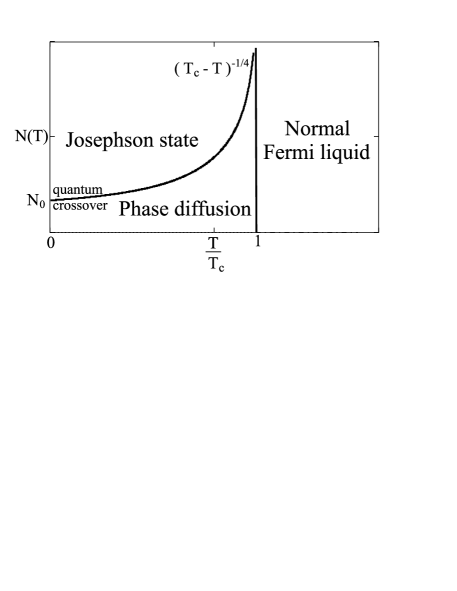
Figure 1: This diagram describes a crossover between the phase coherent Josephson dynamics and the phase oscillating (Fock) regime. The curve shows the critical number of particles as a function of temperature at which the crossover occurs.

In the quasiequilibrium regime, the internal Josephson effect tends to establish phase coherence between the two condensates. However, even at zero temperature, this coherence can be destroyed by quantum phase fluctuations due to a finite mass term in the action (16). A crossover between the semiclassical Josephson dynamics and quantum phase diffusion occurs when Raghavan et al. (1999) $J\sim E_{\rm C}$. From this condition and Eqs. (12), (14), and (17) (at zero temperature), we derive the following expression for the number of particles in the Fermi liquid corresponding to the quantum crossover point:

$$N_{\rm c}(0)\sim\left[{\nu_{\rm F}U^{2}\left(\delta-2\mu\right)\over g^{2}}\right]^{1/2}e^{1/\left(\nu_{\rm F}U\right)},$$ (18)

where $\nu_{\rm F}$ is the density of states at the Fermi level and we have used the BCS formula for the transition temperature with $\epsilon_{\rm F}$ as a high-energy cut-off. We emphasize that the effect can not be called a quantum phase transition, since the transition is driven by finite size of the system and disappears in the thermodynamic limit (the system is always in the phase coherent state if $N=\infty$). At finite temperatures, the Josephson effect is suppressed by thermal fluctuations. The corresponding crossover between the coherent state of two condensates and random phase rotation can be estimated from the relation $J(T)\sim E_{\rm C}(T)$, using Eqs. (12) and (14):

$$N_{\rm c}(T)\sim N_{\rm c}(0)\sqrt{c(T)}{\Delta_{0}\over\Delta_{0}(T)},$$ (19)

where the function $c(T)$ is given by Eq. (15) and $\Delta_{0}(T)$ is the temperature dependent BCS gap Abrikosov et al. (1990). The $N_{\rm c}(T)$-dependence was evaluated numerically and the corresponding curve is shown in Fig. 1.

Non-equilibrium dynamics. Let us consider a non-equilibrium case, when a magnetic field is swept suddenly from the BEC to the BCS side of the resonance. In this case one has a non-equilibrium situation: the distribution function of quasiparticles $f({\bf k})$ is not given by the familiar equilibrium distribution $f_{0}({\bf k})=\left[1+\exp\left(\beta\sqrt{\xi_{\bf k}^{2}+\Delta^{2}}\right)\right]^{-1}$. The technique used previously is formally valid only if the time-scale at which the order parameter changes is much larger than the quasiparticle relaxation rate $\tau_{\Delta}\gg\tau_{\epsilon}$. This is definitely true in the close vicinity of the transition point [$\Delta\ll T_{c}\sim\Delta(T=0)$]: $\tau_{\Delta}\sim\tau_{\varepsilon}{T_{c}/\Delta}\gg\tau_{\varepsilon}$, where $\tau_{\epsilon}^{-1}$ is the quasiparticle relaxation rate, which in a clean Fermi liquid can be estimated as $\tau_{\epsilon}^{-1}\sim\nu_{\rm F}UT^{2}/\epsilon_{\rm F}$. However, away from the transition point, the domain of applicability of the theory presented earlier is determined by the following condition: $\Delta\ll\nu_{\rm F}UT^{2}/\epsilon_{\rm F}$. At very low temperatures, the quasiparticle distribution function cannot follow the changes of the pairing field; to describe such a non-equilibrium regime, it is necessary to use the Keldysh technique Larkin and Ovchinnikov (1984) or study the equations of motion for the superfluid phase (Josephson equations) coupled to the kinetic equations for the one particle distribution function. Unfortunately, the corresponding derivation is quite cumbersome (and will be published elsewhere). Below, we present only qualitative results discussing several non-equilibrium regimes possible in the system of interest:

It is natural to assume that by sweeping the magnetic field across the resonance, we elevate the chemical potential of the bosonic component relative to the chemical potential of the BCS condensate Eds., D. N. Langenberg and Larkin (1986). The corresponding chemical potential difference $\delta$ yields an effect similar to the effect of voltage in superconducting junctions. Therefore, if $\delta\ll 2\Delta$ the system should exhibit oscillations associated with an internal AC Josephson effect:

$$\dot{N}_{\rm b}=J\sin{\left(\delta t+\phi_{0}\right)}.$$ (20)

These oscillations correspond to coherent tunneling back and forth between the two quantum states (condensates of molecular bosons and Cooper pairs). Due to the AC Josephson effect, the number of molecular bosons would oscillate in real time and this behavior should in principle be observable in experiment Donley et al. (2002) with the help of the radio-frequency spectroscopy technique Levi (2003).

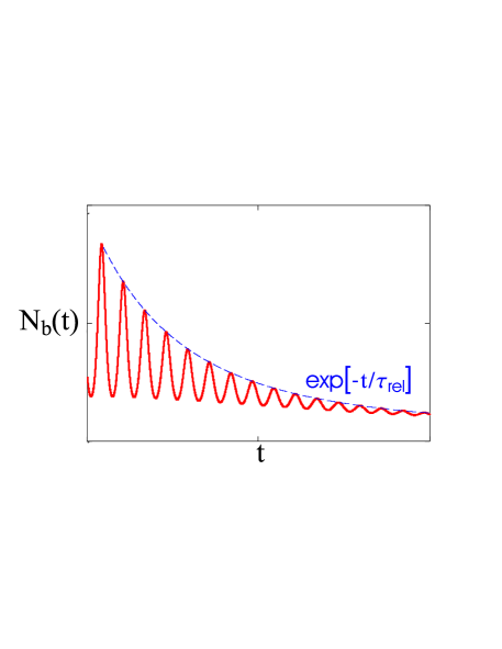
Figure 2: Real time dynamics of the number of molecular bosons in the Josephson regime: $\delta\ll 2\Delta$. The solid curve shows AC Josephson oscillations in the number of particles. The oscillations decay with time and the system tends to an equilibrium state, which generally depends upon the magnetic field sweeping rate.

A different physical picture emerges when we consider the regime of a highly excited molecular state with $\delta\gg 2\Delta$. In this limit, the molecular bosons quickly dissociate into one-particle excitations and the Josephson effect disappears. In this case, one would expect to observe Rabi oscillations, which were described in details in Ref. Barankov et al. for a generic BCS problem.

The internal AC Josephson dynamics described above and the Rabi oscillations of Ref. Barankov et al. are dissipationless, since equilibration is possible only in the presence of relaxation processes in the system of one-particle excitations. If the temperature is low enough (keeping in mind that the word “temperature” has somewhat ambiguous meaning in a non-equilibrium case) the relaxation to a final equilibrium state is quite slow (see Fig. 2) and the corresponding relaxation rate is likely to be exponentially small: $\tau_{\rm rel}^{-1}\sim\tau_{\varepsilon}^{-1}\exp{\left[-{{\rm min\,}\left\{\delta,\Delta\right\}/T_{\rm i}}\right]}$, where $T_{\rm i}$ is the initial temperature before the magnetic field sweep.

Another important question concerns the final equilibrium state to which the system relaxes at $t\to\infty$. This state depends on the final temperature $T_{\rm f}$ of the system. The latter is related to the details of the magnetic field sweep. By rapidly (nonadiabatically) changing the magnetic field, one puts the system in an excited state Barankov et al. ; Eliashberg ; in the process of relaxation, the system heats up being unable to drain the extra energy. The temperature change relates to the energy pumping rate $\dot{\delta}\sim 2\mu_{\rm B}\left({\partial B/\partial t}\right)$ Barankov et al. ; Eliashberg . If the final temperature is higher than the superconducting transition temperature $T_{\rm f}>T_{\rm c}$, the equilibrium phase of the system is a normal Fermi liquid state; in the opposite limit $T_{c}<T_{\rm f}$, the system relaxes toward a quasistationary state, which is either the Josephson coherent state [if the system is large enough, $N>N_{\rm c}(T_{\rm f})$; see Eq. (19) and Fig. 1] or the Fock state [if $N<N_{\rm c}(T_{\rm f})$].

Acknowledgements. The author is very grateful to Anatoly Larkin for his extremely helpful comments and to Donald Priour Jr. for reading the manuscript. The author also acknowledges stimulating discussions with Roman Barankov. The work was supported by the US-ONR, LPS, and DARPA.

References

- Levi (2003) B. G. Levi, Phys. Today 56, 20 (2003).
- Cho (2003) A. Cho, Science 301, 750 (2003).
- Donley et al. (2002) E. A. Donley, N. R. Claussen, S. T. Thompson, and C. E. Wieman, Nature 417, 529 (2002).
- Regal et al. (2004a) C. A. Regal, M. Greiner, and D. S. Jin, Phys. Rev. Lett. 92, 040403 (2004a).
- Zwierlein et al. (2004) M. W. Zwierlein, C. A. Stan, C. H. Schunck, S. M. F. Raupach, A. J. Kerman, and W. Ketterle, Phys. Rev. Lett. 92, 120403 (2004).
- (6) C. Regal, C. Ticknor, J. L. Bohn, and D. S. Jin, Nature 424, 47 (2003); M. Greiner, C. A. Regal, and D. S. Jin, Nature 426, 537 (2003).
- Regal et al. (2004b) C. A. Regal, M. Greiner, and D. S. Jin, Phys. Rev. Lett. 92, 083201 (2004b).
- Regal and Jin (2003) C. A. Regal and D. S. Jin, Phys. Rev. Lett. 90, 230404 (2003).
- Timmermans et al. (1999) E. Timmermans, P. Tommasini, M. Hussein, and A. Kerman, Phys. Rep. 315, 199 (1999).
- Nozières and Schmitt-Rink (1985) P. Nozières and S. Schmitt-Rink, J. Low. Temp. Phys. 59, 195 (1985).
- (11) Y. Ohashi and A. Griffin, Phys. Rev. Lett. 89, 130402 (2002); Phys. Rev. A 67, 1050 (2003).
- Falco and Stoof (2004) G. M. Falco and H. T. C. Stoof, Phys. Rev. Lett. 92, 130401 (2004).
- (13) J. Stajic, J. N. Milstein, Q. Chen, M. L. Chiofalo, M. J. Holland, and K. Levi, cond-mat/0309329.
- Bohn (2000) J. L. Bohn, Phys. Rev. A 61, 053409 (2000).
- Holland et al. (2001) M. Holland, S. J. J. M. F. Kokkelmans, M. L. Chiofalo, and R. Walser, Phys. Rev. Lett. 87, 120406 (2001).
- (16) R. A. Duine and H. T. C. Stoof, cond-mat/0312254.
- Leggett (2001) A. J. Leggett, Rev. Mod. Phys. 73, 307 (2001).
- Ambegaokar et al. (1982) V. Ambegaokar, U. Eckern, and G. Schn, Phys. Rev. Lett. 48, 1745 (1982).
- Abrikosov et al. (1990) A. A. Abrikosov, L. P. Gor’kov, and I. Y. Dzyaloshinskiî, Quantum field theorectical methods in statistical physics (Pergamon Press, New York, 1990).
- Josephson (1962) B. D. Josephson, Phys. Lett. 1, 251 (1962).
- Chiofalo et al. (2002) M. L. Chiofalo, S. J. J. M. F. Kokkelmans, J. N. Milstein, and M. J. Holland, Phys. Rev. Lett. 88, 090402 (2002).
- Raghavan et al. (1999) S. Raghavan, A. Smerzi, S. Fantoni, and S. R. Shenoy, Phys. Rev. A 59, 620 (1999).
- Larkin and Ovchinnikov (1984) A. I. Larkin and Y. N. Ovchinnikov, JETP Lett. 39, 681 (1984).
- Eds., D. N. Langenberg and Larkin (1986) Eds., D. N. Langenberg and A. I. Larkin, Nonequilibrium superconductivity (North-Holland, Amsterdam, 1986).
- (25) R. A. Barankov, L. S. Levitov, and B. Z. Spivak, cond-mat/0312053.
- (26) G. M. Eliashberg, JETP Lett. 11, 114 (1970); G. M. Eliashberg and B. I. Ivlev in Nonequilibrium Superconductivity, Eds., D. N. Langenberg and A. I. Larkin, North-Holland, Amsterdam, 1986, p. 211.