Entangled Hanbury Brown Twiss effects with edge states

Abstract

Electronic Hanbury Brown Twiss correlations are discussed for geometries in which transport is along adiabatically guided edge channels. We briefly discuss partition noise experiments and discuss the effect of inelastic scattering and dephasing on current correlations. We then consider a two-source Hanbury Brown Twiss experiment which demonstrates strikingly that even in geometries without an Aharonov-Bohm effect in the conductance matrix (second-order interference), correlation functions can (due to fourth-order interference) be sensitive to a flux. Interestingly we find that this fourth-order interference effect is closely related to orbital entanglement. The entanglement can be detected via violation of a Bell Inequality in this geometry even so particles emanate from uncorrelated sources.

,

1 Introduction

In this article we are concerned with dynamical current fluctuations (noise) in the quantized Hall regime. In particular we want to discuss a series of experiments for electrons which are close electronic analogs of experiments in quantum optics. Two aspects make the quantized Hall effect [1] (QHE) particularly suitable for such a development: First, the chiral nature of edge states permits transport of electrons over (electronically) large distances. Not only is backscattering suppressed but a lateral dilution of the ”electron beam” is also prevented.

The second element needed to mimick optical geometries, the half-silvered mirror, is similarly available in the form of quantum point contacts [2, 3] (QPC’s) or gates [4]. Indeed in high magnetic fields a QPC permits the separate measurement of transmitted and reflected carriers [5].

The quantities of interest are noise correlations between the current fluctuations measured at two contacts of a mesoscopic conductor. The optical analog of this quantity is an intensity-intensity correlation measured with two detectors. Intensity correlations of photons became of interest with the invention by Hanbury Brown and Twiss (HBT) of an interferometer which permitted to determine the angular diameter of visual stars [6]. For photons emitted by a thermal source a classical wave field explanation is possible. A quantum theory was put forth by Purcell [7]. The HBT effect contains two important distinct but

Figure 1: Cross-geometry for quantized Hall effect measurements.

fundamentally interrelated effects [8]: First, light from different completely uncorrelated portions of the star gives rise to an interference effect which is visible in intensity correlations but not in the intensities themselves. This is a property of two particle exchange amplitudes. Second there is a direct statistical effect since photons bunch whereas Fermions anti-bunch. It was long a dream to realize the electronic equivalent of the optical HBT experiment. This is difficult to achieve with field emission of electrons into vacuum because the effect is quadratic in the occupation numbers. This difficulty is absent in electrical conductors where at low temperatures a Fermi gas is completely degenerate. Initial experiments demonstrating fermionic anti-bunching were reported by Henny et al. [9] and Oberholzer et al. [10] using edge states and at zero-magnetic field by Oliver et al. [11]. Only very recently was a first experiment with a field emission source successful [12]. In contrast, to date, there is no experimental demonstration of a two particle interference effect with electrons.

We first briefly review some basic aspects of edge state transport. We discuss the first experiments on current-current correlations and examine the effect of inelastic scattering and potential fluctuations on these correlations. We extend a Mach-Zehnder geometry to investigate a two-source HBT set-up in which the conductance is phase-insensitive but the current correlations are sensitive to phases accumulated along edge states [8]. We analyze entanglement in this geometry with a Bell inequality [8].

2 Edge States and the quantized Hall effect

Edge states are quantized skipping orbit states. Although edge states were discussed very soon after the discovery of the QHE by Halperin [13], for a considerable time, they were seemingly irrelevant for the description of experiments. After all, in a macroscopic Hall bar, the contribution of edge states to the total density of states is of measure zero. It was only the increasing concern with mesoscopic physics that eventually brought about a new look at the QHE and lifted the notion of edge states from a theoretical concept to one that could be experimentally tested. For this advance it was necessary to understand the role of contacts as current injectors and absorbers of carriers with the possibility to generate and measure non-equilibrium (or selective) populations of edge states [14, 15, 16].

The simplest (ideal) geometry is shown in Fig. 1. For a Fermi energy between the N-th and N+1-th bulk Landau level N edge states follow the boundary of the sample. Their significance is in the fact that they are the only states at the Fermi energy which connect contacts [14]. Each edge state provides a quantum channel which permits transmission of carriers with unit probability from the metallic contact from which the edge state emerges to the metallic contact which follows it clockwise on the perimeter of the sample. Since the conductance $G_{\alpha\beta}=I_{\alpha}/V_{\beta}$ is equal to (minus) the sum of all transmission probabilities we have $G_{41}=G_{34}=G_{23}=G_{12}=-(e^{2}/h)N$. All other elements of the conductance matrix vanish. Taking into account that the measured resistance is $R_{\alpha\beta,\gamma\delta}=(V_{\gamma}-V_{\delta})/I(\alpha\Rightarrow\beta)$ where the first pair of indices indicates the carrier source and sink contact and the second pair denotes the voltage probes, one easily finds that for the conductor of Fig. 1 Hall resistances of the type $R_{13,42}$ are quantized and given by $R_{13,42}=(h/e^{2})(1/N)$ whereas longitudinal resistances of the type $R_{14,23}$ vanish [14].

This discussion treats current contacts and voltage contacts on equal footing. All conductances are evaluated at the Fermi energy. On the other hand the above discussion can not be used to find the current densities inside the sample: like true charge densities are found only with help of Poisson’s equations the true current distribution must be found from a self-consistent analysis [17] (which determines the Hall potential).

3 Fundamentals of noise

Fundamentally there are only two sources of noise [18, 19]: First, thermal agitation of carriers in the contacts leads to fluctuations in the occupation number of incident states and gives rise to Nyquist-Johnson noise. Second, a quantum state which has more than one final state generates partition noise. We will briefly discuss these two sources of noise.

The average occupation number of a state in contact $\alpha$ is given by the Fermi distribution function $f_{\alpha}=(exp((E-\mu_{\alpha})/kT)+1)^{-1}$ where $\mu_{\alpha}$ is the (electro) chemical potential of the contact. The average occupation number is $\langle n_{\alpha}\rangle=f_{\alpha}$. Fluctuations $\Delta n_{\alpha}=n_{\alpha}-\langle n_{\alpha}\rangle$ away from the average are characterized by mean square fluctuations $\langle(\Delta n_{\alpha})^{2}\rangle=f_{\alpha}(1-f_{\alpha})$ determined by the derivative of the Fermi function $f_{\alpha}(1-f_{\alpha})=-kT(df_{\alpha}/dE)$.

If all contacts are at the same potential this determines the Johnson-Nyquist noise. In particular for the zero-frequency noise power spectrum $S_{\alpha\beta}$ of the current fluctuations at contact $\alpha$ and $\beta$ defined through

$$S_{\alpha\beta}=2\int dt\langle\Delta I_{\alpha}(t)\Delta I_{\beta}(0)\rangle,$$ (1)

where $\Delta I_{\alpha}(t)=I_{\alpha}(t)-\langle{I_{\alpha}}\rangle$, we find [5, 18]

$$S_{\alpha\beta}=2kT(G_{\alpha\beta}+G_{\beta\alpha})$$ (2)

The fluctuation dissipation theorem relates the mean squared current fluctuations $\alpha=\beta$ to the diagonal elements of the conductance matrix and relates the current correlations $\alpha\neq\beta$ to the symmetrized off- diagonal elements of the conductance matrix. An experimental test of this relation is reported in Ref. [9]. Similarly, voltage fluctuations are connected to the four-terminal resistances introduced above [5, 18]. The interest in equilibrium noise is, however, limited since we obtain the same information as from conductance or resistance measurements.

Quantum partition noise is a second fundamental source of noise. This noise arises whenever a quantum state has more than one possible final outcome. In contrast to the equilibrium noise, quantum partition noise is non-vanishing even in the zero-temperature limit. To explain this source of noise consider for a moment a Gedanken experiment: in each trial a particle approaches a tunnel barrier characterized by a transmission probability $T$ and a reflection probability $R$. We assume that we can detect whether the particle has been reflected or transmitted. The average occupation number of the transmitted state and reflected state are $\langle n_{T}\rangle=T$ and $\langle n_{R}\rangle=R$. The fluctuations $\Delta n_{T}=n_{T}-\langle n_{T}\rangle$ in the transmitted state and $\Delta n_{R}=n_{R}-\langle n_{R}\rangle$ in the reflected state have mean squared fluctuations and correlations [18] given by

$$\langle(\Delta n_{T})^{2}\rangle=\langle(\Delta n_{R})^{2}\rangle=-\langle\Delta n_{T}\Delta n_{R}\rangle=RT.$$ (3)

The fluctuations are maximal for $T=1/2$ and vanish in the limit of perfect transmission or complete reflection. The quantum partition noise [5, 20, 21, 22] was observed in quantum point contacts [23], metallic diffusive wires and chaotic cavities and other systems [19].

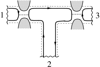
Figure 2: Partition noise geometry with two quantum point contacts. The correlation between contacts $2$ and $3$ is measured. The left most quantum point contact permits to control the population of the edge state.

The above consideration applies only to single particles. Statistical effects are a consequence of identical indistinguishable particles. Thus an approach to noise is necessary which takes the basic symmetries of many particle wave functions into account. In second quantization a general formulation of the noise power for non-interacting particles in terms of the scattering matrix $s_{\alpha\beta}$ was given in Refs. [5, 18, 24]. The scattering matrix $s_{\alpha\beta}$ relates current amplitudes incident in contact $\beta$ to out-going current amplitudes in contact $\alpha$. In the zero-temperature limit the current-correlations of interest are determined by a matrix

$$B_{\gamma\delta}=\sum_{\alpha}s_{\gamma\alpha}s^{\dagger}_{\delta\alpha}(f_{\alpha}-f_{0}),$$ (4)

where $f_{0}$ is an arbitrary energy dependent function. In terms of this matrix we find the cross-correlations ${\gamma\neq\delta}$,

$$S_{\gamma\delta}=-2(e^{2}/h)\int dETr[B^{\dagger}_{\gamma\delta}B_{\gamma\delta}].$$ (5)

This proofs that cross-correlations for Fermions are negative for conductors in zero-impedance external circuits [24, 18]. Would we repeat the calculation for photons emitted by black-body radiators [18] we would find that bunching of photons permits positive correlations. In what follows we use this expression to evaluate the cross-correlations.

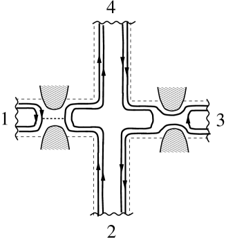
Figure 3: Partition noise geometry with two quantum point contacts. The inner edge state is completely reflected at both QPC’s. A dephasing voltage probe (contact $4$) generates noise even if also the outer edge state is perfectly transmitted at both QPC’s. An inelastic voltage probe (contact $4$) converts the shot noise generated at the left QPC into a positive current-correlation $S_{23}$.

4 Partition noise experiments

Consider the geometry of a conductor with two QPC’s in series as shown in Fig. 2, studied in the experiment of Oberholzer et al. [10]. The experiment measured the correlation $S_{23}$. Contact 1 is at a potential $eV$ and contacts 2 and 3 are grounded. The left and right QPC’s ($i=1$ and $i=2$) are described by scattering matrices

$$\left(\begin{array}[]{cc}\sqrt{R_{i}}&\sqrt{T_{i}}\\ -\sqrt{T_{i}}&\sqrt{R_{i}}\end{array}\right).$$ (6)

The resulting zero-temperature correlation function is

$$S_{23}=-2(e^{2}/h)|eV|T_{1}^{2}T_{2}R_{2}.$$ (7)

The transmission probability $T_{1}$ takes the role of the Fermi function: for $T_{1}=1$ the edge state is fully filled (degenerate), as $T_{1}$ becomes very small the edge state is only sparsely populated. In this latter limit classical Maxwell-Boltzmann statistics applies and the correlation function vanishes.

5 Effect of dephasing and inelastic scattering

Texier and one of us [25] investigated the effect of elastic (interedge state) scattering, of dephasing and of inelastic transitions on the correlation function given by Eq. (7). Inelastic scattering and dephasing can be investigated with the help of an additional contact, shown in Fig. 3. A real voltage probe acts as an inelastic scatterer. The electrochemical potential $\mu_{4}$ fluctuates as a function of time to maintain the total current into the probe at zero. In contrast a dephasing contact [26, 27] preserves the energies of the carriers at the contact: it is required that the current into the dephasing contact vanishes at each energy.

Figure 4: Optical Mach-Zehnder interferometer

For the single edge state used in the experiment by Oberholzer et al. it turns out that the correlation Eq. (7) is neither sensitive to elastic nor inelastic scattering. But the question becomes interesting if as shown in Fig. 3 there are two edge states.

The most interesting feature of the dephasing contact arises if both QPC’s transmit the outermost edge perfectly $T_{1}=T_{2}=1$ and reflect the innermost edge perfectly. If the dephasing probe is closed, the corresponding completely quantum coherent sample is noiseless. If we now switch on the dephasing voltage probe and allow as shown in Fig. 3 both edge channels to enter, the dephasing voltage probe generates noise!! The distribution function $\bar{f}_{4}(E)$ in the dephasing voltage probe, under the biasing condition considered here, is still a non-equilibrium distribution function and given by $\bar{f}_{4}(E)=\frac{1}{2}f_{1}(E)+\frac{1}{2}f_{2}(E)$. The distribution function at the dephasing contact is similar to a distribution at an elevated temperature with $kT=|eV|/4$ with $eV$ the voltage applied between contact $1$ and contacts $2$ and $3$. We have $\int dE\bar{f}_{4}(E)(1-\bar{f}_{4}(E))=e|V|/4$. Evaluation of the correlation function gives [25],

$$S^{\rm qe}_{23}=-({e^{2}}/{h})|eV|({1}/{4}).$$ (8)

The electron current incident into the voltage probe from contact $1$ is noiseless. Similarly, the hole current that is in the same energy range incident from contact $2$ is noiseless. However, the voltage probe has two available out-going channels. The noise generated by the voltage probe is thus a consequence of the partitioning of incoming electrons and holes into the two out-going channels. In contrast, at zero-temperature, the partition noise in a coherent conductor is a purely quantum mechanical effect. Here the partitioning invokes no quantum coherence and is a classical effect [28].

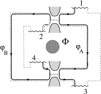
Figure 5: Edge state equivalent of the optical Mach-Zehnder interferometer. An Aharonov-Bohm fux penetrates the hole of the structure.

The interesting effect in the presence of a real voltage probe arises from the fact that the voltage in contact $4$ must fluctuate to maintain the current at zero. Here we now permit the left contact to have transmission probability $T_{1}\leq 1$. The resulting fluctuating voltage leads to the possibility of correlated injection of carriers into the two edge channels leaving the voltage probe. As a consequence the correlation function can now become positive even in a purely normal conductor. For the geometry of Fig. 3 we find [25],

$$S^{\rm in}_{23}=+({e^{2}}/{h})|eV|({1}/{2})T_{1}R_{1}.$$ (9)

This simple example shows that interactions can play an important role and lead to surprising results. Other related problems which show such a sign reversal include tunneling into a Luttinger liquid [29], dynamical spin-blockade in a ferro-magnetic-lead normal-dot system [30], or hybrid systems with superconductors, or frequency dependent transport [28].

Figure 6: Two-source, four-detector optical Hanbury Brown Twiss geometry. $\Phi$ represents an Aharonov-Bohm flux. After Ref. [8].

6 Mach-Zehnder geometry

The optical Mach-Zehnder geometry is shown in Fig. 4. The central property of a Mach-Zehnder geometry is that carriers (photons) exhibit only forward scattering. This is in contrast with the typical ring like structures used in mesoscopic physics where connection of a lead to a ring generates invariably backscattering and closed orbits. In principle, however, even in zero magnetic field a Mach-Zehnder interferometer can be realized with the help of X-junctions (see Ref. [31]). In high magnetic fields, with the help of edge states, a Mach-Zehnder interferometer has recently been realized by Ji et al. [32] and used to investigate the effect of decoherence on the shot noise [32, 33]. The structure is schematically shown in Fig. 5. A Corbino like geometry is used with two QPC’s. An electron incident from contact 1 is at the first QPC either transmitted or reflected. The transmitted partial wave proceeds along the outer edge to the second QPC whereas the reflected partial wave proceeds via the inner edge to the second QPC.

To be specific we choose the scattering matrix of the QPC to be given by Eq. (6). To simplify the results we take $T=R=1/2$. The interference of the partial waves in the exiting channel (second-order interference) leads to scattering matrix elements which are functions of both phases $\phi_{A}$ and $\phi_{B}$. For instance

$$s_{31}=(1/2)[\exp(i(\phi_{B}-\psi_{2}))+\exp(i(\phi_{A}+\psi_{1}))]$$ (10)

Here we have in addition to the geometric phases $\phi_{A}$ and $\phi_{B}$ added the effect of an Aharonov-Bohm flux through the center of the interferometer, $\psi_{1}+\psi_{2}=2\pi\Phi/\Phi_{0}$ with $\Phi_{0}=h/e$ the elementary flux quantum.

If contact $1$ is at an elevated potential $eV$ and all other contacts are grounded the current at contact $3$ is determined by the conductance $G_{31}=-(e^{2}/h)T_{31}$ which is

$$G_{31}=-(e^{2}/2h)(1+\cos(\phi_{B}-\phi_{A}-2\pi\Phi/\Phi_{0}))$$ (11)

The phase-dependence of the transmission and conductance is a consequence of the superposition of partial waves in an out-going channel. Our goal is now to show that there are geometries in which interference effects can arise in correlations even so all conductance matrix elements are phase-insensitive.

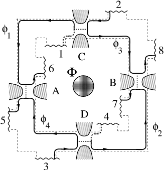
Figure 7: Two-source, four detector electrical Hanbury Brown Twiss geometry. After Ref. [8].

7 Exchange interference in HBT experiments

An optical two-source configuration [34] is shown in Fig. 6. It is equivalent to the stellar interferometer experiment of HBT. Two sources $2$ and $3$ illuminate detectors at contacts $5$ to $8$. Note that in this geometry there is no interference due to splitting of an incident wave and superposition of the resulting partial waves in an outgoing channel as in the Mach-Zehnder interferometer. Sources $2$ and $3$ are incoherent and their intensities at a detector add classically. Nevertheless the intensity-intensity correlations at contact pairs $58,57,68$ or $67$ are functions of the phases $\phi_{1}$ to $\phi_{4}$ as we will now show.

The electrical edge state equivalent [8] of the optical geometry of Fig. 6 is shown in Fig. 7. The elements of the scattering matrix now contain phases only in a trivial multiplicative way. For instance the scattering matrix element for transmission from source contact $2$ to the detector contact $5$ is

$$s_{52}=T_{A}^{1/2}\exp(i\phi_{1})T_{C}^{1/2}$$ (12)

Here $T_{C}$ and $T_{A}$ are the transmission amplitudes of the QPC’s denoted $C$ and $A$ in Fig. 7. Similar expressions hold for all other elements of the s-matrix. In contrast to the Mach-Zehnder interferometer here phase factors like $\exp(i\phi_{1})$ simply multiply the scattering matrix elements. An Aharonov-Bohm (AB) flux through the hole of this Corbino geometry similarly introduces only multiplicative phase factors. Consequently the conductance matrix is a function of the transmission and reflection probabilities of the individual QPC’s only.

To be definite let us take the transmission and reflection probabilities at the QPC denoted $C$ to be $T_{C}=T$ and $R_{C}=R$ and at $D$ to be $T_{D}=R$ and $R_{D}=T$. If the source contacts $2$ and $3$ are at a potential $eV$ and all other contacts are grounded the currents at the detector contacts are [8]

$$I_{5}=I_{6}=({2e^{2}}/{h})TV,\hskip 14.22636ptI_{7}=I_{8}=({2e^{2}}/{h})RV$$ (13)

independent of the transmission amplitudes of the QPC’s denoted by $A$ and $B$ in Fig. 7. Most importantly, the corresponding conductances reveal no phase dependence and are independent of the AB-flux $\Phi$.

In contrast to the conductance matrix the correlation functions now depend on the phases. Consider the simple case where transmission and reflection amplitudes of all QPC’s are equal to $1/2$. The correlation function $S_{58}$ is [8]

$$S_{58} = -(e^{2}/4h)|eV|$$ (14)

$$\times (1+\cos(\phi_{1}+\phi_{2}-\phi_{3}-\phi_{4})).$$

The correlation function thus depends in an essential way on the phases accumulated by different particles from the source contact to the detector contact. An AB-flux through the hole of the Corbino disk contributes a positive phase to $\phi_{1}$ and $\phi_{2}$ and a negative phase to $\phi_{3}$ and $\phi_{4}$ to give a total additional phase contribution of $2\pi\Phi/\Phi_{0}$. Thus we have a geometry for which conductances exhibit no AB-effect but correlation functions are sensitive to the variation of an AB-flux!

The two particle Aharonov-Bohm effect demonstrates nicely that quantum interference is not simply related to properties of single particle states. The existence of such an additional phase-sensitivity of forth-order interference was recognized in early work on noise correlations: An early paper [24] on noise in multi-terminal mesoscopic conductors was entitled ”The quantum phase of flux correlations in wave guides”. However, neither in this work nor in subsequent efforts [35, 36, 37] was a geometry found in which the effect can be seen in such a clear cut way as in the geometry of Fig. 7. The first term in Eq. (14) is the sum of the correlations that are obtained if only source $2$ is active and if only source $3$ is active. These single source correlations are phase-insensitive. Indeed in the presence of complete dephasing (described e.g. with the help of an energy conserving voltage probe, say at the outer edge between QPC’s $C$ and $A$) it is precisely the first term in Eq. 14 which survives [38].

In optics, set-ups with independent sources similar to Fig. 6 have been proposed theoretically [34] and investigated experimentally [40] in the context of entanglement and Bell Inequalities(BI). However, non-thermal sources and coincidence measurements have been employed. Neither of these are available in electrical conductors. Nevertheless, the joint photon detection probabilities [41] used to test BI, have the same phase dependence as the correlation function Eq. (14). This naturally raises the question if the above correlations are not also in fact a consequence of entanglement of the carriers emitted by the two reservoirs? Moreover, if this is the case, can this entanglement be used to violate a BI expressed in terms of the zero-frequency correlators? Below, we show that the answer to both these questions is yes.

8 Entanglement and HBT experiments

Instead of modulating the phases in Eq. (14) via the path lengths, we investigate the correlation functions in the two-source HBT set-up of Fig. 7 by varying the transmission through the two QPC’s $A$ and $B$ which precedes the detector contacts. This is similar to schemes in optics where one varies the transmission to the detectors with the help of polarizers. The advantage of this latter approach is that the Bell Inequalities in the presence of dephasing [42] (in general not a problem in optics) can be violated over a wider range of parameters [43].

Detection of entanglement via violation of a Bell Inequality (BI) in electrical conductors is discussed in Refs. [44, 45, 42, 46, 47, 48]. Following the original suggestion of Bohm and Aharonov[49], it is most tempting to treat spin entanglement. However, it is charge current fluctuations that are measured and the conversion of spin to charge information adds to experimental complexity. Entanglement can, however, take other forms [42, 46, 48] and below we follow Refs. [42, 46] and discuss entanglement of orbital degrees of freedom.

To simplify the following discussion we now assume an AB-flux $\Phi$ such that the phases in Eq. (14) add up to a multiple of $2\pi$. The transmission and reflection probabilities through the detector QPC’s are taken to be $T_{A}=1-R_{A}=\sin^{2}(\theta_{A})$ for $A$ and with $\theta_{A}$ replaced by $\theta_{B}$ for $B$). Ref. [8] finds the noise powers

$$S_{58}=S_{67}=-({2e^{2}}/{h})|eV|RT\cos^{2}(\theta_{A}-\theta_{B}),$$ (15)

$$S_{57}=S_{68}=-({2e^{2}}/{h})|eV|RT\sin^{2}(\theta_{A}-\theta_{B}).$$ (16)

The non-local dependence on the angles $\theta_{A}$ and $\theta_{B}$ is just the one found for the two-particle joint detection probability in the context of two-particle entanglement, as originally discussed by Bell [41].

To provide a clear picture of entanglement in the HBT geometry we now explicitly construct the many-body state generated by the two incoherent source reservoirs $2$ and $3$. In a second quantization notation (suppressing the spin index) the transport state generated by the two sources is

$$|\Psi\rangle=\prod_{0<E<eV}c_{2}^{\dagger}(E)c_{3}^{\dagger}(E)|0\rangle$$ (17)

where $|0\rangle$ is the ground state, a filled Fermi sea in all reservoirs at energies $E<0$. The operator $c^{\dagger}_{\alpha}(E)$ creates an injected electron from reservoir $\alpha$ at energy $E$. To analyze this state consider first a pair of single electrons at energy $E$ described by $c_{2}^{\dagger}c_{3}^{\dagger}|0\rangle$. Let us denote the creation operators of particles reflected at $C$ by $c_{2B}^{\dagger}$ and of particles transmitted at $C$ by $c_{2A}^{\dagger}$. Similarly, let us denote the creation operators of particles reflected at $D$ by $c_{3A}^{\dagger}$ and of particles transmitted by $c_{3B}^{\dagger}$. The second index $A,B$ thus denotes towards which beam-splitter the electron is propagating. The state (keeping in mind that $C$ transmits with probability $T$ and $D$ transmits with probability $R$) beyond the QPC’s C and D is then [8]

$$|\Psi\rangle=|\tilde{\Psi}\rangle+|\Psi_{T}\rangle+|\Psi_{R}\rangle$$ (18)

with

$$|\tilde{\Psi}\,\,\,\rangle = \sqrt{RT}\left(c_{2A}^{\dagger}c_{3B}^{\dagger}+c_{2B}^{\dagger}c_{3A}^{\dagger}\right)|0\rangle$$

$$|\Psi_{T}\rangle = Tc_{2A}^{\dagger}c_{3A}^{\dagger}|0\rangle,|\Psi_{R}\rangle=Rc_{2B}^{\dagger}c_{3B}^{\dagger}|0\rangle$$ (19)

The total state $|\Psi\rangle$ consists of a contribution, $|\tilde{\Psi}\rangle$, in which the two particles fly off one to $A$ and one to $B$, and of two contributions, $|\Psi_{R}\rangle$ and $|\Psi_{T}\rangle$, in which the two particles fly both of towards the same detector contact.

A particularly simple limit is the case of strong asymmetry $R\ll 1$, where almost all electrons are passing through both source beam splitters towards detector $A$. In this limit, the state $|\Psi_{R}\rangle$ can be neglected. Moreover, by redefining the vacuum to be the completely filled stream of electrons, i.e. introducing $|\bar{0}\rangle=c_{2A}^{\dagger}c_{3A}^{\dagger}|0\rangle$, we can write the state $|\Psi\rangle$ to leading order in $\sqrt{R}$ as

$$|\Psi\rangle=\left(1+\sqrt{R}\left[c_{3B}^{\dagger}c_{3A}-c_{2B}^{\dagger}c_{2A}\right]\right)|\bar{0}\rangle$$ (20)

The operators $c_{3A}(E)$ and $c_{2A}(E)$ now describe hole excitations, i.e. the removal of electrons from the filled stream. To leading order in $\sqrt{R}$ the total state in Eq. (17), including again the full energy dependence, can thus be written as

$$|\Psi\rangle =|\bar{0}\rangle+$$ (21)

$$\sqrt{R} \int_{0}^{eV}dE\left[c_{3B}^{\dagger}(E)c_{3A}(E)-c_{2B}^{\dagger}(E)c_{2A}(E)\right]|\bar{0}\rangle$$

Due to the redefinition of the vacuum [42], we can interpret the resulting state as describing a superposition of electron-hole pair excitations out of the ground state (created at C and D), i.e. an orbitally entangled pair of electron-hole excitations. This is equivalent to the recent findings by Beenakker et al, [46], who discussed the generation of entangled electron-hole pairs at a single QPC. The state is similar to the two-electron state considered by Samuelsson, Sukhorukov and Büttiker, [42], emitted from a superconductor contacted at two different points in space. We note that that the new vacuum $|\bar{0}\rangle$ does not contribute to the current correlators since it describes a filled, noiseless stream of electrons.

Can we formulate a BI in terms of the zero-frequency cross-correlators Eq. (16)? In the strongly asymmetric case, $R\ll 1$, this is clearly the case. The state in Eq. (21), describes Poissonian emission of orbitally entangled electron-hole pair wave packets. Following Ref. [42], the average time between each emission is much longer than the coherence time of each pair, and the zero frequency cross correlations are just identical to a coincidence measurement, running over a long time. The electron-hole joint detection probability is proportional to the zero frequency cross correlations. One can then apply the arguments in the original paper of Bell [41] and directly formulate a BI in terms of the zero frequency cross correlators [42] for four different angle configurations $-2\leq S_{B}\leq 2$, in the form [50, 51]

$$S_{B}=E(\theta_{A},\theta_{B})-E(\theta_{A},\theta_{B}^{\prime})+E(\theta_{A}^{\prime},\theta_{B})+E(\theta_{A}^{\prime},\theta_{B}^{\prime})$$ (22)

where the Bell correlation functions

$$E(\theta_{A},\theta_{B})={\left(S_{58}+S_{67}-S_{57}-S_{68}\right)}/S_{0}$$ (23)

with $S_{0}=-{(4e^{2}RT/h)}|eV|$ are given by

$$E(\theta_{A},\theta_{B})=\cos(2[\theta_{A}-\theta_{B}]).$$ (24)

By adjusting the four angles the maximal Bell parameter is $S=2\sqrt{2}$ and the BI is thus violated.

We note that the phase dependence of the current correlators in Eq. (16) is not a result from taking the limit $R\ll 1$. However, for $R$ not small, many electron-hole pairs are superimposed on each other during the measurement, i.e. the average emission time of the electron-hole pairs is of the order of the pair-coherence time. As pointed out above, the derivation of the BI in Eq. (22) rest on the assumption that the pairs are well separated, and the BI can thus not be applied for arbitrary $R$. Whether the phase dependence of the correlators in Eq. (16) results from some kind of multiparticle entanglement and whether this entanglement can be detected via a violation of a BI, are interesting questions which however go beyond the scope of the present paper.

We have discussed only the case of integer quantum Hall states. The fractional quantum Hall effect offers a wider, very interesting, area for the examination of correlations [52, 53] since in this case fractional statistical effects are realized.

The HBT effect and the BI both concern two particle effects. In this work we have established a relation between the two. The simple adiabatic edge-state geometry described above using only normal reservoirs as particle sources, the focus on orbital non-locality and the use of zero-frequency correlators brings experimental detection of entanglement in electrical conductors within reach.

Note added in proof

Since submission of this work, we have included a treatment in Ref. [8] of entanglement and violation of a Bell Inequality due to post-selection for a nearly symmetric (large transmission interferometer) going beyond the tunneling limit. We acknowledge discussion and correspondence (unpublished) with C. W. J. Beenakker on this topic.

References

- [1] K. von Klitzing, G. Dorda, M. Pepper, Phys. Rev. Let. 45 (1980) 494.
- [2] B. J. van Wees, et al. Phys. Rev. Lett. 60 (1988) 848.
- [3] D. A. Wharam et al. J. Phys. C21 (1988) L861.
- [4] G. Müller et al. Phys. Rev. B42 (1990) 7633.
- [5] M. Büttiker, Phys. Rev. Lett. 65 (1990) 2901.
- [6] R. Hanbury Brown, R.Q. Twiss, Nature 178 (1956) 1046.
- [7] E.M. Purcell, Nature 178 (1956) 1449
- [8] P. Samuelsson, E. Sukhorukov, M. Büttiker, (unpublished). cond-mat/0307473
- [9] M. Henny et al, Science 284 (1999) 296.
- [10] S. Oberholzer et al., Physica 6E, (2000) 314.
- [11] W.D. Oliver et al. Science 284 (1999) 299.
- [12] H. Kiesel et al, Nature 418 (2002) 392.
- [13] B. J. Halperin, Phys. Rev. B25 (1982) 2185
- [14] M. Büttiker, Phys. Rev. B38 (1988) 9375
- [15] B. J. van Wees et al. Phys. Rev. B 39 (1989) 8066; S. Komiyama et al. Solid State Commun. 73 (1990) 91; B. W. Alphenaar et al. Phys. Rev. Lett. 64 (1990) 677.
- [16] For reviews see: M. Büttiker, in ”Nanostructured Systems”, edited by Mark Reed, Semiconductor and Semimetals, Vol. 35, Academic Press, Boston, MA, 1991, p. 191; R. J. Haug, Semicond. Science and Technol. 8 (1993) 131.
- [17] T. Christen, M. Büttiker, Phys. Rev. B53 (1996) 2064; S. Komiyama and H. Hirai, Phys. Rev. B 54 (1996) 2067.
- [18] M. Büttiker, Phys. Rev. B 46 (1992) 12485.
- [19] Ya. M. Blanter, M. Büttiker, Phys. Rep. 336 (200) 1.
- [20] V. A. Khlus, Zh. Éksp. Teor. Fiz. 93 (1987) 2179 [Sov. Phys. JETP 66 (1987) 1243].
- [21] G. B. Lesovik, Pis’ma Zh. Éksp. Teor. Fiz. 49 (1989) 513 [JETP Lett. 49 (1989) 592].
- [22] T. Martin, R. Landauer, Phys. Rev. B 45 (1992) 1742.
- [23] M. I. Reznikov, et al., Phys. Rev. Lett. 75 (1995) 3340; A. Kumar, et al., Phys. Rev. Lett. 76 (1996) 2778 (1996).
- [24] M. Büttiker, Physica B175 (1991) 199.
- [25] C. Texier, M. Büttiker, Phys. Rev. B 62 (2000) 7454.
- [26] M. J. M. de Jong, C. W. J. Beenakker, Physica A 230, (1996) 219.
- [27] S.A. van Langen, M. Büttiker, Phys. Rev. B 56 (1997) 1680.
- [28] M. Büttiker, in Quantum Noise in Mesoscopic Physics, edited by Yu. Nazarov, (Kluwer Academic Publishers, Netherlands, 2003). p. 3.
- [29] A. Cr pieux et al., Phys. Rev. B 67, (2003) 205408.
- [30] A. Cottet, W. Belzig and C. Bruder, unpublished, cond-mat/0308564.
- [31] G. Seelig, M. Buttiker, Phys. Rev. B 64 (2001) 245313; G. Seelig, et al., cond-mat/0304022
- [32] Y. Ji et al., Nature 422 (2003) 415.
- [33] F. Marquardt, C. Bruder, cond-mat/0306504
- [34] B. Yurke, D. Stoler, Phys. Rev. A 46 (1992) 2229.
- [35] M. Büttiker, Phys. Rev. Lett. 68 (1992) 843.
- [36] T. Gramespacher, M. Buttiker, Phys. Rev. Lett. 81 (1998) 2763; Phys. Rev. B60 (1999) 2375.
- [37] D. Loss, E. V. Sukhorukov, Phys. Rev. Lett. 84 (2000) 1035.
- [38] A related question is the robustness of exchange interference effects under ensemble averaging. It is shown Refs. [27, 19, 39] that even if the contributions to the correlation from single sources are subtracted ensemble averaging gives a finite result.
- [39] E. V. Sukhorukov, D. Loss, Phys. Rev. B 59 (1999) 13054.
- [40] See B. Pittman and J.D. Franson, Phys. Rev. Lett. 90 (2003) 240401 and refs. therein.
- [41] J. Bell, Physics 1 (1964) 195.
- [42] P. Samuelsson, E. Sukhorukov, M. Büttiker, Phys. Rev. Lett., unpublished, cond-mat/0303531.
- [43] The single edge state geometry discussed here is especially robust against dephasing. See P. Samuelsson, E. Sukhorukov, and M. Büttiker, Special issue on ”Quantum Computation at the Atomic Scale”, Turkish Journal of Physics, cond-mat/0309540. In the presence of two or more edge states, interedge state scattering makes it more difficult to observe violations of a Bell inequality. See J.L. van Velsen, M. Kindermann, C.W.J. Beenakker, Special issue on ”Quantum Computation at the Atomic Scale”, Turkish Journal of Physics, unpublished, cond-mat/0307198.
- [44] X. Maître, W. D. Oliver, Y. Yamamoto, Physica E 6 (2000) 301; S. Kawabata, J. Phys. Soc. Jpn. 70 (2001) 1210.
- [45] N. M. Chtchelkatchev, et al., Phys. Rev. B 66 (2002) 161320.
- [46] C.W.J. Beenakker et al. Phys. Rev. Lett., unpublished, cond-mat/0305110
- [47] L. Faoro, F. Taddei, R. Fazio, cond-mat/0306733
- [48] V. Scarani, N. Gisin, S. Popescu, (unpublished). cond-mat/0307385
- [49] D. Bohm and A. Aharonov, Phys. Rev. 108 (1957) 1070.
- [50] J. F. Clauser et al, Phys. Rev. Lett. 23 (1969) 880.
- [51] A. Aspect, P. Grangier, and G. Roger, Phys. Rev. Lett 49 91, (1982).
- [52] I. Safi, P. Devillard, T. Martin, Phys. Rev. Lett. 86 (2001) 4628.
- [53] S. Vishveshwara, (unpublished). cond-mat/0304568