Regular and Singular Fermi Liquid Fixed Points in Quantum Impurity Models

Abstract

We show that thermodynamics is insufficient to probe the nature of the low energy dynamics of quantum impurity models and a more subtle analysis based on scattering theory is required. Traditionally, quantum impurity models are classified into one of two categories: Fermi liquids and non-Fermi liquids, depending on the analytic properties of the various thermodynamic quntities. We show, however, that even when a quantum impurity model is a Fermi liquid (an incoming electron at the Fermi level scatters elastically off the impurity), one may find singular thermodynamic behavior if characteristics of quasiparticles are not analytic near the Fermi surface. Prompted by this observation, we divide Fermi liquids into two categories: regular Fermi liquids and singular Fermi Liquids. The difference between regular Fermi liquids, singular Fermi liquids , and non-Fermi liquids fixed points is explained using properties of the many-body $S$-matrix for impurity quasiparticle scattering. Using the Bethe-Ansatz and numerical RG, we show that whereas the ordinary Kondo Model is a regular Fermi liquid the underscreened Kondo model is a a singular Fermi liquid. This results in a breakdown of Nozières’ Fermi liquid picture for the underscreened and explains the singular thermodynamic behavior noticed in Bethe Ansatz and large-$N$ calculations. Furthermore, we show that conventional regular Fermi liquid behavior is re-established in an external magnetic field $H$, but with a density of states which diverges as $1/H$. Possible connections with the field-tuned quantum criticality recently observed in heavy electron materials are also discussed.

I Introduction

Quantum impurity models have been studied extensively in condensed matter physics both experimentally and theoretically. Many approaches have been developed to characterize their low energy physics. Conventionally, systems are classified into one of two categories, Fermi liquid (FL)noz and non-Fermi Liquid (NFL) depending on their low temperature specific heat behavior. In particular, systems with non-integer power dependence on temperature are called NFLs. In this paper, we show that thermodynamics is insufficient to probe the nature of the low energy dynamics and a more subtle analysis based on electron-impurity scattering theory is required. We illustrate our ideas using recent as well as established results on the underscreened Kondo Model (UKM).

In a Fermi liquid, the low energy dynamics are described in terms of well defined quasi-particles close to a Fermi-surface. Furthermore, for an impurity problem, the quasiparticles at the Fermi energy are isomorphic to the original electron states. For this reason, electrons at the Fermi energy scatter elastically off the impurity: both the ingoing and outgoing states consist of a single electron. However, in a generic non-Fermi liquid impurity system, this is not the case. Even when the incoming electrons are on the Fermi surface they can scatter inelastically; an incoming electron state does not scatter into a single outgoing electron state, but instead, excites a large variety of collective modes including particle-hole excitations. For example, in the extreme case of the two-channel Kondo model, the out going scattering state does not include any single electron component after scattering with the impurity Ludwig .

This difference between Fermi liquids and non-Fermi liquids manifests itself most clearly in the renormalization group (RG) flow of the single particle matrix elements of the many-body $S$-matrix, $\langle k\;\mu,{\rm in}|\hat{S}|k^{\prime}\;\mu^{\prime},{\rm in}\rangle$ where $k$ and $k^{\prime}$ denote the momenta of incoming and outgoing electrons and $\mu,\mu^{\prime}$ the rest of their quantum numbers. In the space of single electrons states it is easy to show (see below) that the matrix elements depend only on $\omega=k=k^{\prime}$ where $\omega$ denotes the energy of incoming particle measured with respect the the Fermi energy. Unitarity requires $S(\omega)$ to be a complex number with modulus less than equal to one. Using RG one obtains the behavior of the theory at $\omega=0$. For a Fermi liquid $|S(\omega=0)|=1$ implying that at the Fermi level, the inelastic scattering cross section vanishes and single particle at the scattering is completely characterized by a phase shift. On the other hand, for a non-Fermi liquid model, $|S(\omega=0)|<1$. Consequently, NFLs have a non-vanishing many particle scattering rate and a finite inelastic scattering cross section at the Fermi surface.

We shall argue below that even when a quantum impurity is a Fermi-liquid in the sense described above one may still find singular thermodynamic behavior. This occurs when characteristics of quasiparticle are not analytic near the Fermi surface. In terms of scattering, this means that the eigenvalues of the S-matrix for impurity quasi-particle scattering approach the unit circle non-analytically as the quasi-particle energy $\omega$ approaches the Fermi level. For this reason, it is necessary to divide Fermi liquids into two types: regular Fermi liquids (RFL) and singular Fermi liquids (SFL). In the former, the eigenvalues of the single particle S-matrix approach the unit circle analytically whereas in the latter, they approach it singularly. For both types of fixed points, the single particle $S$-matrix is unitary and an incoming electron at the Fermi surface scatter elastically off the impurity. However, the two types of FLs exhibit very different phenomenological properties. A regular Fermi liquid exhibits the usual properties associated with FLs, and hence, by an abuse of notation, we shall often omit the term ‘regular’ when referring to this class of fixed points. On the other hand, SFLs exhibit a wide variety of behavior not ordinarily associated with Fermi liquids such as extreme sensitivity to applied fields and a divergent specific heat.This classification scheme and the main properties of the three impurity classes are summarized in Fig. 1.

An example of the difference between regular and singular FLs is seen in the striking difference in the strong coupling physics of the ordinary Kondo Model (KM) and the underscreened Kondo Model (UKM) (see  varkondo and references within). The UKM describes the interaction of a magnetic impurity with spin $S>1/2$ with a sea of conduction electrons. In the UKM, the impurity and the electrons are coupled by anti-ferromagnetic interaction. At low temperatures, the impurity spin is therefore partially screened from spin S to spin $S^{*}=S-1/2$. What distinguishes the UKM from the ordinary Kondo model is the residual magnetic moment that remains even after screening. This residual moment couples ferromagnetically to the remaining conduction electrons. Though the ferromagnetic coupling is irrelevant, it tends to zero very slowly. As a result, there is a subtle interplay between the residual moment and the electron fluid that leads to radically different physics from the ordinary KM at the strong-coupling fixed point of the UKM.

A Bethe-Ansatz and a large $N$ analysis of the underscreened Kondo model revealed that at zero field, this system exhibits singular behavior, with a divergent specific heat coefficient $C_{v}/T$ at zero field sacramento ; CPe . In a finite field, the linear specific heat coefficient was found to diverge as $1/(B\;{\rm ln}^{2}(T_{K}/B)$. To study the scattering properties of the model we re-examine it using the Bethe-Ansatz and the numerical renormalization group (NRG). From the Bethe-Ansatz solution, we find that the sacttering matrix and density of states of spinons at the impurity (DOS) is a singular function of quasi-particle energy in zero magnetic field. The DOS becomes analytic in finite fields; however, it shows a singular behavior as the magnetic field scales to zero. These results are confirmed using the numerical renormalization group (NRG) calculations, where we can directly compute the phase shift of spin 1/2 electron excitations from the finite size spectrum. The singular nature of the DOS results in the breakdown of Nozières’ picture of the strong coupling fixed point and indicates that the physics of the UKM and the ordinary Kondo model are quite different. However, despite this singular behavior,the NRG calculations confirm that the fixed point finite size spectrum of the UKM is that of a Fermi liquid, i.e., it can be characterized by a simple phase shift $\pi/2$.

The analysis we present here may also be relevant to heavy fermion systems. Over the years, much of new insight obtained in heavy electron physics has been acquired from the study of simplified, impurity models  4 . Anderson’s original model for the formation of local moments, is itself an impurity model. Doniach’s Kondo lattice scenario for heavy electron metals was based on an understanding of the impurity Kondo model, long before approximate solutions to the lattice were available  doniach . The idea to use a large $N$ expansion for the Kondo lattice model, grew from a corresponding study of single impurity models  largeN and early motivation for the understanding of non-Fermi liquid behavior in Uranium heavy fermion systems grew from an application of the two-channel Kondo model to these systems  cox . Most recently, impurity models have played a role in proposed models for the quantum critical behavior of heavy electron systems  qcp .

In recent experimental studies, heavy electron materials were fine-tuned away from an antiferromagnetic quantum critical point (QCP) using a magnetic fieldgegenwart ; Custers , revealed that parameters of the heavy Fermi liquid can be field-tuned. In particular, the temperature dependent properties of the system near the QCP were shown to depend only on the ratio $T/(B-B_{c})$. Therefore one can draw parallels with the field tuned change in behavior of the UKM from a SFL to a regular FL.

Figure 1: Sketch of the renormalization group flows of the eigenvalues of the single particle $S$-matrix. The eigenvalues are within the unit circle. Particles at high enough energies ($\omega\to\infty$) do not see the impurity, therefore $S\to 0$ in this limit. Inelastic scattering processes are allowed whenever $|S(\omega)|<1$. In Fermi liquids at the Fermi energy $|S(\omega=0)|=1$, implying the absence of inelastic scattering of electrons. For non-Fermi liquids $|S(\omega=0)|<1$, while for singular Fermi liquids $S(\omega)$ approaches the unit circle non-analytically as $\omega\to 0$.

This paper is structured as follows. In Section 2, we discuss the general classification of regular and singular Fermi Liquids and the application of this classification scheme for Kondo models in more detail. In section 3, we use the Bethe-Ansatz to calculate the DOS and find that it is singular in the absence of a magnetic field. In Section 4, we present Numerical Renormalization Group calculations confirming our Bethe-Ansatz results. In Section 5, we discuss the breakdown of Nozières Fermi liquid picture for the UKM. Finally, we discuss connections with field-tuned criticality and some future lines of research. Some details of the Bethe Ansatz calculation are given in Appendix I.

II Singular Fermi Liquids and Non-Fermi Liquids

In a Fermi liquid impurity model the quasiparticle excitations at the Fermi level become identical to undressed conduction electrons. In other words, an incoming electron at the Fermi energy scatters into a single outgoing electron. In contrast, in a non-Fermi liquid impurity model, such as the two-channel Kondo model, quasiparticle excitations do exist, but are orthogonal to the original incoming electrons. This implies that in a non-Fermi liquid impurity model only a fraction of an incoming electron scatters into a single electron state, with the rest exciting particle-hole excitations via inelastic scattering. In the extreme case of the two-channel Kondo model, e.g., the outgoing state can be shown to be completely orthogonal to a single electron state.Maldacena ; JanZar

These properties can be most easily captured through the many body $S$-matrix, which we shall analyze in the rest of this section. The discussion of the $S$-matrix will allow us, in particular, to distinguish between non-Fermi liquid and singular Fermi liquid systems.

Let us consider a general quantum impurity problem at $T=0$ temperature, described by the following Hamiltonian

$$H=-i\sum_{\mu}\int dx\;:\psi_{\mu}^{\dagger}(x,t)\partial_{x}\psi_{\mu}(x,t):+H_{\rm int}\;.$$ (1)

Here the fields $\psi_{\mu}$ are chiral one-dimensional fermions, and usually represent radial excitations in some three-dimensional angular momentum channel coupled to the impurity. The label $\mu$ represents those discrete internal degrees of freedom (spin, flavor, crystal field, angular momentum indices, etc.) that may couple to the impurity. The precise form of the impurity-fermion interaction, $H_{\rm int}$ is of no importance for the purpose of our discussion below.

The central quantity we are interested in is the many-body $S$-matrix, $\hat{S}$, defined in terms of incoming and outgoing scattering states, $|a\rangle_{\rm in}$ and $|b\rangle_{\rm out}$ as (see e.g. Itzikson )

$$\langle b,{\rm out}|\;a,{\rm in}\rangle\equiv\;\langle b,{\rm in}|\hat{S}|\;a,{\rm in}\rangle\;.$$ (2)

The ’in’ and ’out’ states are eigenstates of the total Hamiltonian, Eq. (1), satisfying the boundary conditions that they tend to plane waves in the $t\to-\infty$ and $t\to\infty$ limits, respectively. In the interaction representation, the explicit form of the $S$-matrix is given by the well-known expression $\hat{S}={\rm T}\exp\{-i\int_{-\infty}^{\infty}H_{\rm int}(t)\;dt\}$, where ${\rm T}$ is the time ordering operator, and the interaction $H_{\rm int}(t)$ is adiabatically turned on and off during the time evolution. In the following, we shall only be interested in the single particle matrix elements of the $S$-matrix,

$$\langle k\;\mu,{\rm in}|\hat{S}|k^{\prime}\;\mu^{\prime},{\rm in}\rangle=2\pi\;\delta(k-k^{\prime})\;{\cal S}_{\mu\mu^{\prime}}(\omega)\;,$$ (3)

where $k$ and $k^{\prime}$ denote the momenta of incoming and outgoing electrons. In Eq. (3) we separated a Dirac delta contribution due to energy conservation and thus defined the on shell single particle $S$-matrix, $\cal S(\omega)_{\mu\mu^{\prime}}$, with $\omega=k$ the energy of the incoming and outgoing electrons Itzikson .

Unitarity of the $S$-matrix poses severe constraints on the eigenvalues $s_{\lambda}(\omega)\equiv r_{\lambda}(\omega)e^{i2\delta_{\lambda}(\omega)}$ of $\cal S$, which must be within the unit circle:

$$|s_{\lambda}(\omega)|=r_{\lambda}(\omega)\leq 1\;.$$ (4)

If $\cal S$ has an eigenvalue that is not on the unit circle, this implies that one can construct an incoming single particle state which with some probability scatters inelastically into a multi-particle outgoing state. To show this more explicitly, let us consider the $T$-matrix defined through

$$\hat{S}=\hat{1}+i\;\hat{T}\;.$$

We can then define the on-shell $T$-matrix ${\cal T}(\omega)_{\mu\mu^{\prime}}$ analogous to Eq. (3), and the corresponding eigenvalues are simply given by

$$\tau_{\lambda}(\omega)=-i\;(s_{\lambda}(\omega)-1)\;.$$ (5)

As discussed in Ref. dephasing, , the knowledge of the single particle matrix elements of the many-body $T$-matrix enables us to compute the total scattering cross section off the impurity in the original three-dimensional impurity problem through the optical theorem as

$$\sigma_{\rm tot}=\sigma_{0}\sum_{\lambda}2\;|\varphi_{\lambda}(\omega)|^{2}{\rm Im}\{\tau_{\lambda}(\omega)\}\;,$$ (6)

where $\sigma_{0}=\pi/k_{F}^{2}$ with $k_{F}$ the Fermi momentum, and $\varphi_{\lambda}(\omega)$ denotes the wave function amplitude of the incoming electron in scattering channel $\lambda$. Elastic scattering off the impurity can be defined as single particle scattering processes where the outgoing state consists of a single outgoing electron. The elastic scattering cross section is simply proportional to the square of the elements of the $T$-matrix, and is given by

$$\sigma_{\rm el}=\sigma_{0}\sum_{\lambda}|\varphi_{\lambda}(\omega)|^{2}|\tau_{\lambda}(\omega)|^{2}\;.$$ (7)

Having determined both $\sigma_{\rm tot}$ and $\sigma_{\rm el}$, we can define the inelastic scattering cross section off the impurity as the difference of these cross sections,JanZawa $\sigma_{\rm inel}=\sigma_{\rm tot}-\sigma_{\rm el}$,

$$\sigma_{\rm inel}=\sigma_{0}\sum_{\lambda}|\varphi_{\lambda}(\omega)|^{2}(1-r_{\lambda}(\omega)^{2})\;.$$ (8)

We define a quantum impurity model to be of non-Fermi liquid type if some of the eigenvalues of the single particle $S$-matrix are not on the unit circle in the $\omega\to 0$ limit. By Eq. (8) this immediately implies that non-Fermi liquid models have the unusual property that even electrons at the Fermi energy can scatter off the impurity inelastically with a finite probability.

Typical examples of non-Fermi liquid models are given by over-screened multichannel Kondo models. In the two channel Kondo model, e.g., it has been shown in Refs. Maldacena and  JanZar using bosonization methods that the single particle matrix elements of the S-matrix identically vanish at the Fermi energy, immediately implying that $r_{\lambda}=0$ and thus $\sigma_{\rm el}=\sigma_{\rm inel}=\sigma_{\rm tot}/2$ at the Fermi energy footnote ; dephasing .

Most other models, however, such as screened or under-screened Kondo models, the Anderson impurity model, the resonant level model, or over-screened models in an external field, fall in the category of Fermi liquids, since in all these cases all eigenvalues of the single particle $S$-matrix are located on the unit circle at $\omega=0$. This implies that in Fermi liquids electrons at the Fermi energy scatter completely elastically off the impurity, and that this scattering can be characterized in terms of simple phase shifts.

The structure of the energy dependence of the $s_{\lambda}(\omega)$’s, i.e. the renormalization group flow of the eigenvalues of the single particle $S$-matrix, however, does depend on the specific Fermi liquid model, and allow for further classification: We can define as singular Fermi liquids those models, where the convergence to the $\omega=0$ Fermi liquid fixed point is singular in $\omega$, while we shall call regular Fermi liquids those, where the convergence is analytical. By these terms, the standard spin 1/2 Kondo model is a regular Fermi liquid, while under-screened Kondo models such as the $S=1$ single channel Kondo model studied in this paper belong to the class of singular Fermi liquids. We shall see below that singular Fermi liquids have singularities in the low energy thermodynamic properties while having only elastic (albeit singular elastic) scattering on the Fermi surface.

The properties of the flows of the eigenvalues of the single particle scattering matrix $\cal S$ have been summarized for the three classes of quantum impurity models in Fig. 1.

External perturbations such as a magnetic field, e.g, can usually generate a cross-over to a regular Fermi liquid state in non-Fermi liquid or singular Fermi liquid models. However, the parameters of the resulting regular Fermi liquid may depend non-analytically on the external perturbations, and the corresponding Fermi liquid energy scale vanishes in the absence of them. Therefore the properties of these Fermi liquids become singular as a function of the external perturbation. The $S>1/2$ single channel Kondo model studied here, e.g., becomes a regular Fermi liquid in a magnetic field, however, the phase shifts $\delta_{s}(\omega=0)$ exhibit logarithmic singularity as a function of the magnetic field, corresponding to a divergent impurity DOS in the $H\to 0$ limit.

III Bethe Ansatz Calculation of the Density of States for the Underscreened Kondo Model

We proceed to show that the UKM is an example of a singular FL by analyzing the density of states, DOS, and the phase shift of electrons scattering off the impurity. We show that in zero magnetic field the DOS is a singular function of quasiparticle energy. We also show that while $|s(\omega)|\to 1$ as $\omega\to 0$ the limit is approached in a singular manner. Finally, we study the effect of a magnetic field and show that the singularity in the DOS is cut off by a finite field.

The Hamiltonian for the UKM can be mapped to the following one-dimensional Hamiltonian

$$H_{UKM}=-i\sum_{a}\int dx\,\psi_{a}^{\dagger}(x)\partial_{x}\psi_{a}(x)+J\left(\psi_{a}^{{\dagger}}(0)\vec{\sigma_{ab}}\psi_{b}(0)\right)\vec{S}\;,$$

where $\psi_{a}^{\dagger}(x)$ is the creation operator of an electron with spin $a$, and $\vec{S}$ is a localized spin at the origin coupled to the electron sea by an antiferromagnetic coupling $J$. In this equation the left-moving chiral Fermions $\psi_{a}^{\dagger}(x)$ in regions $x>0$ and $x<0$ simply represent the incoming and outgoing parts of the conduction electrons’ $s$ wave function in the three-dimensional problem.

The spectrum of the UKM can be determined from Bethe-Ansatz solution under ; wiegmann ; natan . The excitations consist of uncharged spin-1/2 excitations, spinons, and spinless charge excitations, holons. In the spinon-holon basis, the wavefunction for the electron can be written as a sum of products of a spin wavefunction and a charge wavefunction. Since the Kondo interaction affects only the spin sector, we will ignore the charge sector in the analysis that follows.

In the spin sector, an electron can be expressed as a superposition of spinons and anti-spinons. Formally, this is done through a form-factor expansion of the electron onto the spinon basis. At low-energies, the coefficients of the the multi-spinon terms in the form factor expansion tend to zero. For this reason, at sufficiently low energies, it is a reasonable to approximate the electron by a spinon natan82 . Since we are interested in the low-energy properties of the UKM, we will employ this approximation. The validity of this approximation will be checked by comparing our results at the Fermi energy with those of the Numerical Renormalization Group (NRG).

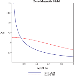
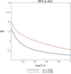
Figure 2: Fig.(a): The impurity induced (spinon) DOS of the $S=1/2$ Kondo model and the $S=1$ underscreened Kondo models as a function of the logarithm of the quasi-particle (spinon) energy. Figure (b): The same quantities in a finite magnetic field H. For $S=1/2$, the Impurity induced DOS is always finite. For the $S=1$ underscreened Kondo model, however, the DOS diverges in zero magnetic field as the energy of the excitation goes to zero. The presence of $H$ cuts off the singularity of the DOS of the underscreened Kondo model.

From the Bethe-Ansatz solution, we can calculate the phase shift $\delta_{s}(k,H)$ of a spinon with momentum $k$ when it is scattered off the impurity in the presence of a magnetic field $H$. The phase shift, in turn, is intimately related to the DOS of spinons at the impurity through the Friedel sum rule, which states that the spinon DOS, $N_{s}(\omega)$, is proportional to the derivative of the phase shift with respect to the energy  langreth . Note that as the energy of the spinon is linear in its momentum we shall use the symbols for momentum, $k$, and energy, $\omega$, interchageably (we have chosen units where $v_{F}=1$, so $\omega=k$.)

$$N_{s}(\omega,H)=\frac{1}{\pi}\frac{d\delta_{s}(\omega,H)}{d\omega}$$ (9)

To calculate the phase shift, we place our physical system in a finite ring of length $L$. The momentum $k$ of a free spinon will satisfy $k=\frac{2\pi}{L}n$, but in the presence of a impurity, by definition, the momentum will be shifted from its free value by twice the phase shift

$$k=\frac{2\pi}{L}n+\frac{2\delta_{s}(k=\omega,H)}{L}\;.$$ (10)

Since one can, using the Bethe-Ansatz solution, determine spinon momenta to accuracy $O(1/L)$, the phase shift can be exactly determined directly from the Bethe-Ansatz spectrum natan3 ; natan4 .

To solve for the spectrum of the UKM and to determine the phase shifts, it is necessary to solve a set of coupled integral-equations called the Bethe-Ansatz equations (BAE) footnote2 . The BAE are written in terms of the spin rapidities, $\Lambda$, and a spinon ’magnetic field’, $\Lambda_{B}$ (related to $H$, see later). Each set of $\{\Lambda\}$’s and $\Lambda_{B}$ which solve the BAE give rise to a set of physical momenta, $\{k\}$, and physical magnetic field $H$.

In the thermodynamic limit, instead of examining specific solutions of the BAE, it is sufficient to study the density of solutions. Let $\sigma(\Lambda)$ denote the density of solutions of the BAE in an interval $d\Lambda$ (not to be confused with the scattering cross section). A spinon excitation corresponds to removing a $\Lambda=\Lambda^{h}$ from the ground state, i.e., to adding a density of “holes”, $\sigma^{h}(\Lambda)=\delta(\Lambda-\Lambda^{h})$ footnote3 . The “hole” position $\Lambda^{h}$, determines the spinon momentum $k(\Lambda^{h})$ and its phase shift $\delta_{s}(k(\Lambda^{h}),H)$. It should be noted that the hole density is “dressed” by the back flow of the Fermi sea, which corresponds to a small change in the ground state density, $\Delta\sigma(\Lambda)$. It is essential to take this back flow into account when calculating the excitation energy, $E=\sum_{j=1}^{N^{e}}\frac{2\pi}{L}n_{j}+D\int d\Lambda\;\sigma(\Lambda)\left[\Theta(2\Lambda-2)-\pi\right]$.

In terms of these densities, the BAE can be written as

$$\sigma(\Lambda)+\sigma_{h}(\Lambda)=f(\Lambda)-\int_{\Lambda_{B}}^{\infty}K(\Lambda-\Lambda^{\prime})\sigma(\Lambda^{\prime})d\Lambda^{\prime}$$

with

$$f(x) = \frac{N^{e}}{\pi}\frac{c/2}{(c/2)^{2}+(x-1)^{2}}+\frac{N^{i}}{\pi}\frac{(cs)}{(cS)^{2}+x^{2}},$$

$$K(x) = \frac{1}{\pi}\frac{c}{c^{2}+x^{2}}\;,$$

$$\Theta(x) = -2\,{\tan}^{-1}({\frac{x}{c}})$$

under . Here $S$ is the spin of the impurity, $N^{e}$ is the number of electrons, $N^{i}$ is the number of “dilute” impurities, and $c$ the coupling constant. The coupling $c$ is related to the original coupling $J$, however, the precise relation between these two couplings depends on the specific scheme used to regularize the local interactions natan5 . Using the chain rule, we can write the spinon DOS as:

$$N_{s}(\omega)=\frac{1}{\pi}\frac{d\delta_{s}}{d\omega}=\frac{1}{\pi}\left(\frac{d\omega}{d\Lambda^{h}}\right)^{-1}\frac{d\delta_{s}}{d\Lambda^{h}}$$ (11)

where $\omega$ is calculated from the expression for the energy. To proceed, we note that the density of solutions in the presence of a spinon excitation, $\sigma(\Lambda,\Lambda^{h})$, can be written as

$$\sigma(\Lambda,\Lambda^{h})=\sigma_{o}(\Lambda)+\Delta\sigma(\Lambda,\Lambda^{h})$$ (12)

where $\sigma_{o}$ is the density in the ground state (with no holes present) and $\Delta\sigma$ is the change in the density due to the excitation (presence of the hole $\Lambda^{h}$). We can further divide $\sigma_{0}$ into two terms, $\sigma_{\rm el}$, the electron contribution to the groundstate and $\sigma_{im}$, the impurity contribution to the ground state. It is known that the derivative of the phase shift as a function $\Lambda^{h}$, $\frac{d\delta_{s}}{d\Lambda^{h}}$, is precisely the impurity contribution of to ground-state density of solutions evaluated at $\Lambda^{h}$, $\sigma_{im}(\Lambda^{h})$ (see  natan4 ). Note that $\sigma_{im}(\Lambda)$ depends only on the ground state and does not know about the presence of the spinon The information about the spinon in the DOS comes only through the spinon excitation energy, $\omega$. These observations greatly simplify the calculation of the DOS carried out in the appendix. Finally, it should be noted that since we are interested in the behavior around $H=0$, the results we present here are valid only for magnetic fields much smaller than the Kondo temperature temperature, $H/T_{k}\ll 1$.

In the appendix we explicitly solve the BAEs and compute the DOS $N_{s}(\omega)$. We find,

$$N_{s}(\omega)=\frac{1}{2\pi}\left(\frac{1}{\omega+H^{\prime}}{\rm Re\,}[\beta(S+i\frac{1}{\pi}\log{((\omega+H^{\prime})/T_{k})})]+\frac{H}{2\pi(\omega+H^{\prime})^{2}}{\rm Re\,}[\beta(S+i\frac{1}{\pi}\log{(H^{\prime}/T_{k})})]\right)$$ (13)

with $H^{\prime}=(\frac{e}{2\pi})^{1/2}H$ and ${\rm Re}\,[\beta(x)]$ defined to be the real part of the function

$$\beta(x)=\frac{1}{2}\left(\psi(\frac{x+1}{2})-\psi(\frac{x}{2})\right)$$ (14)

and $\psi(x)$ the DiGamma function.

In Figure 2, the DOS versus energy is plotted for the UKM. Notice that for the UKM, the DOS is singular in the absence of a magnetic field. As a result, characteristics of quasiparticles are not analytic near the Fermi surface leading to singular thermodynamical behavior. Note that the singular behavior is cut off by a finite field magnetic field. To compare with numerical RG, we must explicitly calculate the phase shift. To do so, we integrate the above expression with respect to $\omega$ to get,

$$\delta(\omega,H)=\frac{\pi}{2}+\frac{1}{2i}\log{\left(\frac{\Gamma(S+\frac{1}{2}+\frac{i}{\pi}\log{(\frac{\omega+H^{\prime}}{T_{k}})})\Gamma(S-\frac{i}{\pi}\log{(\frac{\omega+H^{\prime}}{T_{K}})})}{\Gamma(S+\frac{1}{2}-\frac{i}{\pi}\log{(\frac{\omega+H^{\prime}}{T_{k}})})\Gamma(S+\frac{i}{\pi}\log{(\frac{\omega+H^{\prime}}{T_{K}})})}\right)}-\frac{H^{\prime}}{\sqrt{2\pi e}(\omega+H^{\prime})}{\rm Re\,}[\beta(S+i\frac{1}{\pi}\log{(H^{\prime}/T_{k})})]$$

The integration constant could be fixed by noting that the expression for the DOS is valid for any spin $S$ allowing us to compare it to a spin-1/2 calculation carried out in ref natan . As a further check, note that for $S=1/2$ and zero magnetic field, the above expression can be simplified using various Gamma function identities and yields

$$\delta_{S=1/2}(\omega)=\pi/2-\tan^{-1}(\frac{\omega}{T_{k}})$$ (15)

in agreement with earlier calculations natan4 .

For small energies and magnetic field, the above expression can be simplified using Stirlings approximation and yields

$$\frac{\delta_{s}(\omega,H=0)}{\pi} = 0.5+(S-\frac{1}{2})\frac{1}{2\log{\frac{T_{k}}{\omega}}}+\ldots$$

$$\frac{\delta_{s}(\omega=0,H)}{\pi} = 0.5+(S-\frac{1}{2})\frac{1}{2\log{\frac{T_{k}}{H}}}+\ldots$$ (16)

Thus, when $H=0$, the quasiparticle (spinon) phase shift approaches a unitary value, a hallmark of FL. However, as promised earlier, it does it in a singular manner. Furthemore, note that this singular behavior disappears for the ordinary Kondo model when $S=1/2$. For these reasons, we classify the UKM as a Singular Fermi Liquid (SFL) state. This singularity has interesting consequences for the phenomenological strong coupling picture developed by Nozières for the $S=1/2$ Kondo model.

IV Numerical Renormalization Group

In this section we shall use Wilson’s numerical renormalization group method to compute the magnetic field dependence of the phase shift of the quasiparticles and compare these numerical results with those of the Bethe Ansatz  Wilson . As we argued earlier, although this is not true in general, at the Fermi energy the phase shifts of the spinons obtained from the Bethe Ansatz should coincide with that of electrons.

In Wilson’s NRG technique one maps the original Hamiltonian of the impurity problem to a semi-infinite chain with the magnetic impurity at the end of the chain. The hopping amplitude decreases exponentially along the chain, $t_{n,n+1}\sim\Lambda^{-n/2}$, where $\Lambda\sim 3$ is a discretization parameter and $n$ labels the lattice sites along the chain. As a next step, one considers the Hamiltonians $H_{N}$ of chains of length $N$, and diagonalizes them iteratively to obtain the approximate ground state and the excitation spectrum of the infinite chain

$$\dots\to H_{N-1}\to H_{N}\to H_{N+1}\to\dots\;.$$

The Hamiltonian $H_{N}$ in this series simply describes the spectrum of $H_{L}$, the original Hamiltonian, in a finite one-dimensional box of size $L\sim\Lambda^{N/2}$. The spectrum of $H_{N}$ is rather complicated in general, however, in the vicinity of a low-energy fixed point the finite size spectrum $H_{L}$ becomes universal, implying that the spectrum of the fixed point Hamiltonian

$$H^{*}\equiv\Lambda^{N/2}H_{N}\sim{L\over 2\pi}\;H_{L}$$ (17)

does not depend on the iteration number $N$ apart from an even-odd oscillation, due to the change of boundary conditions with $N$.

A typical finite size spectrum in zero magnetic field is shown in Fig. 3. Only the spectra of even iterations corresponding to periodic boundary conditions in the non-interacting problem are shown. For $N>5$ the excitation spectra approach very slowly ($\sim 1/N$) a universal spectrum. This universal spectrum is identical to that of a free residual spin $S^{*}=1/2$ and the spectrum of the following Hamiltonian:

$$H^{*}={L\over 2\pi}\sum_{\sigma=\pm}\int_{-L/2}^{L/2}dx\;\tilde{\psi}_{\sigma}^{\dagger}(x)(-i\partial\tilde{\psi}_{\sigma}(x))\;,$$ (18)

where, in contrast to the original fields, the free fermionic fields $\tilde{\psi}_{\sigma}(x)$ obey now antiperiodic boundary conditions:

$$\tilde{\psi}_{\sigma}(-L/2)=-\tilde{\psi}_{\sigma}(L/2)\;.$$ (19)

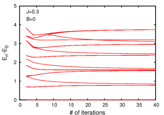
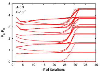
Figure 3: Finite size spectrum of the $S=1$ underscreened Kondo problem in the even sector in the absence (a) and presence (b) of a magnetic field. In the absence of a magnetic field the fixed point spectrum is that of a free Fermion field twisted by a phase shift $\pi/2$, and a residual spin $S^{*}=1/2$. In a magnetic field a second scale appears below which the fluctuations of the residual spin $S^{*}=1/2$ are frozen, and the spectrum can be characterized by a single, field-dependent phase shift $\delta(H)$.

Thus in the absence of a magnetic field fermions at the Fermi energy simply acquire a phase shift $\pi/2$. As a consequence, the spectrum of Eq. (18) is gapped for a finite system size, and the ground state of the system is only two-fold degenerate due to the presence of the residual spin $S^{*}$. As shown in Fig. 3.b, in the presence of a small magnetic field $H$ a new scale $\sim H$ emerges, below which the fluctuations of the residual spin are frozen out, and the ground state degeneracy is lifted. Below this scale the spectrum can be described simply by Eq. (18) with the modified boundary conditions

$$\tilde{\psi}_{\sigma}(-L/2)=-e^{-i2\delta_{\sigma}(H)}\tilde{\psi}_{\sigma}(L/2)\;,$$ (20)

where $\delta_{\sigma}(H)$ denote field-dependent phase shifts. Note that these phase shifts are the phase shifts of charged excitations, i.e., from the NRG spectrum we determine directly the phase shifts of the electrons at the Fermi energy.

We can thus determine the magnetic field dependence of the phase shifts directly from the NRG spectrum. As shown in shown in Fig. 4, the phase shifts approach $\pi/2$ as $0.29/{\rm ln}(T_{K}/H)$ in good agreement with the Bethe-Ansatz result for $S=1$ Eq.(16). In the inset of Fig. 4 we plotted the derivative of the phase shift too, that we computed by numerically differentiating the NRG results. This derivative is proportional to the quasiparticle density of states at the Fermi level, and indeed diverges approximately as $\sim 1/H$ for $H\to 0$.

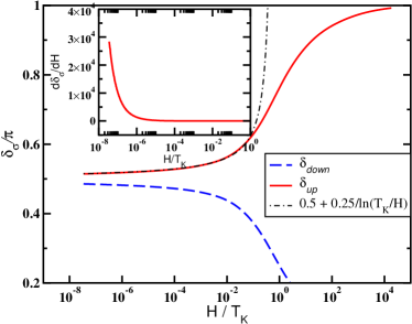
Figure 4: Magnetic field dependence of the phase shifts extracted from the NRG finite size spectrum. The phase shifts scale to $\pi/2$ as $\sim 1/{\rm ln}(T_{K}/|H|)$. Inset: The derivative of the phase shift diverges as $1/|H|$ for $|H|\ll T_{K}$.

V The Breakdown of Nozières’ Fermi Liquid Picture for the UKM

In his seminal papers noz , Nozières argued that one could perform a “Fermi Liquid expansion of phase shifts” at strong coupling. He argued that since the impurity is frozen into a singlet at strong coupling, the only remaining degrees of freedom in the problem were those of the Fermi liquid. He showed that all the physics could be captured by examining the phase shifts of quasi-particles as they pass the impurity. We shall now argue that this picture is valid for RFL but fails in the case of SFL.

Nozières’ prescription to describe a Fermi liquid is to assume that the phase shift for a quasiparticle of energy $\omega$ and spin $\sigma$ has the general form

$$\delta_{\sigma}(\omega)=\delta_{\sigma}[\omega,\{n_{\sigma^{\prime}}(\omega^{\prime})\}]\;,$$ (21)

where $\{n_{\sigma^{\prime}}(\omega^{\prime})\}$ denotes the occupation number of all other quasiparticle states. It is not clear from Nozières original paper how exactly the phase shift can be defined for a particle of finite energy, which scatters generically inelastically off the impurity. Implicitly, Nozières’ prescription assumes, that sufficiently close to the Fermi surface the inelastic scattering of a quasiparticle of energy $\omega$ is suppressed as $\sim\omega^{2}$, and thus quasiparticles are indeed well-defined. With this assumption, and assuming further that in the strong coupling fixed point everything is analytic near the Fermi surface one can proceed and expand the phase shift in powers of $\omega$ and the change of quasiparticle occupation number, $\delta n$, as

$$\delta_{\sigma}(\omega) = \delta_{0}(\omega)+\sum_{\omega^{\prime},\sigma^{\prime}}\phi_{\sigma,\sigma^{\prime}}(\omega,\omega^{\prime})\delta n_{\sigma^{\prime}}(\omega^{\prime})\;,$$

$$\delta_{0}(\omega) = \delta_{0}+\alpha\omega+\beta\omega^{2}\;,$$ (22)

where for the sake of simplicity we assumed $H=0$. These equations are the main constituents of Nozières’ Fermi liquid theory. The assumption that $\delta_{0}(\omega)$ is analytical in $\omega$ implies that the impurity-induced DOS remains finite at the Fermi energy with $\alpha\sim 1/T_{K}$.

Our Bethe Ansatz solution, however, shows that in the absence of a magnetic field the spinon phase shifts take the form

$$\delta_{s}(\omega)=\frac{\pi}{2}+\gamma\frac{\hbox{sign}(\omega)}{\ln\left(\frac{T_{K}}{\omega}\right)}+\dots\;,$$ (23)

leading to the singular density of states for the spinon excitations shown in Fig. 2,

$$N_{s}(\omega)=\frac{1}{\pi}\frac{\partial\delta_{s}}{\partial\omega}=\frac{\gamma}{\pi|\omega|\left(\log\left(\frac{T_{K}}{\omega}\right)\right)^{2}}\;.$$ (24)

As a results the conventional Fermi liquid expansion of the phase shift can not be carried out.

Another essential feature of the Nozières Fermi liquid approach, is the assumption of adiabaticity - that the excitations of the interacting system can be mapped onto the excitations of a corresponding non-interacting impurity problem. Since the interacting and non-interacting systems contain the same quasi-particles, the difference between the two situations can only be due to scattering by a one-particle potential.

We are thus lead to ask whether there is adiabaticity in the UKM. In light of the above observation, we can phrase the question in an alternative manner - is there any non-interacting scattering potential that can give rise to the observed energy-dependent spinon phase shift? In a conventional impurity scattering problem, the scattering potential and the phase shift are related by the relation

$$\delta(\omega)=\tan^{-1}[-\pi V(\omega)\rho]$$ (25)

where $V(\omega)$ is the bare scattering potential at energy $\omega$  Nozphase , so that

$$V(\omega)=-\frac{1}{\pi\rho}\tan\delta(\omega)$$ (26)

In the Nozières expansion, we have

$$\delta=\frac{\pi}{2}+\alpha\omega$$ (27)

so that the corresponding potential is given by

$$V(\omega)=\frac{1}{\pi\rho\alpha}\frac{1}{\omega}.$$ (28)

A $1/\omega$ phase shift indicates the formation of single bound-state inside the Kondo resonance. In fact, the scattering potential (28) is the same as that of a simple resonant level model with a resonance of width $\Gamma\sim\alpha^{-1}\sim T_{K}$ positioned right at the Fermi energy, $\epsilon_{d}=0$, implying that we can indeed map the excitations of the fluid onto a non-interacting Anderson impurity model.

If we now carry out the same procedure on the phase shift of the UKM, we find that

$$V^{*}(\omega)=\frac{1}{\pi\rho\gamma}\left[\ln\left(\frac{T_{K}}{\omega}\right)\right]\hbox{sign}(\omega)$$ (29)

This singular elastic scattering potential can not be replaced by a simple scattering pole, but would require an singular distribution of non-interacting scattering resonances for its correct description. In this way, we see that the singular Fermi liquid of the underscreened model can not be obtained from the adiabatic evolution of a simple, non-interacting impurity model.

VI Conclusion

We end our discussion by remarking on some interesting lines for future research. The UKM model discussed here is isotropic, and the characteristic scale for the field-tuned Fermi liquid is, up to a logarithm, a linear function of the magnetic field. It may be particularly interesting in future work to examine the properties of the anisotropic UKM

$$H_{UKM}=-i\int dx\,\psi^{\dagger}(x)\partial\psi(x)$$

$$+ J_{z}\left(\psi^{{\dagger}}(0){\sigma}_{z}\psi(0)\right){S}_{z}+J_{\perp}\left(\psi^{{\dagger}}(0){\sigma}_{\perp}\psi(0)\right){S}_{\perp}\;.$$

The low-temperature physics of this model maps onto an anisotropic ferromagnetic Kondo model at strong coupling, where the physics is described by a line of fixed points TG . In this problem, we expect that the linear specific heat coefficient will diverge with an exponent that depends on the degree of anisotropy,

$$\frac{C_{v}(T)}{T}\sim\frac{1}{T^{\alpha(J_{z}/J)}}\phi(\frac{T}{B})$$ (31)

where $\phi(x)$ is a scaling function. This kind of behavior has recently been seengegenwart ; Custers in the field-tuned QCP of YbRh₂Si₂, and the anisotropic underscreened Kondo model may provide an interesting point of comparison with the field tuned physics in anisotropic quantum critical systems.

Finally, in the spirit of the Nozières picture, Affleck and Ludwig have analyzed the low energy behavior of Kondo impurity models in the framework of boundary conformal field theory (BCFT)  Affleck . In this method, the various fixed points correspond to different conformally invariant boundary conditions. Although the over-screened and exactly-screened Kondo models were analyzed in great detail, the UKM were never properly examined, and it is still an open question how to incorporate the SFL behavior of the UKM we have found in terms of BCFT.

VII Acknowledgements

We have benefited from discussions and email exchanges with many people, including E. Boulat and I. Paul. This work has been supported by NSF through grants DMR 9983156 and DMR 0312495, by the Bolyai foundation, the NSF-MTA-OTKA Grant No. INT-0130446, and Hungarian grants No. OTKA T038162, T046303, and T046267 and the EU ‘Spintronics’ RTN HPRN-CT-2002-00302.

Appendix A Appendix 1: Calculation of DOS

In this appendix, we outline the calculation of the DOS for a spin-S, single channel Kondo model. As discussed in the text (11), the DOS is given by the derivative of the phase shift with respect to the energy excitation which can be rewritten as

$$\frac{d\delta_{s}}{d\omega}=\left(\frac{d\omega_{s}}{d\Lambda^{h}}\right)^{-1}\frac{d\delta_{s}}{d\Lambda^{h}}=\left(\frac{d\omega_{s}}{d\Lambda^{h}}\right)^{-1}\sigma_{im,B}(\Lambda^{h})$$ (32)

where $\omega$ is the excitation energy of the spinon and $\Lambda^{h}$ is the hole induced in the spin-rapidity due to the presence of a spinon. Hence, the calculation naturally divides into two parts, calculation of $\sigma_{im}(\Lambda)$ and the calculation of the excitation energy $\omega$.

We first concentrate on calculating $\sigma_{im}(\Lambda)$. Since, $\sigma_{im}(\Lambda)$ is not affected by the presence of the spinon, we can calculate $\sigma_{im}(\Lambda)$ directly in the ground state. The starting point for the calculation is the equation for the ground state in the presence of a magnetic field  footnote2

$$\sigma_{B}(\Lambda)+\int_{\Lambda_{B}}^{\infty}d\Lambda^{\prime}K(\Lambda-\Lambda^{\prime})\sigma_{B}(\Lambda^{\prime})=f(\Lambda)$$ (33)

As explained in the text, $\Lambda$ is the spin-rapidity and $\Lambda_{B}$ is a parameter related to the physical magnetic field, $H$, by the relation $\frac{H}{T_{k}}=\left(\frac{2}{\pi e}\right)^{1/2}e^{\pi/c\Lambda_{B}}$ where $T_{k}$ the Kondo temperature.

Shifting the limits of the integral and defining $\rho(\Lambda)=\sigma_{B}(\Lambda+\Lambda_{B})$ the above can be rewritten as

$$\rho(\Lambda)+\int_{0}^{\infty}d\Lambda^{\prime}K(\Lambda-\Lambda^{\prime})\rho(\Lambda^{\prime})=f(\Lambda+\Lambda_{B})$$ (34)

This equation can be solved using the Weiner-Hopf technique. This technique relies on separating all expressions into a sum of expressions that have singularities only in either the upper of lower half-plane. After separating all the expressions, one can equate those expressions that are analytic in each half-plane separately.Most of the manipulations in the appendix are performed in order to facilitate this separation. To proceed, define $\rho_{\pm}(\Lambda)=\theta(\pm\Lambda)\rho(\Lambda)$. Then, (34) becomes

$$\rho_{+}(\Lambda)+\rho_{-}(\Lambda)+\int_{-\infty}^{\infty}d\Lambda^{\prime}K(\Lambda-\Lambda^{\prime})\rho_{+}(\Lambda^{\prime})=f(\Lambda+\Lambda_{B})$$ (35)

Taking the Fourier Transform of the above and noting that the integral is a convolution one has the equation

$$\tilde{\rho}_{+}(p)\left(1+\tilde{K}(p)\right)+\tilde{\rho}_{-}(p)=\tilde{f}(p)e^{ip\Lambda_{B}}$$ (36)

One now wants to separated the terms in the above equation into functions with singularities only in the upper/lower half plane. Hence, one rewrites the above equation as

$$1+\tilde{K}(p)=\frac{K_{+}(\frac{cp}{2\pi})}{K_{-}(\frac{cp}{2\pi})}$$ (37)

where $K_{+}(K_{-})$ have singularities only in the upper(lower) half plane. Explicitly, one has

$$K_{+}(q)=K_{-}^{-1}(-q)$$

$$=\frac{(2\pi)^{1/2}}{\Gamma(\frac{1}{2}+iq)}\exp\left[-iq\left[1+\frac{i\pi}{2}-\log{(-q+i\epsilon)}\right]\right]$$ (38)

Equation (36) can be rewritten as

$$\tilde{\rho}_{+}(p)K_{+}(\frac{cp}{2\pi}) +\tilde{\rho}_{-}(p)K_{-}(\frac{cp}{2\pi})$$ (39)

$$=K_{-}(\frac{cp}{2\pi})\tilde{f}(p)e^{ip\Lambda_{B}} \Lambda_{B}\geq 0$$

$$=K_{+}(\frac{cp}{2\pi})\tilde{g}(p)e^{ip\Lambda_{B}} \Lambda_{B}\leq 0$$

where

$$\tilde{f}(p) = N^{e}e^{-c/2|p|}+N^{i}e^{-cs|p|}$$

$$\tilde{g}(p) = \frac{\tilde{f}(p)}{1+\tilde{K}(p)}=\frac{N^{e}e^{ip}+N^{i}e^{(S-1/2)|p|}}{2{\cosh\left(\frac{c}{2}p\right)}}$$ (40)

Inverse Fourier transforming the above expression for $\tilde{g}(p)$, one has

$$g(\Lambda)=\frac{1}{2c}\frac{N^{e}}{{\cosh\left(\frac{\pi}{c}(\Lambda-1)\right)}}+\sum_{k=0}^{\infty}N^{i}\frac{(-1)^{k}c(S+k)}{c(S+k)^{2}+\Lambda^{2}}.$$ (41)

Since we are interested in small magnetic fields, we concentrate on the $\Lambda_{B}\leq 0$ solutions. In order to separate the right hand side of ( 39) into parts that have singularities only in one half-plane, it is useful to rewrite $\tilde{g}(p)$ in an alternative way. To do this, we follow  natan and Laplace transform the above expression for $g(\Lambda)$ to get

$$g(\Lambda)=\sum_{k=0}^{\infty}(-1)^{k}\left(\frac{N^{e}}{c}e^{-\frac{\pi}{c}(2k+1)|\Lambda-1|}+N^{i}\int_{0}^{\infty}dt{\sin\left(c(S+k)t\right)}e^{-|\Lambda|t}\right)$$ (42)

Since we are interested in $\tilde{g}(p)$, we Fourier transform each amplitude of the Laplace transform separately. Define $\tilde{g}_{t}(\Lambda)=e^{-|\Lambda|t}$. Its Fourier transform is given by

$$\tilde{g}_{t}(p)=i\left(\frac{1}{p+it}-\frac{1}{p-it}\right)$$ (43)

Notice that each term in ( 39) can be written as an sum or integral of terms of the form $K_{+}\left(\frac{cp}{2\pi}\right)\tilde{g}_{t}(p)e^{ip\Lambda_{B}}$. We want to write each term as a sum of functions that have singularities solely in the upper/lower half-plane. Define $\tilde{\rho}_{\pm}(p,t,\Lambda_{B})$ to be

$$\tilde{\rho}_{\pm}(p,t,\Lambda_{B})=\frac{q_{\pm}^{{}^{\prime\prime}}(p,t,\Lambda_{B})}{K_{\pm}(p)}$$ (44)

where

$$q_{+}^{{}^{\prime\prime}}(p,t,b)= (-i)K_{+}\left(\frac{cp}{2\pi}\right)\frac{e^{ip\Lambda_{B}}}{p-it}+i\left[K_{+}\left(\frac{cp}{2\pi}\right)e^{ip\Lambda_{B}}-K_{+}\left(\frac{-ict}{2\pi}\right)e^{\Lambda_{B}t}\right]\frac{1}{p+it}$$ (45)

$$q_{-}^{{}^{\prime\prime}}(p,t,b)= iK_{+}\left(\frac{-ict}{2\pi}\right)\frac{e^{\Lambda_{B}t}}{p+it}$$ (46)

Note that $\tilde{\rho}_{+}(p,t,\Lambda_{B})$ [$\tilde{\rho}_{-}(p,t,\Lambda_{B})$] has singularities only in the upper (lower) half p-plane. Then,

$$\rho_{\pm}(p)=\sum_{k=0}^{\infty}(-1)^{k}\left[\frac{N^{e}}{c}\tilde{\rho}_{\pm}\left(p,t=(2k+1)\frac{\pi}{c},\Lambda_{B}-1\right)+\frac{N^{i}}{\pi}\int_{o}^{\infty}dt\,{\sin\left(c(S+k)t\right)}\tilde{\rho}_{\pm}\left(p,t,\Lambda_{B}\right)\right]$$ (47)

Since we want to calculate $\sigma_{im}$, the density of states at the impurity, we can simply concentrate only on the part of the above expression that is proportional to $N_{i}$. Inverse transforming the above expressions and adding them one has

$$\rho_{im}(\Lambda) = N^{i}\sum_{k=0}^{\infty}(-1)^{k}\int_{0}^{\infty}dt\,{\sin\left(c(s+k)t\right)}\frac{1}{2\pi i}\left[\int_{-\infty}^{\infty}dp\,\frac{e^{ip(\Lambda+\Lambda_{B})}}{p-it}-\frac{e^{ip(\Lambda+\Lambda_{B})}}{p+it}\right]$$ (48)

$$+ N^{i}\int_{0}^{\infty}dt\,{\sin\left(ct(S+k)\right)}\frac{1}{2\pi i}\left[\int_{-\infty}^{\infty}dp\,e^{-ip\Lambda}e^{\Lambda_{B}t}K_{+}(ict/2\pi)\frac{K_{+}(cp/2\pi)-K_{-}(cp/2\pi)}{p-it}\right]$$

From now on we will be concerned exclusively with the impurity portion Noting that $\sigma_{B,im}(\Lambda+\Lambda_{B})=\rho_{im}(\Lambda)$ one can write

$$\sigma_{im,B}(\Lambda)=\sigma_{im,H=0}(\Lambda)+\sigma_{im,H\neq 0}(\Lambda)$$

where we have separated the impurity density into a zero-field, $\sigma_{im,H=0}(\Lambda)$ and finite-field contribution, $\sigma_{im,H\neq 0}(\Lambda)$. Explicitly, these are given by

$$\sigma_{im,H=0}(\Lambda) = N^{i}\sum_{k=0}^{\infty}(-1)^{k}\int_{0}^{\infty}dt\,{\sin\left(c(S+k)t\right)}\frac{1}{2\pi i}\left[\int_{-\infty}^{\infty}dp\,\frac{e^{ip\Lambda}}{p-it}-\frac{e^{ip\Lambda}}{p+it}\right]$$ (49)

$$= \sum_{k=0}^{\infty}\frac{(-1)^{k}c(S+k)}{\left[c(S+k)\right]^{2}+\Lambda^{2}}$$

and

$$\sigma_{im,H\neq 0}(\Lambda)=N^{i}\sum_{k=0}^{\infty}(-1)^{k}\int_{0}^{\infty}dt\,{\sin\left(ct(S+k)\right)}\frac{1}{2\pi i}\left[\int_{-\infty}^{\infty}dp\,e^{-ip(\Lambda-\Lambda_{B})}e^{\Lambda_{B}t}K_{+}(ict/2\pi)\frac{K_{+}(cp/2\pi)-K_{-}(cp/2\pi)}{p-it}\right]$$ (50)

For what follows, we assume $\Lambda_{B}\ll 0$ or the physical magnetic field $H/T_{k}\ll 1$. In equation (50), the integral over t is dominated by t very close to zero. Hence, we can substitute t=0 in $K_{+}$ integrate over t to get the expression

$$\sigma_{im,H\neq 0}(\Lambda)=N^{i}\sum_{k=0}^{\infty}\frac{(-1)^{k}c(S+k)}{c^{2}(S+k)^{2}+\Lambda_{B}^{2}}\times\frac{1}{2\pi i}\left[\int_{-\infty}^{\infty}dp\,e^{-ip\frac{\pi}{c}(\Lambda-\Lambda_{B})}\frac{K_{+}(p/2)-K_{-}(p/2)}{p-i\epsilon}\right]$$ (51)

We close the contour below and noting that the poles in $K_{-}$ arise from Gamma function one has in the universality limit:

$$\sigma_{H\neq 0}(\Lambda)=N^{i}\sum_{k=0}^{\infty}\frac{(-1)^{k}c(S+k)}{c^{2}(S+k)^{2}+\Lambda_{B}^{2}}\times\frac{e^{-\frac{\pi}{c}(\Lambda-\Lambda_{B})}}{\sqrt{2\pi e}}$$ (52)

Hence, for $H<<T_{k}$, the expression for the impurity density $\sigma_{im,B}(\Lambda)$ in the presence of a magnetic field is given by

$$\sigma_{im,B}(\Lambda)=N^{i}\sum_{k=0}^{\infty}\left[\frac{(-1)^{k}c(S+k)}{c^{2}(S+k)^{2}+\Lambda^{2}}+\frac{(-1)^{k}c(S+k)}{c^{2}(S+k)^{2}+\Lambda_{B}^{2}}\times\frac{e^{-\frac{\pi}{c}(\Lambda-\Lambda_{B})}}{\sqrt{2\pi e}}\right]$$ (53)

Having calculated, $\sigma_{im,B}(\Lambda)$, in order to calculate the DOS, we must now calculate $\left(\frac{d\omega}{d\Lambda^{h}}\right)$ where $\omega$ is the excitation energy of the spinon excitation and depends explicitly on the hole position $\Lambda^{h}$. To calculate spinon energy one starts with the BAE equation in the presence of a hole

$$\sigma_{B}(\Lambda)+\delta(\Lambda-\Lambda^{h})+\int_{\Lambda_{B}}^{\infty}K(\Lambda-\Lambda^{\prime})\sigma_{B}(\Lambda^{\prime})d\Lambda^{\prime}=f(\Lambda)$$ (54)

Define $\Delta\sigma_{B,\Lambda^{h}}(\Lambda)$, the change in the spin-rapidity due to the hole, by

$$\sigma_{B}(\Lambda)+\delta(\Lambda-\Lambda^{h})=\sigma_{B,gs}(\Lambda)+\Delta\sigma_{B,\Lambda^{h}}(\Lambda).$$ (55)

Substituting the above definition into (54) and using (33) one has,

$$\Delta\sigma_{B}(\Lambda)+\int_{\Lambda_{B}}^{\infty}\Delta\sigma_{B}(\Lambda^{\prime})K(\Lambda-\Lambda^{\prime})d\Lambda^{\prime}=K(\Lambda-\Lambda^{\prime})$$

Shifting the integral, taking the Fourier Transform, and rewriting in terms of $K_{\pm}(p)$ one has

$$e^{ip\Lambda_{B}}\tilde{h}(p)=K_{+}(\frac{cp}{2\pi})\Delta\tilde{\rho}_{+}(p)+K_{-}(\frac{cp}{2\pi})\Delta\tilde{\rho}_{-}(p)=\frac{e^{-c|p|}e^{-ip(\Lambda^{h}-\Lambda_{B})}}{1+e^{-c|p|}}=e^{-ip(\Lambda^{h}-\Lambda_{B})}\sum_{k=o}^{\infty}(-1)^{k}e^{-c(k+1)|p|}$$ (56)

where we have defined a new function $h(\Lambda)$ whose Fourier transform is given by the expression $\tilde{h}(p)$ above. Explicitly,

$$h(\Lambda)=\frac{1}{4}\sum_{k=1}^{\infty}(-1)^{k+1}\frac{ck}{(ck)^{2}+(\Lambda-(\Lambda^{h})^{2})}$$ (57)

In analogy with the manipulations we used for the second term in (40) when calculating the DOS, we write $h(\Lambda)$ as a Laplace transform, Fourier transform each Laplace component, and then equate functions with singularities only in the upper and lower half planes to get

$$\Delta\tilde{\sigma}_{-}(p)=\sum_{k=0}^{\infty}(-1)^{k}\int_{0}^{\infty}dt\;{\sin(c(k+1)t)}i\frac{K_{+}\left(\frac{-ict}{2\pi}\right)e^{-ip\Lambda_{B}}}{K_{-}\left(\frac{cp}{2\pi}\right)}\frac{e^{-(\Lambda^{h}-\Lambda_{B})t}e^{\Lambda_{B}t}}{p+it}$$ (58)

and

$$\Delta\tilde{\sigma}_{+}(p)=\frac{1}{4}\sum_{k=1}^{\infty}(-1)^{k+1}\int_{0}^{\infty}dt\;{\sin(ckt)}(-i)\left[\frac{e^{-ip\Lambda^{h}}}{p-it}-\frac{e^{-ip\Lambda^{h}}}{p+it}+\frac{e^{-(\Lambda^{h}-\Lambda_{B})t}e^{-ip\Lambda_{B}}}{p+it}\frac{K_{+}(-ict/2\pi)}{K_{+}(cp/2\pi)}\right]$$ (59)

The excitation energy is given by ($D=N^{e}/L$ is the bandwidth)

$$\omega(\Lambda^{h})=D\int_{\Lambda_{B}}^{\infty}d\Lambda\,\Delta\sigma_{+}(\Lambda)\left[\theta(2\Lambda-2)-\pi\right]-H\int_{-\infty}^{\Lambda_{B}}d\Lambda\Delta\sigma_{-}(\Lambda)$$ (60)

To proceed, note that the second term can be rewritten as

$$H\int_{-\infty}^{\Lambda_{B}}d\Lambda\Delta\sigma_{-}(\Lambda)=\int_{-\infty}^{0}d\Lambda\Delta\rho_{-}(\Lambda)=\int_{-\infty}^{\infty}d\Lambda\Delta\rho_{-}(\Lambda)=H\Delta\tilde{\rho}_{-}(0)$$ (61)

For, very small $H\Delta\tilde{\rho}_{-}(0)$ tends to $H^{\prime}=H(\frac{e}{2\pi})^{1/2}$. After some manipulations, the first term can be written

$$\omega(\Lambda^{h}) = \int_{0}^{\infty}dp-\frac{{\sin(p\Lambda^{h})}}{(1+e^{cp})p}e^{-cp/2}+\frac{\pi}{2}$$ (62)

$$+ \frac{1}{4}\sum_{k=1}^{\infty}(-1)^{k+1}\int_{0}^{\infty}dt{\sin(ckt)}\frac{e^{-(\Lambda^{h}-\Lambda_{B})t}e^{-ip\Lambda_{B}}e^{-c|p|/2}}{p(p+it)}\frac{K_{+}(-ict/2\pi)}{K_{+}(cp/2\pi)}-H^{\prime}$$

The sum of the first two terms in the expression above is the the expression for the excitation energy for zero field. Hence, we know that in the universality limit

$$\omega(\Lambda^{h})=2T_{0}e^{\pi/c\Lambda^{h}}+\sum_{k=1}^{\infty}(-1)^{k}\int_{0}^{\infty}dt{\sin(ckt)}K_{+}(-ict/2\pi)e^{-\Lambda^{h}t}e^{\Lambda_{B}t}\left[\frac{H}{\sqrt{2}t}+\int_{-\infty}^{\infty}dp\frac{e^{-ip\Lambda_{B}}e^{-c|p|/2}}{p(p+it)K_{+}(cp/2\pi)}\right]-H^{\prime}$$ (63)

For $B\ll 0$ (very small fields), we can ignore the second term giving us the result:

$$\frac{d\omega}{d\Lambda^{h}}=T_{0}\frac{\pi}{c}e^{\pi/c\Lambda^{h}}$$ (64)

Hence we see that the DOS of spinons at the impurity is given by:

$$N_{s}(\omega(\Lambda^{h}))=\frac{c}{\pi^{2}T_{K}}\sum_{k=0}^{\infty}\left[e^{-\pi/c\Lambda^{h}}\frac{(-1)^{k}c(S+k)}{c^{2}(S+k)^{2}+{\Lambda^{h}}^{2}}+\times\frac{e^{-\pi/c(2\Lambda^{h}-\Lambda_{B})}}{\sqrt{2\pi e}}\frac{(-1)^{k}c(S+k)}{c^{2}(S+k)^{2}+\Lambda_{B}^{2}}\right]+\mathcal{O}(H)$$ (65)

where it is implicitly assumed that $\Lambda^{h}>\Lambda_{B}$ We can rewrite the above equation

$$N_{s}(\omega(\Lambda^{h}))=\frac{1}{2\pi^{2}T_{k}}\left(e^{-\frac{\pi}{c}\Lambda^{h}}{\rm Re\,}[\beta(S+i\Lambda^{h}/c)]+\frac{e^{-\pi/c(2\Lambda^{h}-\Lambda_{B})}}{\sqrt{2\pi e}}{\rm Re\,}[\beta(S+i\Lambda_{B}/c)]\right)$$ (66)

where Re [f] denotes the real part of f and

$$\beta(x)=\frac{1}{2}\left(\psi(\frac{x+1}{2})-\psi(\frac{x}{2})\right)$$ (67)

Here, $\psi(x)$ is the DiGamma function. From (63), one has the following relation between the physical excitation energy $\omega$ and $\Lambda^{h}$, $(\omega+H^{\prime})/T_{k}=e^{\frac{\pi}{c}\Lambda^{h}}$ where as before $H^{\prime}=(\frac{e}{2\pi})^{1/2}H$ . Note that as always, $\omega$ is measured from the Fermi-surface Combining this with the previously stated relation between $B$ and $H$ the DOS becomes

$$N(\omega)=\frac{1}{2\pi^{2}}\left(\frac{1}{\omega+H^{\prime}}{\rm Re\,}[\beta(S+i\frac{1}{\pi}\log{((\omega+H^{\prime})/T_{k})})]+\frac{H}{2\pi(\omega+H^{\prime})^{2}}{\rm Re\,}[\beta(S+i\frac{1}{\pi}\log{(H^{\prime}/T_{k})})]\right)$$ (68)

References

- (1) P. Nozières, Journal de Physique C 37, C1-271, (1976); P. Nozières, J. Low Temp. Phys. 17, 31 (1974).
- (2) I. Affleck and A.W.W. Ludwig, Physical Review B, 48, 7297 (1993).
- (3) A.C.Hewson, The Kondo Problem to Heavy Fermion, (Cambridge Univ.,1993).
- (4) P. D. Sacramento and P. Schlottmann, J. Phys. Cond. Matter 3, 9687 (1991);P. D. Sacramento and P. Schlottmann, Phys. Rev. B 40, 431 (1989)
- (5) P. Coleman and C. Pepin, Physical Review B, 68 220405 (2003).
- (6) P. W. Anderson, Phys. Rev. 124, 41, 1961. J. Kondo, Prog. Theoret. Phys., 32, 37, 1964; ibid., 28, 772, 1962. B. Coqblin and J. R. Schrieffer, Phys. Rev. 185, 847, 1969. Anderson P. W. & G. Yuval, Phys. Rev. Lett. 45, 370, 1969; Phys. Rev. B 1, 1522, 1970; Journal of Phys. 4, 607, 1971. K. G. Wilson, Rev. Mod phys. 47, 773, 1976. P. Nozières, Journal de Physique, 37, C1-271, 1976 ; P. Nozières and A. Blandin, Journal de Physique 41, 193, 1980.
- (7) S. Doniach, Physica B 91, 231 (1977).
- (8) N. Read & D. M. Newns, Journal of Physics C 29, L1055, 1983 ; ibid 18, 2051, 1985. P. Coleman, Phys. Rev. B 28, 5255, 1983, ibid 29, 3035, 1984. A. Auerbach and K.Levin,Phys. Rev. Lett. 57, 877, 1986. A.J. Millis and P.A. Lee, Phys. Rev. B 35, 3394, 1986.
- (9) A. Schiller, F. B. Anders, and D. L. Cox ,Phys. Rev. Lett. 81, 3235 (1998). M. Koto, D.L. Cox, Phys. Rev. Lett. 82, 2575 (1999).
- (10) P. Coleman, C. Pepin, R. Ramazashvili and Q. Si, J. Cond Matt,13, R723 (2001).
- (11) P.Gegenwart, J. Custers, C. Geibel, K. Neumaier, T. Tayama, K. Tenya, O. Trovarelli, F. Steglich, Phys. Rev. Lett. 89 056402 (2002).
- (12) J. Custers, P. Gegenwart, H. Wilhelm, K. Neumaier, Y. Tokiwa, O. Trovarelli, C. Geibel, F. Steglich, C. Pepin, P. Coleman Nature, 424, 524 (2003).
- (13) C. Itzikson and J.B. Zuber, Quantum Field Theory (McGraw-Hill, 1985).
- (14) J. M. Maldacena and A. W. W. Ludwig, Nucl. Phys. B506, 565 (1997).
- (15) J. von Delft, G. Zaránd, and M. Fabrizio, Phys. Rev. Lett. 81, 196 (1998).
- (16) G. Zarand, L. Borda, Jan von Delft, and N. Andrei cond-mat/0403696
- (17) A. Zawadowski, J. von Delft, and D. C. Ralph, Phys. Rev. Lett. 83, 2632 (1999).
- (18) Note that the assumption of Ref. JanZar, , that the single particle scattering cross section vanishes in the limit is incorrect. The intereference of the unscattered electron waves with the elastically scattered portion of their wave function yields a complete cancellation for out-going single particle states.
- (19) V. A. Fateev and P. B. Wiegmann,Phys. Rev. Lett. 46 1595 (1981).
- (20) K. Furuya and J. H. Lowenstein, Phys. Rev. B 25, 5935 (1982).
- (21) N. Andrei, K. Furuya and J. H. Lowenstein, Rev. Mod. Phys. , Vol.55 331 (1983).
- (22) N. Andrei, Phys. Lett. A 87, 299 (1981).
- (23) D.C. Langreth Phys Rev. 150, 516 (1966).
- (24) N. Andrei and J. H. Lowenstein, Phys. Lett. B 91 401, 1980.
- (25) N. Andrei, Integrable Models in Condensed Matter Physics, in Series on Modern Codensed Matter Physics - Vol. 6, 458 - 551, World Scientific, Lecture Notes of ICTP Summer Course 1992. Editors: S. Lundquist, G. Morandi and Yu Lu. cond-mat/9408101.
- (26) For details, please consult the review (Andrei, Furuya, and Lowenstein).
- (27) Alternatively, one can think about adding an electron to the system and seeing the effect this has on the density of solutions. From simple counting arguments, it can be shown that adding an electron corresponds to creating a hole in the density. Hence, at low energies, the electron can be identified with a spinon.
- (28) N. Andrei and J.H. Lowenstein Phys. Rev. Lett 46 356 (1981)
- (29) K. Wilson Rev. Mod. Phys. 47, 773 (1975).
- (30) P. Nozières Journal de Physique 39, 1118 (1978).
- (31) T. Giamarchi, C. M. Varma, A. E. Ruckenstein and P. Nozières, Phys. Rev. Lett. 70, 3967 (1993).
- (32) I. Affleck and A. Ludwig, Nucl. Phys. B360 641 (1991); I. Affleck and A. Ludwig, Phys. Rev. Lett. 67, 161 (1991). (1997).