Dynamics of simple liquids at heterogeneous surfaces : Molecular Dynamics simulations and hydrodynamic description

Abstract

In this paper we consider the effect of surface heterogeneity on the slippage of fluid, using two complementary approaches. First, MD simulations of a corrugated hydrophobic surface have been performed. A dewetting transition, leading to a super-hydrophobic state, is observed for pressure below a “capillary” pressure. Conversely a very large slippage of the fluid on this composite interface is found in this superhydrophobic state. Second, we propose a macroscopic estimate of the effective slip length on the basis of continuum hydrodynamics, in order to rationalize the previous MD results. This calculation allows to estimate the effect of a heterogeneous slip length pattern on the composite interface. Comparison between the two approaches are in good agreement at low pressure, but highlights the role of the exact shape of the liquid-vapor interface at higher pressure. These results confirm that small variations in the roughness of a surface can lead to huge differences in the slip effect. On the basis of these results, we propose some guidelines to design highly slippery surfaces, motivated by potential applications in microfluidics.

I Introduction

The question of the hydrodynamic boundary condition (h.b.c.) for simple fluids has received much attention recently, and a number of experimental studies have addressed this problem  Churaev84 ; watanabe99 ; Vinogradova99 ; Pit2000 ; Baudry2001 ; Craig2001 ; Granick2001 ; cheng2002 ; Granick2002 ; tretheway2002 ; Bonaccurso2002 ; lpmcn2002 ; Bonaccurso2003 ; VinoYabukov ; Breuer03 . Usually, when a simple liquid flows over a motionless solid wall, its velocity is assumed to be equal to zero near the wall. This assumption is a postulate of hydrodynamics. Although it is widely verified for macroscopic flows of simple fluids, its validity at small scales remains an open question. Wall slippage is usually described in terms of an extrapolation length, usually denoted as the slip length, b : this corresponds to the distance between the wall and the position at which the linear extrapolation of the velocity profile vanishes. Analytical calculations and numerical simulations have shown that two parameters mainly affect the h.b.c.: the roughness of the surface Richardson73 and the solid-liquid interaction Barrat99a ; Barrat99b ; Thompson97 . While roughness is usually expected to decrease slippage, hydrophobocity of the solid surface has been found to enhance the slip length. ¿From an experimental point of view, many studies have been carried out recently but they do not allow to draw a simple and unique conclusion concerning the effect of roughness and solid-liquid interaction on slippage, as a huge dispersion in the results is observed for seemingly similar systems. For instance, on “smooth” hydrophobic surfaces, slip lengths $b$ were obtained that range from a few nanometers Churaev84 up to a few micrometers tretheway2002 . Even at a qualitative level, some results appear to contradict each other. To cite an intriguing point as an exemple, roughness has be found either to increase Granick2002 or to decrease the slip length Bonaccurso2002 . It is therefore important to clarify this question from a fundamental point of view, in order to understand the origin of this important variability of results. ¿From a more “practical” perspective, the possibility for a liquid to slip over a solid surface can also have important consequences for flows in microchannels. A large slip length reduces dissipation at the surfaces and therefore affects the pressure drop in a given channel geometry. It also may help in reducing the hydrodynamic dispersion due to the velocity gradient between the center and the channel boundary, with important applications for exemple in chemical or biological techniques of analysis (micro-chromatography). Finally, slippage is also an important phenomenon for flows in mesoporous media, where the understanding of the effect of mechanical dissipation is essential for applications such as dampers lefevre .

In previous work naturemat , we have shown by Molecular Dynamics (MD) simulations that the slip length is strongly affected by the roughness of the substrate for non wetting solid-fluid interactions, a point which could explain some of the experimental discrepancies. In particular, we have found, for a non wetting patterned surface, a thermodynamic transition between two different surface states as a function of the pressure : a “normal” state where the liquid occupies all the available volume, and a “super-hydrophobic” state, where the liquid flows over the roughness. In the “normal” state, the h.b.c. is well described by a no slip condition (the roughness decreases the slip length), whereas the “super-hydrophobic” state enhances a slip h.b.c., with slip lengths greater than in the smooth case (the roughness increases the slip length).

Our aim in this paper is twofold. First, using MD simulations, we present a more detailed study of the transition between the “normal” and the “super-hydrophobic” state, as a function of the roughness parameters, geometry and pressure. Note that the geometry studied here consists of grooves with different widths and heights. This provides an ideal geometry, from which one could expect to extract simple rules. Slippage over the surface is conversely studied in the different thermodynamic states. Second, we try to rationalize the effect of the surface heterogeneity on the measured slip length, as observed in the previous MD simulations. To this end, we develop a macroscopic description of the hydrodynamic flow on a microscopically heterogeneous surface, characterized by a spatially varying h.b.c. Beyond the comparison to the MD results, this analysis allows us to propose an optimized surface heterogeneity, designed to obtain large slippage at the interface.

II Molecular Dynamics approach

II.1 Phase properties of heterogeneous surfaces

We consider in this study a liquid confined between two parallel solid walls. The bottom wall is decorated with a periodic array of grooves of height $h$ and width $a$. Note that this differs from the system considered in reference naturemat , where a periodic array of square dots had been considered. Periodic boundary conditions are used in the directions parallel to the walls, the length of a cell of simulation is $L$. In our simulations, all the interactions are of the Lennard-Jones type :

$$v_{ij}=4\epsilon\left[\left(\frac{\sigma}{r}\right)^{12}-c_{ij}\left(\frac{\sigma}{r}\right)^{6}\right]$$ (1)

The fluid and the solid atoms have the same molecular diameter $\sigma$ and interaction energies $\epsilon$. The variation in the $c_{ij}$ (the index $i,j=F,S$ refers to the fluid or solid phase) is a convenient control parameter that can be varied to adjust the surface tensions. The solid substrate is described by atoms fixed on a the (100) plane of an FCC lattice. We have worked with two values of $c_{FS}$, $c_{FS}=0.5$ or $c_{FS}=0.8$, which correspond to contact angles (deduced from Young’s law) of $\theta=137^{o}$ or $\theta=110^{o}$, respectively Barrat99b . The simulations are carried out at constant temperature $k_{B}T/\epsilon$=1. In flow experiments, the velocity component in the direction orthogonal to the flow was thermostatted Barrat99b , in order to avoid viscous heating within the fluid slab.

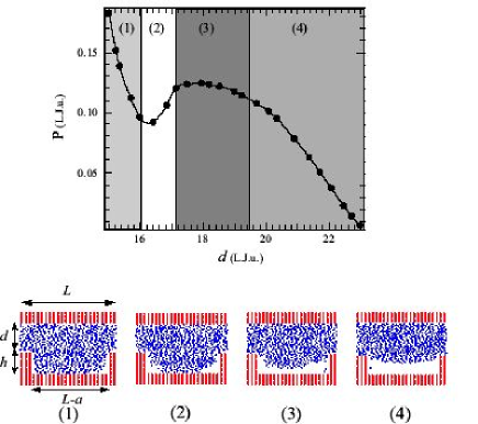
Figure 1: (a) Normal pressure P (in Lennard-Jones units) versus thickness of the cell $d$ (in Lennard-Jones units). The periodicity is $L=18.9\ \sigma$, the height of the grooves is $h=10.7\ \sigma$ and the width of the groove is $L-a=15.6\ \sigma$. (b) Transverse views of the atomic configuration for different situations. Atoms belonging to the liquid and solid are represented by points and round dots, respectively.

Figure 1 displays the evolution of the pressure with the distance $d$ between the walls of the cell. The normal pressure is obtained from the average force on the substrates along the $z$ direction. Since the number of atoms is kept constant, this plot is similar to a $P-V$ isotherm (pressure versus volume) in the bulk. We have verified that changing the pressure by modifying the number of particules in the cell at fixed volume $V$ leads to equivalent results. As for the case of dots naturemat , this isotherm exhibits two branches, separated by a “Van der Waals loop”, indicating a phase transition between two possible situations. As shown in figure 1, where transverse views of the atomic configurations for different pressures are represented, this transition corresponds to a partial dewetting of the space between the grooves. At high pressures, the liquid occupies all the cell (see figure 1), including the grooves. This state will be described in the following as the “normal” state. At lower pressures, partial dewetting is observed and a composite interface is formed. In the latter case, the space between the grooves is essentially free from liquid atoms (see figure 1). This state will be therefore denoted as the “super-hydrophobic” state. Note that the range of distances for which the pressure decreases with $d$ is thermodynamically unstable, its observation being merely an artefact of small size simulations.

Qualitatively, the maximum of the pressure on the previous Van der Waals loop corresponds to the capillary pressure $P_{cap}$, for which the liquid starts invading the grooves. On the other hand, the minimum corresponds to the pressure at which the liquid reaches the bottom of the groove and adapts its contact angle in order to satisfy Laplace’s law.

A qualitative interpretation of this dewetting transition can be given in terms of macroscopic capillarity. If we consider a system at fixed normal pressure $P_{N}$, the difference in Gibbs free energies between the normal state (case $A$) and the formation of a superhydrophobic state (case $B$) can be written as:

$$G_{B}-G_{A}=L\{(L-a+2h)\ (\gamma_{LV}cos\theta)+(L-a)\ \gamma_{LV}+P_{N}(L-a)h\}$$ (2)

The composite interface is therefore favored when

$$P_{N}<P_{composite}=P_{cap}+\frac{-\gamma_{LV}.(cos\theta+1)}{h}$$ (3)

where we have introduced the capillary pressure $P_{cap}$, defined as

$$P_{cap}=-\frac{2\gamma_{LV}cos\theta}{L-a}$$ (4)

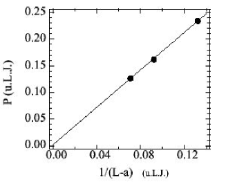
Figure 2: Measured capillary pressure $P_{cap}$ in the simulation (in Lennard-Jones units) as a function of the inverse groove width $1/(L-a)$. These results corresponds to grooves with sufficiently large depth, $h$, so that the measured capillary pressure becomes independent of $h$.

Although a quantitative agreement can hardly be expected in view of the small sizes in our system, we have checked that equation 3 correctly predicts the general trends observed in our simulation, when the height or width or the grooves are varied. As an example, we have plotted the measured capillary pressure on Fig. 2, here defined in the simulations as the maximum pressure for which the dewetted state is stable (corresponding to the local maximum in figure 1). This plot corresponds to the limit in which the grooves have a large depth $h$, so that the “composite” pressure, defined in equation (3) should reduce to the capillary pressure, equation (4). As shown in this figure, the linear dependence of the pressure as a function of $1/(L-a)$ does confirm the validity of the macroscopic argument above. Moreover, the slope of the linear fit agrees within $15\%$ with the predicted one, $2\gamma_{LV}cos\theta$ Barrat99b .

II.2 Slippage over heterogeneous surfaces

We now turn to the main point of the present paper, namely the slippage of the fluid on the previous heterogeneous surface.

We have conducted parallel Couette flow simulations. A shear flow is induced by moving the upper wall with velocity $U$ and the lower wall with a velocity $-U$. Typically we chose $U=0.3$ in reduced Lennard-Jones units. We have verified that, in spite of the large value of the velocity, the response is linear and the measured slip lengths are independent of the velocity $U$. Temperature is kept constant by thermostatting through velocity rescaling in the direction perpendicular to the flow. For flat walls Barrat99a , the slip length $b$ is defined as the distance between the wall position and the depth at which the extrapolated velocity profile reaches the nominal wall velocity, $v=U$. In the presence of grooves, the same definition is used. Obviously the presence of grooves makes the choice of the wall position somewhat arbitrary. We choose to define the wall as the position of the bottom layer of the substrate. This choice will be seen to have only a negligible influence on the results (since, as discussed below, the measured slip lengths are found to be much larger than the groove depth in the interesting “superhydrophobic” state).

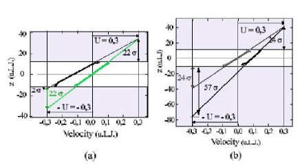
Figure 3: Velocity profile in a Couette flow (black lines) : (a) in the normal state (high pressure) where the liquid fills the grooves; (b) in the superhydrophobic state (low pressure) where the grooves are dewetted. The upper and lower wall have velocity $U=\pm 0.3$ (in Lennard-Jones units). The grey lines are the velocity profiles obtained for a smooth surface (i.e. no grooves) at the same pressure.

Typical measured velocity profiles are plotted in figure 3. As shown on this figure, the slippage strongly depends on the surface state : globally, while in the “normal” state the slip length is found to be very small (roughness reduces slip), in the “superhydrophobic” state the slip length is strongly enhanced compared to the smooth surfaces case (with the same solid-fluid interactions). One may note that for the smooth top surface the slip length remains almost constant with the pressure, and its evolution is not affected by the transition between the “normal” and the “super-hydrophobic” state. This observation shows that for the confinement we consider here, the dynamics in the vicinity of the top wall is not affected by the bottom wall.

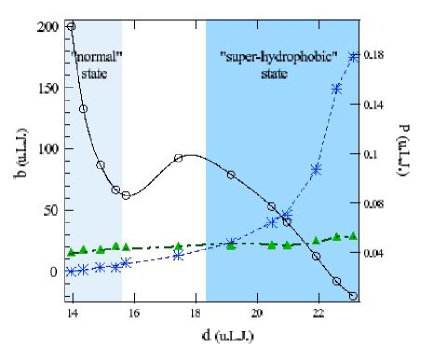
Figure 4: Evolution of the slip length $b$ as a function of the distance $d$ between the walls. The triangles ($\triangle$) represent the values of the slip lengths on the smooth wall, the stars ($\ast$) represent the values of the slip lengths on the rough wall, characterized by periodic grooves of height $h=10.7\ \sigma$, width $a=5\ \sigma$, periodicity $L=19.7\ \sigma$ and $c_{FS}=0.5$ (Lennard-Jones units). The flow is parallel to the grooves. The circles ($\circ$) indicate the value of the pressure (scale on the right of the figure). The lines are guides for the eye.

We present in figure 4 the evolution of the slip lengths on the smooth wall and on the rough wall, with the distance between the walls, together with the measured pressure (here the number of molecules per cell is fixed).

The results in figure 4 were obtained for a velocity parallel to the grooves. We have performed the same analysis for a velocity perpendicular to the grooves and obtained very similar results, which typically differ by a numerical constant (the slip in the direction perpendicular to the grooves being less pronounced than in the direction parallel to the grooves, as expected). In order to simplify the discussion, we will only present in the following the results for a liquid flowing parallel to the grooves.

As mentioned above, in the normal state, the roughness is found to reduce the slip. The slip length in the “normal” state is lower on the rough wall than on the smooth wall. On the other hand, in the “super-hydrophobic” state, roughness considerably enhances the slip length. In the “super-hydrophobic” state, one observes a strong dependence of the slip length with the pressure, an effect which can be correlated to the strong dependence of the shape of the liquid/vapor interface with the pressure. Indeed, as the pressure decreases, the interface changes from an incurvated shape in the grooves to a flat shape laying on the top of the roughness.

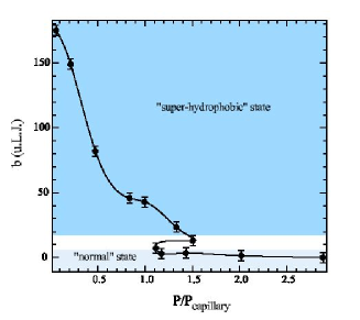
Figure 5: Evolution of the slip length (in Lennard-Jones units) as a function of $P/P_{capillary}$ for the same geometry as in figure 4.

In order to compare with experiments, it is more convenient to plot the slip length as a function of pressure (figure 5). In this figure the pressure is made dimensionless using the capillary pressure defined in equation (4). ¿From this kind of representation one may expect to be able to estimate the slip length for a specific roughness geometry, knowing the pressure of the system. From this figure, it is already obvious that small changes in the pressure induce very large difference in the measured slip length.

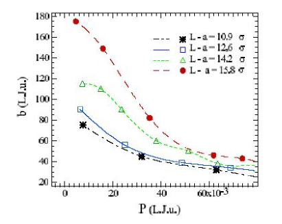
Figure 6: Evolution of the slip length $b$ as a function of $P$ (Lennard-Jones units) for grooves of different width $L-a$ and same height $h=9.6\ \sigma$. We only represent the slip lengths in the “super-hydrophobic” states.

We now turn to the influence of the geometry of the roughness on the slip length. We mainly focus on the role of the groove’s width. Figure 6 represents the evolution of the slip length as a function of the pressure for various widths of the grooves (keeping their height constant in this case). For a given pressure the slip length increases with the width of the grooves. This point can be easily understood. A wider groove implies a larger area of liquid/vapor interface, leading to a lower friction at the interface. From this figure we also note that small variations in the geometry of the grooves can lead to very large variations in the slip lengths. This fact could explain the great variability observed in the experimental results. Small differences in the state of the surfaces used in experiments could lead to huge differences on the slip lengths.

II.3 Conclusions and hydrodynamic description

At this stage we can draw a few general conclusions. On the basis of MD simulations we have shown that the surface roughness is a key factor in understanding the slippage of fluids on (hydrophobic) solid surfaces. Depending on the applied pressure a dewetting transition is found, which conversely enhances considerably the slip length at the surface.

We now try to rationalize this effect at the level of continuum hydrodynamics, in order to capture the dependence of the slip lengths as a function of the periodicity of the roughness. Indeed, in the dewetted state the liquid/wall interface takes the form of a succession of stripes, alternating a liquid-solid interface with a liquid-vapor interface. At the most simple level, the surface can be modelled as stripes with different slip lengths. To this end, we develop a macroscopic description of the hydrodynamic flow on a microscopically heterogeneous surface, characterized by a spatially varying slip length.

III Macroscopic approach : flow over a surface with a heterogeneous microscopic boundary condition

III.1 Introduction

We study here the influence of a microscopic heterogeneous h.b.c. on the macroscopic scale. Our aim is to define a macroscopic slip length corresponding to a heterogeneous microscopic h.b.c., with a spatially varying value of the slip length. We therefore consider a semi-infinite situation, where a shear flow, with a given shear rate $\dot{\gamma}$, is imposed at infinity. Using hydrodynamics, we show that far from the heterogeneous interface, that is to say for distances larger than the characteristic size of the structure, an effective slip length can be defined, which depends on the underlying “microscopic” slip heterogeneity.

We model the composite surface by a planar surface ($Oxy$ plane) characterized by a local slip length $b(x,y)$ function of the in plane coordinates $(x,y)$. Relying on the microscopic results of Molecular Dynamics, one may assume for instance that $b$ is locally very high over a vapor bubble and much lower elsewhere (for simple models, we may consider respectively infinite and zero slip lengths). The characteristics of the flow far away from the surface can then be determined by solving the hydrodynamic equations with the h.b.c. locally given by $b(x,y)$. Such an approach has been previously used to study local slipping heterogeneities of a simple geometric shape : periodic stripes parallel or perpendicular to the flow, corresponding to the alternance of a no slip boundary condition and an infinite slip. Philip has studied stripes parallel to the flow in a circular pipe of radius $R$ Philip . When $R\rightarrow\infty$, this configuration is the same as considering a flow at infinite over a plane, which is the situation studied here. In this limit, he obtains for the macroscopic slip length

$$B_{//}=\frac{L}{\pi}\ \textrm{ln}\ \left(\frac{1}{\textrm{cos}\left(\zeta\frac{\pi}{2}\right)}\right)$$ (5)

where $L$ is the periodicity of the pattern and $\zeta$ is the fraction of the surface where the slip length is infinite.

Lauga and Stone have established the expression of the macroscopic slip length for similar conditions than Philip (flow in a pipe of radius $R$ with $\zeta$ the fraction of infinite slip), but with a pattern perpendicular to the flow lauga . When $R\rightarrow\infty$, their expression for the macroscopic slip length reduces to

$$B_{\bot}=\ \frac{L}{2\pi}\ \textrm{ln}\ \left(\frac{1}{\textrm{cos}\left(\zeta\frac{\pi}{2}\right)}\right)\ .$$ (6)

We are interested here in a more general situation, involving an arbitrary pattern (both in geometry and magnitude) of the microscopic slip length.

III.2 Geometry and hydrodynamic equations

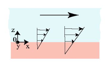
Figure 7: Schematic representation of the velocity field of the liquid for $z>0$, for a flow in the $x$ direction.

We consider an incompressible simple liquid occupying the half-space $z>0$, with an imposed shear stress $\dot{\gamma}$ in the $x$ direction and flowing over a fixed solid plane located in $z=0$ as shown in figure 7.

We now consider a stationary regime at low Reynolds number so that the Navier-Stokes equations can be written as

$$\left\{\begin{array}[]{rl}\eta{\bf\nabla}^{2}\bf{U}&=\bf{\nabla}\ P\\ \bf{\nabla}\cdot(\bf{U})&=0\end{array}\right.,$$ (7)

where $\bf{U}$ is the velocity vector, $P$ is the pressure and $\eta$ the viscosity of the liquid. The boundary conditions are defined as follows :

$\bullet$ at $z=0$ : a given local slip boundary condition $b(x,y)$ which is a function of the in plane coordinate.

$$\left\{\begin{array}[]{rl}b(x,y)\left.\frac{\partial{U}_{x}}{\partial z}\right|_{z=0}&=U_{x}(x;y;z=0)\\ \\ b(x,y)\left.\frac{\partial U_{y}}{\partial z}\right|_{z=0}&={U}_{y}(x;y;z=0)\\ \\ {U}_{z}(x;y;z=0)&=0\end{array}\right.$$ (8)

$\bullet$ for z $\rightarrow\infty$ :

$${\partial{{\bf U}}\over{\partial z}}=\dot{\gamma}{\bf e}_{x}$$ (9)

The effective slip length is defined in terms of the asymptotic velocity field, ${\bf U}$, solution of the above equations. In the $z\rightarrow\infty$ limit, one expects

$${\bf U}={\bf U}_{S}+\dot{\gamma}z\bf{e}_{x}=(\alpha+\dot{\gamma}z)\bf{e}_{x}+\beta{\bf e}_{y},$$ (10)

where ${\bf U}_{S}$ defines the “effective” velocity slip on the wall, with components {$\alpha,\beta$}: ${\bf U}_{S}$ is a constant velocity vector (independent of $x$ and $y$), parallel to the wall, which defines the macroscopic slip vector at the wall. The hydrodynamic equations (7) and the boundary conditions being linear, ${\bf U}_{S}$ must be proportional to $\dot{\gamma}$. The macroscopic slip lengths are then defined as $B_{x}=\alpha/\dot{\gamma}$ and $B_{y}=\beta/\dot{\gamma}$, here associated with a flow in the $x$ direction.

To solve this problem we introduce a new vector field

$${\bf V}={\bf U}-\dot{\gamma}z{\bf e}_{x}$$ (11)

and eliminate the pressure by using the vorticity

$${\mbox{\boldmath$\boldmath{\omega}$\unboldmath}}={\nabla}\times\bf{V}$$ (12)

The system (7) can be rewritten as :

$$\left\{\begin{array}[]{rl}\nabla^{2}\mbox{\boldmath$\boldmath{\omega}$\unboldmath}&=\bf{0}\\ \bf{\nabla}\cdot({\bf V})&=0\end{array}\right.$$ (13)

We consider a periodic pattern, with periodicity $L$ in both directions. Dimensionless variables (starred in the notations) are defined as

$$\left.\begin{array}[]{l}\displaystyle{x=x^{\ast}\frac{L}{2\pi}}\ ;\ \displaystyle y=y^{\ast}\frac{L}{2\pi}\ ;\ \displaystyle z=z^{\ast}\frac{L}{2\pi}\ ;\\ \\ b=b{}^{\ast}\frac{L}{2\pi}\ ;\\ \\ V=V{}^{\ast}\dot{\gamma}\frac{L}{2\pi}\ ;\ \displaystyle\omega=\omega^{\ast}\dot{\gamma}\ ;\\ \displaystyle\alpha=\alpha^{\ast}\dot{\gamma}\frac{L}{2\pi}\ ;\ \displaystyle\beta=\beta^{\ast}\dot{\gamma}\frac{L}{2\pi};\end{array}\right|$$ (14)

To simplify notations, we will drop the stars on the variables in the following, and all length and velocity variables must be understood as being rescaled by the periodicity of the pattern. The description of the resolution of equations (13) with h.b.c. (8) is given in the appendix, where we show that the system can be conveniently rewritten in terms of the 2D Fourier components of the various fields in the $x,y$ plane (we do not consider the Fourier transform in the $z$ direction):
For $\vec{q}\neq 0$ :

$$\left\{\begin{array}[]{rl}\left[\hat{b}\circ\underline{\hat{\omega}}_{y}\right]({\bf q})+\hat{b}({\bf q})&=\frac{q_{x}}{2q^{3}}\left(q_{x}\underline{\hat{\omega}}_{y}({\bf q})-q_{y}\underline{\hat{\omega}}_{x}({\bf q})\right)-\frac{\underline{\hat{\omega}}_{y}({\bf q})}{q}\\ -\left[\hat{b}\circ\underline{\hat{\omega}}_{x}\right]({\bf q})&=\frac{q_{y}}{2q^{3}}\left(q_{x}\underline{\hat{\omega}}_{y}({\bf q})-q_{y}\underline{\hat{\omega}}_{x}({\bf q})\right)+\frac{\underline{\hat{\omega}}_{x}({\bf q})}{q}\end{array}\right.$$ (15)

For $q=0$ and $z=0$ :

$$\left\{\begin{array}[]{rl}\left[\hat{b}\circ\hat{\omega}_{y}\right]({\bf q}={\bf 0})+\hat{b}({\bf q}={\bf 0})&=\alpha\\ -\left[\hat{b}\circ\hat{\omega}_{x}\right]({\bf q}={\bf 0})&=\beta\\ \end{array}\right.$$ (16)

where the notation “$\circ$” stands for the convolution product.

The previous system for $\underline{\hat{\omega}}_{x}({\bf q})$ and $\underline{\hat{\omega}}_{y}({\bf q})$, in equation (15), is solved numerically via a matrix inversion. The macroscopic slip lengths, $B_{x}$ and $B_{y}$, defined in terms of $\alpha$ and $\beta$, are then deduced by substituting this solution into (16). Calculation details are given in the appendix.

In the following section we present the results obtained for various patterns of the microscopic hydrodynamic boundary condition.

III.3 Alternating stripes with perfect slip and no-slip h.b.c.

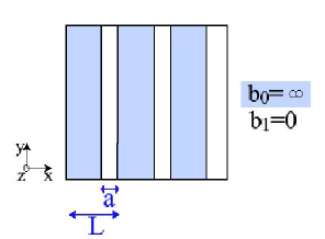
Figure 8: Schematic representation of the microscopic hydrodynamic boundary condition, alternance of strips of no-slip and perfect slip.

As sketched in figure 8, we consider a succession of stripes of width $a$ characterized by a vanishing slip length ($b_{1}=0$), and stripes of width $L-a$ with an infinite slip length ($b_{0}\rightarrow\infty$). The fraction of the surface with slippage is $\zeta=(L-a)/L$. We can consider stripes in any direction with respect to the flow, but we will mainly focus on the case of stripes parallel or perpendicular to the flow. This system corresponds obviously to a “model” experimental situation corresponding to a succession of grooves with vapor bubbles (slipping stripes) and rough strips (non slipping stripes). We present below the results for the effective macroscopic slip length $B$ in this situation.

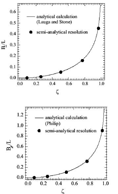
Figure 9: We consider an succession of stripes of width $a$ where the microscopic slip length is equal to zero ($b_{1}=0$) and strips of width $L-a$ with an infinite microscopic slip length ($b_{0}\rightarrow\infty$) and represent the evolution of the macroscopic slip length $B$ as a function of $\zeta$ ($\zeta$ is the fraction of the surface with a microscopic infinite slippage, $\zeta=(L-a)/L$). The curves represent the analytical calculations and the dots the numerical resolution (top: flow perpendicular to the strips, bottom : flow parallel to the strips.)

First we study the influence of the fraction of the slipping surface, $\zeta$, on the macroscopic slip length . This case is a benchmark for our calculation since in this specific situation we can compare our results with those obtained by Philip Philip and Stone and Lauga lauga in the limit of a cylinder with an infinite radius $R\ \rightarrow\ \infty$ lauga ; Philip . As shown on figure 9, our approach is in excellent agreement with their analytical results. This validates the semi-analytical approach developed here.

An interesting result emerging from the calculation in this specific geometry, is that a small percentage of non slipping surface ($1-\zeta\sim 0$) is enough to decrease considerably the effective slip : even for $\zeta=98.5\%$, $B$ is only a slightly larger than the size of the pattern of heterogeneity $L$ (here with a shear parallel to the pattern).

III.4 Alternating stripes of no-slip and partial slip h.b.c.

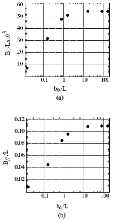
Figure 10: Macroscopic slip length $B$ on a surface composed of alternating stripes with slip length $b_{0}$ and vanishing slip length, for $\zeta=50\%$. On figure (a), the shear flow is perpendicular to the slipping stripes; on figure (b), the shear flow is parallel to the slipping stripes (note the change of vertical scale).

We now consider a different situation, with a surface composed of alternating non slipping stripes ($b_{1}=0$), and stripes with partial slip h.b.c., characterized by a slip length $b_{0}$. The surface fraction with slip length $b_{0}$ is again defined as $\zeta$. Our semi-analytical approach allows to consider any value of $b_{0}$, and extends therefore the results available in the literature, which are restricted to the $b_{0}=\infty$ case. We first present the results for $\zeta=50\%$. We have plotted in figure 10 the evolution of the macroscopic slip length as a function the microscopic slip length $b_{0}$ in the case of a flow parallel or perpendicular to the strip pattern. The main observations are :

• For low values of $b_{0}$ ($b_{0}<L$), the macroscopic slip length $B$ increases linearly with $b_{0}$ (of the order $b_{0}/4$ for the percentage of the slipping surface considered).

• For high values of $b_{0}$, ($b_{0}\ >\ 10L$) B asymptotically tends to a limiting value that is a fraction of the periodicity (around $L/10$ for a flow parallel to the strips and $L/20$ for a flow perpendicular to the strips).

The important point is that in the present $b_{1}=0$ case, the macroscopic slip length $B$ is fixed by the smallest of the two lengths $b_{0}$ and $L$.

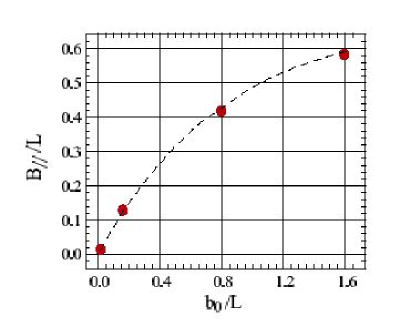
Figure 11: Macroscopic slip length $B$ on a surface composed of alternating stripes with slip length $b_{0}$ and vanishing slip length, as a function of the microscopic slip length $b_{0}$, for $\zeta=97\%$. The shear flow is parallel the slipping strips.

The same conclusions hold for larger values of $\zeta$. Figure 11 shows the results obtained for the effective slip length in the direction parallel to the stripe, $B_{\parallel}$, for a surface with a fraction $\zeta=97\%$ characterized by a slip length $b_{0}$. Due to numerical limitations, we could only study slip lengths $b_{0}/L<2$. The results are similar to those obtained at $\zeta=50\%$.

III.5 Alternating stripes of infinite slip and partial slip h.b.c.

We now consider a succession of stripes with an infinite slip length ($b_{0}\ \rightarrow\ \infty$) and stripes with a finite slip length $b_{1}$ (now with a non vanishing $b_{1}$). Obviously, this configuration is expected to model the situation considered in the first part of this work, specifically in the “super-hydrophobic” state. We have shown in the first part of this work that the interface between the liquid and the rough surface takes, in this state, the form of a succession of liquid-solid stripes, characterized by a finite slip length ($b_{1}\sim 20\sigma$, with $\sigma$ the molecular diameter), and liquid-vapor stripes, a priori characterized by an infinite slip length. We come back to this assumption in the following.

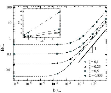
Figure 12: Macroscopic slip length $B$ on a surface composed of alternating stripes with slip length $b_{1}$ and infinite slip length, as a function of the microscopic slip length $b_{1}$. $B$ is computed for a shear parallel the slipping strips and for different values of $\zeta$. Dotted lines are a guide for the eye. In the inset the same points are plotted on a linear scale. The dashed lines are linear fits to the measured values of $B$.

Figure 12 shows the evolution of the macroscopic slip length $B$ as a function of the microscopic slip length $b_{1}$ for different fractions $\zeta$ of the slipping surface ($\zeta$ is defined here as the fraction of the surface with an infinite microscopic slip length, the rest of the surface having a finite slip length $b_{1}$). As shown on this figure, For $b_{1}>L$, the effective slip length $B$ evolves linearly with $b_{1}$ for all the fractions $\zeta$. On the other hand, one finds that for $b_{1}=0$ or $b_{1}\ll L$ the macroscopic slip length is fixed by the heterogeneity’s periodicity $L$, in agreement with the result of the section III.3 (for $b_{1}=0$ and $b_{0}\rightarrow\infty$). The important conclusion we can draw from these results is that in this geometry, with stripes of infinite slip length and finite slip length, the value of the macroscopic slip length is determined by the largest of the finite lengths : $b_{1}$ or $L$.

A simple phenomenological model can be formulated to explain the linearity with $b_{1}$ in the case $b_{1}>L$. We introduce the interfacial friction coefficient $\lambda$, defined by writing the continuity of the tangential stress $\sigma_{s}$ at the solid-liquid interface :

$$\sigma_{s}=\eta\,\frac{\partial\textrm{V}}{\partial z}\ =\ \lambda\textrm{V}_{s}$$

where $\eta$ is the viscosity of the liquid and V_s the velocity slip. The interfacial friction $\lambda$ coefficient is then related to the slip length $b$ by:

$$\lambda=\frac{\eta}{b}$$

The effective friction coefficient $\Lambda=\frac{\eta}{B}$ can be interpreted as the averaged friction over the different strips, and we obtain accordingly the following result for the effective macroscopic slip length as a function of the microscopic ones :

$$\frac{1}{B}=\frac{\zeta}{b_{0}}+\frac{1-\zeta}{b_{1}}\ ,$$ (17)

which is similar to the addition rule for resistors in parallel.

In the case $b_{0}\ \rightarrow\ \infty$, we expect :

$$B=\frac{b_{1}}{1-\zeta}$$ (18)

We have checked the linear dependance of $B$ with $b_{1}$ as well as the dependance with $\zeta$ (table 1) and we find that the relation 18 is very well verified for $b_{1}>L$. It is important to emphasize that its validity is limited to the case where both the slip lengths, $b_{0}$ and $b_{1}$ are larger than the roughness periodicity $L$. Note however that in practice, this relationship is valid down to $b_{1}>0.1L$ (see figure 12).

For $b_{1}\ll L$ or $b_{1}=0$ the friction coefficient tends to diverge over the strip and the model does not apply. Physically one may attribute this failure in this limit to the fact that the flow is strongly perturbed (compared to the asymptotic form) on the poorly slipping stripes ($b_{1}\ll L$). This is not taken into account in the simple argument leading to Eq. (18).

III.6 Comparison to Molecular Dynamics results

We are now in a position to compare the hydrodynamic predictions to the MD results. We focus on the super-hydrophobic state where the measured slip length is much larger than the bare slip length $b_{1}$ on the smooth surface. In order to make the comparison with the macroscopic approach, it is necessary to specify the local slip lengths on the top of the roughness (solid-liquid interface) and at the liquid-vapor interface on the grooves.

The analysis of the local profiles of velocity suggests an infinite slip length at the liquid-vapor interface ($b_{0}=\infty$), over a stripe of width $L-a$. For the slip length on the solid-liquid interface, on the top of the roughness, we take the value of the slip length $b_{smooth}$ obtained on a smooth wall at the same pressure ($b_{1}=b_{smooth}$ over a strip of width $a$). We only present the results in the case of shear parallel to the grooves. As we have mentioned before the slip length of a confined liquid depends on the pressure while there is no pressure dependence in the macroscopic approach. To introduce the pressure in the macroscopic approach we take into account the dependence of $b_{1}=b_{smooth}$ with the pressure. This dependence is measured independently in the simulations and depicted e.g. in figure 4.

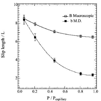
Figure 13: Comparison between MD measures of the slip length in the superhydrophobic state, and the macroscopic prediction of the slip length $B$ as a function of the pressure. The shear is parallel the slipping stripes. The macroscopic estimate assumes alternating stripes with finite slip length $b_{1}$ and infinite slip length; $b_{1}$ is accordingly identified with $b_{smooth}(P)$ the pressure dependent slip length on a smooth (and flat) solid surface, as measured independently in MD simulations. The percentage of the surface with an infinite slip length (macroscopic simulation) is identified as the percentage of the surface with a liquid-vapor interface (in MD simulations) : here $\zeta=83.3\%$. Lines are just a guide for the eyes.

The macroscopic slip length B is then computed using the macroscopic approach above, as a function of the pressure, in the case of alternated stripes with infinite slip length ($b_{0}=\infty$) and stripes with slip length $b_{1}=b_{smooth}(P)$. We compare these predictions with those obtained by molecular dynamic simulations with the same fraction $\zeta$ of surface with an infinite slip length. In figure 13, we compare the slip length $b$ obtained in MD simulations for various pressures with the macroscopic slip length $B$ computed along the lines described above. The perfectly slipping surface fraction is $\zeta=83.3\%$. The pressure is made dimensionless using the capillary pressure.

A few comments are in order.

• For low reduced pressures, $P/P_{cap}<.2$, there is a good and even quantitative agreement between the MD results and hydrodynamic predictions. This suggests that the hydrodynamic prediction, with a surface patterned with stripes characterized by infinite slip lengths and finite slip lengths, does capture the essential ingredients of heterogeneous slippage in the super-hydrophobic state.

• Nevertheless we see from figure 13 that this agreement deteriorates when the pressure approaches the capillary pressure, $P_{cap}$. In particular, the dependence of the slip length on the pressure is more pronounced in the case of the molecular dynamics simulations than in the macroscopic approach.

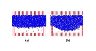
Figure 14: Transverse views of the atomic configuration for the same geometry as the one studied on figure 13 for (a) P/P${}_{\textrm{capillary}}$=0.4 and (b) P/P${}_{\textrm{capillary}}$=0.9.

A possible explanation for this difference is related to the geometry of the liquid-vapor interface which evolves as the pressure reaches $P_{cap}$, an ingredient which is not taken into account in the macroscopic approach. Figure 14 shows the evolution of the shape of the liquid-vapor interface, as measured in MD simulations. As can be seen from this figure, this interface strongly depends on the pressure and takes a curved shape for pressure close to $P_{cap}$. This suggests that the assumption of a plane liquid-vapor interface in the macroscopic approach in not appropriate at high pressure. The difference between the MD and hydrodynamic results indicates that the curved surface induces a supplementary dissipation as compared to the flat liquid-vapor interface, resulting in a lower effective slip length. Indeed, at high pressure, the liquid penetrates in the groove so that the flow is characterized by an increase of the velocity gradients compared to the low pressure case. These velocity gradients lead to a supplementary dissipation as compared to the flat interface, which could explain the difference between the two approaches at pressures close to the capillary pressure.

To conclude this section, this analysis points out the growing importance of the shape of the interface on the global friction at the interface, as pressure is increased.

IV Conclusions and perspectives

In this paper, we have considered the effect of surface heterogeneity on the slippage of fluid. Two approaches have been followed. First, we have used MD simulations to measure slip lengths on rough hydrophobic surfaces. A dewetting transition, leading to a super-hydrophobic state, is exhibited at small pressure, and leads to very large slippage of the fluid on this composite interface. Our results therefore confirm that mesoscopic roughness at the solid liquid interface can drastically modify the interfacial flow properties, in the same manner as it affects static wetting properties. Then on the basis of continuum hydrodynamics, we have proposed a macroscopic estimate of the effective slip length associated with a surface characterized by a heterogeneous slip length pattern. This (semi-analytical) approach has enabled us to determine the important factors controlling the effective slip length. In particular we have characterized the effective slip length $B$ for a surface with a striped microscopic hydrodynamic boundary condition characterized by slip lengths $b_{0}$ and $b_{1}$ with periodicity $L$. A few “rules of thumbs” emerge from this analysis :

• for $b_{1}=0$, the effective slip length $B$ is controlled by the smallest of the two lengths, $b_{0}$ or $L$;

• in the case where both slip lengths $b_{0}$ and $b_{1}$ are larger than the periodicity $L$, the effective slip length $B$ can be approximated by a “inverse law”

  $$\frac{1}{B}=\frac{\zeta}{b_{0}}+\frac{1-\zeta}{b_{1}}$$ (19)

  with $\zeta$ the surface fraction with slip length $b_{0}$. In practice, we found that this relationship holds down to $b_{0},b_{1}>{1\over 10}L$.

In this paper, we present results on the effective slip length $B$ associated with a surface formed by alternating stripes of different microscopic hydrodynamic boundary condition. However our results can be extended to more complex slipping patterns, relevant to experimental systems. As an example, surface patterns such as squares or dots can be easily implemented within our semi-analytical approach. Note that such microscopic patterns can not be solved in an analytical way.

We have then compared the results obtained within the two approaches, MD results and hydrodynamic description. While the hydrodynamic approach reproduces quantitatively the MD results for small pressures, a discrepancy between the two approaches is exhibited at large pressures, close to the dewetting transition. This points out the importance of the shape of the liquid-vapor interface in the “super-hydrophobic” state on the dissipation at the interface. The curvature of the liquid-vapor interface leads to a supplementary dissipation on the liquid-vapor interface.

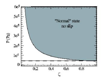
Figure 15: Evolution of the capillary pressure as a function of $\zeta$ ($P_{capillary}=\frac{-2\gamma_{lv}\cos{\theta}}{\zeta L}$) for $\theta=105^{\circ}$and $\gamma_{lv}=72$ mN/m. In the grey zone the pressure is higher than the capillary pressure, the liquid is in the “normal” state, it is not possible to have high values of the slip length. The dashed lines corresponds to the pressure drop for microfluidic experiments. The intersection between this dashed line and the capillary pressure’s curve gives the upper value of $\zeta$, here $\zeta=0.9$.

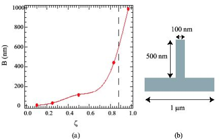
Figure 16: (a) Evolution of the macroscopic slip length $B$ as a function of $\zeta$, when $\zeta$ % of the surface has an infinite slip length and ($1-\zeta$) % of the surface has a slip length of 20 nm (the periodicity is $L=1\mu$m). The vertical dashed corresponds to the maximum value of $\zeta$ possible as explained on figure 15. (b) Kind of structure that can lead to slip lengths up to 600 nm.

Eventually, as an example of application of the previous macroscopic and molecular dynamic approaches, we now apply these results to design a potentially highly slipping surface. This is motivated by potential applications, especially in microfluidics. The motivation to design highly slipping surfaces is linked in particular to the development of flat velocity profiles within microchannel, aiming at reducing the dispersion in the transport of different species. Such a flat profile can be obtained using a pressure drop flow with a highly slipping channel. The studies we have presented show that high slippage can be achieved using a hydrophobic channel with “appropriate” roughness. We now have to design this “appropriate” roughness. For microfluidic applications, let us assume a periodicity $L=1\mu m$. We have to determine the percentage of the surface $\zeta=\frac{L-a}{L}$ which has an infinite slip length. We assume that the slip length of the liquid over the smooth hydrophobic solid is about 20 nm. Using the macroscopic approach, we can represent the evolution of the macroscopic slip length $B$ as a function of $\zeta$. Since $B$ is required to be the largest, one can naively think that we should have the largest possible $\zeta$. However, as we have seen with the molecular dynamic simulations, high slippage requires the liquid to be in a “super-hydrophobic” state, so that it can “dewet” over the roughness, giving infinite slip length at the liquid-vapor interface. For this, the pressure has to be roughly lower than the capillary pressure (as long as the grooves are deep enough). This capillary pressure can be expressed in terms of $\zeta$ : $P_{cap}=\frac{-2\gamma_{lv}\cos{\theta}}{\zeta L}$. If we consider a pressure drop experiment in a microfluidic channel, the pressure drop that has to be applied is typically of $0.4\cdot 10^{5}$ Pa cheng2002 . As represented on figure 15 this gives us the upper limit of $\zeta$ ($\zeta=0.88$ in our example). Therefore, if we consider grooves of 100 nm width and periodicity 1 $\mu$m one may expect slip length as large as 600 nm (figure 16). This description does not determine the height of the grooves, but the main constraint for them is to be high enough, so that the capillary pressure does actually tune the transition between the normal and the super-hydrophobic state (of course their height is also limited by the technological fabrication possibilities); typically here a height of 500 nm should be appropriate.

In summary, use of surfaces patterned at the nanometer scale, and treated to produce a ’water repellent’ like effect, appears to be a promising way towards devices that would allow flow of liquids in small size channels with very small flow resistance.

Appendix: calculation details

Here we present in some detail the resolution of the stationary Stokes equation with a locally imposed slipping h.b.c.. We have defined in equation (11) the relative velocity field :

$${\bf V}={\bf U}-\dot{\gamma}z\bf{e}_{x}$$

which verifies the following boundary conditions :

$\bullet$ For $z=0$ :

$$\left\{\begin{array}[]{rl}{b(x,y)}\left(\left.\frac{\partial{V}_{x}}{\partial z}\right|_{z=0}+\dot{\gamma}\right)&={V}_{x}(x;y;z=0)\\ \\ {b(x,y)}\left.\frac{\partial{V}_{y}}{\partial z}\right|_{z=0}&={V}_{y}(x;y;z=0)\\ \\ {V}_{z}(x;y;z=0)&=0\end{array}\right.$$ (20)

$\bullet$ For $z\ \rightarrow\infty$ :

$${\bf V}=\alpha\bf{e}_{x}+\beta{\bf e}_{y}$$ (21)

We solve this problem by expanding the various fields in Fourier series, assuming for simplicity the dimensionless variables as defined in (14) and a pattern with periodicity 2$\pi$ in both the $x$ and $y$ direction. For that we use the following definition for the Fourier coefficients in $x$ and $y$ directions

$$\hat{{\bf V}}(q_{x};q_{y};z)=\frac{1}{(2\pi)^{2}}\int\int_{[-\pi;\pi]}e^{-i{\bf q}.\bf{r}}\bf{V}(x;y;z)dxdy$$ (22)

where ${\bf q}$ is a two dimensional wave vector, ${\bf q}=q_{x}\hat{{\bf e}_{x}}+q_{y}\hat{{\bf e}_{y}}$ with discretized values $q_{x,y}=n_{x,y}$. The vorticity ${\mbox{\boldmath$\boldmath{\omega}$\unboldmath}}={\nabla}\times{\bf V}$ can then be written in Fourier space as :

$$\left\{\begin{array}[]{rl}\hat{\omega}_{x}&=iq_{y}\hat{V}_{z}-\frac{\partial\hat{V}_{y}}{\partial z}\\ \\ \hat{\omega}_{y}&=\frac{\partial\hat{V}_{x}}{\partial z}-iq_{x}\hat{V}_{z}\\ \\ \hat{\omega}_{z}&=iq_{x}\hat{V}_{y}-iq_{y}\hat{V}_{x}\\ \end{array}\right.$$ (23)

We can deduce from equation (13) and from the fact that $\boldmath{\omega}$ must vanish as $z\rightarrow\infty$, that :

$$\left\{\begin{array}[]{rl}\hat{\omega}_{x}({\bf q};z)&=\underline{\hat{\omega}_{x}}({\bf q})e^{-qz}\\ \\ \hat{\omega}_{y}({\bf q};z)&=\underline{\hat{\omega}_{y}}({\bf q})e^{-qz}\\ \\ \hat{\omega}_{z}({\bf q};z)&=\underline{\hat{\omega}_{z}}({\bf q})e^{-qz}\\ \\ \end{array}\right.$$ (24)

By taking the Fourier transform of the h.b.c. (20), and taking into account that $\hat{V}_{z}(z=0)=0$, we obtain the system (25) for $q\neq 0$.

$$\left\{\begin{array}[]{rl}\left[\hat{b}\circ\underline{\hat{\omega}}_{y}\right]({\bf q})+\hat{b}({\bf q})&=\frac{q_{x}}{2q^{3}}\left(q_{x}\underline{\hat{\omega}}_{y}({\bf q})-q_{y}\underline{\hat{\omega}}_{x}({\bf q})\right)-\frac{\underline{\hat{\omega}}_{y}({\bf q})}{q}\\ -\left[\hat{b}\circ\underline{\hat{\omega}}_{x}\right]({\bf q})&=\frac{q_{y}}{2q^{3}}\left(q_{x}\underline{\hat{\omega}}_{y}({\bf q})-q_{y}\underline{\hat{\omega}}_{x}({\bf q})\right)+\frac{\underline{\hat{\omega}}_{x}({\bf q})}{q}\end{array}\right.$$ (25)

The Fourier transform of (20) gives for $q=0$

$$\left\{\begin{array}[]{rl}\left[\hat{b}\circ\hat{\omega}_{y}\right]({\bf q}=\bf{0})+\hat{b}({\bf q}=\bf{0})&=\alpha\\ -\left[\hat{b}\circ\hat{\omega}_{x}\right]({\bf q}=\bf{0})&=\beta\\ \end{array}\right.$$ (26)

where $\circ$ denotes a convolution sum.

By solving (25) for ${\omega}_{x}$ and ${\omega}_{y}$ and replacing into (26), we can determine $\alpha$ and $\beta$ and then the macroscopic slip length. Equations (25) only involve $\underline{\hat{\omega}}_{x}$, $\underline{\hat{\omega}}_{y}$ and $\hat{b}$. Since $\hat{b}$ is an input of the problem, it is then possible to determine $\underline{\hat{\omega}}_{x}$ and $\underline{\hat{\omega}}_{y}$.

This resolution of $\underline{\hat{\omega}}_{x}$ and $\underline{\hat{\omega}}_{y}$ can not usually be done analytically (except for very simple patterns of $b$) and a numerical approach is required. For that, we consider a discretization of the elementary cell (of size $(2\pi)^{2}$ in the real space) into $N^{2}$ nodes of coordinates :

$$\begin{split}(x_{k};y_{k})=\left(-\pi+k_{x}\frac{2\pi}{N};-\pi+k_{y}\frac{2\pi}{N}\right)\\ \quad\text{where}\quad(k_{x},k_{y})\in[0,N-1]^{2}\end{split}$$ (27)

The discretisation of real space implies periodicity in the Fourier space with period $N$. We then only consider the wave vectors ${\bf q}$ in the interval :

$$(q_{x};q_{y})\in[0,(N-1)]^{2}$$

By introducing the complex vector $\hat{\Omega}({\bf q})=\underline{\hat{\omega}}_{x}({\bf q})+j\underline{\hat{\omega}}_{y}({\bf q})$ and by making a judicious combination of the equations (25), the problem is reduced to a matrix system of the form :

$$\left(\begin{array}[]{c}M\end{array}\right)\left(\begin{array}[]{c}\Omega\end{array}\right)=\left(\begin{array}[]{c}B\end{array}\right)$$ (28)

where $\left(\Omega\right)$ is a vector of size 2($N^{2}$-1) involving only $\underline{\hat{\omega}}_{x}$ and $\underline{\hat{\omega}}_{y}$ , and $\left(B\right)$ is a vector of size 2($N^{2}$-1) that only involves the prescribed microscopic slip length $b$. The size of the matrix $\left(M\right)$ is 4$\times$($N^{2}$-1)², which increases rapidly with $N$. However, for most of the situation of interest, ($M$) remains a sparse matrix with many zero coefficients. The density of the matrix does actually depend on the pattern of the microscopic h.b.c.. For a strip pattern of microscopic h.b.c., for example, only 3 % of the elements of the matrix’ elements are non zero (this spareness actually results from the invariance by translation of the pattern in the direction of the stripes). This allows the implementation of efficient sparse matrix algorithms to solve equation (28). We typically consider N up to N=256 grid points both in $x$ and $y$ directions. The matrix (M) is then inverted using a conjugated gradient method well suited to the inversion of matrix of low densities.

“Real” value of $\zeta$	Value of $\zeta$ from the
	linear fit of $B$ ($\pm~{}2\%$)
	as a function of $b_{1}$
97	96.7
83.3	83.2
50	49.2
25	24.8
10	9.9

Table 1: Comparison of the “real” value of the fraction $\zeta$ and the value one get with a linear fit using the equation 18

References

- (1) V.D. Sobolev, N.V. Churaev and A.N. Somov. J. Colloid Interface Sci., 97(2): 574–581, 1984.
- (2) K. Watanabe and Y. Udagawa and H. Ugadawa J. Fluid Mech., 381 : 225-238, 1999.
- (3) O. Vinogradova International Journal of Mineral Processing, 56 (1-4) : 31-60, 1999.
- (4) R. Pit, H. Hervet, and L. Léger. Phys. Rev. Lett., 85(5) : 980-983, 2000.
- (5) J. Baudry, É. Charlaix, A. Tonck, and D. Mazuyer. Langmuir, 17 : 5232–5236, 2001.
- (6) V.S.J. Craig, C. Neto, and D.R.M. Williams. Phys. Rev. Lett., 87(5) : 054504(1–4), 2001.
- (7) Y. Zhu and S. Granick. Phys. Rev. Lett., 87 : 096105(1–4), 2001.
- (8) J.-T. Cheng and N. Giordano. Phys. Rev. E, 65 : 031206(1–5), 2002.
- (9) Y. Zhu and S. Granick. Phys. Rev. Lett., 88 : 106102(1–4), 2002.
- (10) D.C. Tretheway and C.D. Meinhart. Physics of Fluids, 14(3) : L9–L12, 2002.
- (11) E. Bonnacurso, M. Kappl and H.-S. Butt. Phys. Rev. Lett., 88 : art n°076103, 2002.
- (12) C. Cottin-Bizonne, S. Jurine, J. Baudry, J. Crassous, F. Restagno and É. Charlaix. Eur. Phys. J. E, 9, 47-53.
- (13) E. Bonaccurso, H.-J. Butt and V. S. Craig. Phys. Rev. Lett., 90 : art n°144501, 2003.
- (14) O.I. Vinogradova and G. E. Yabukov Langmuir, 19 : 1227-1234, 2003.
- (15) C.-H. Choi, K. Johan, A. Westin and K. S. Breuer Physics of Fluids, 15, 2897-29002
- (16) S. Richardson, J. Fluid Mech., 59 : 707-719, 1973.
- (17) J.-L. Barrat and L. Bocquet. Faraday discussions, 112 : 119–127, 1999.
- (18) J.-L. Barrat and L. Bocquet. Phys. Rev. Lett., 82 : 4671–4674, 1999.
- (19) P.A. Thompson and S.M. Troian. Nature(London), 389 : 360–362, 1997.
- (20) B. Lefevre, A. Saugey, J.-L. Barrat, L. Bocquet, E. Charlaix, P.-F. Gobin and G. Vigier J. Chem. Phys., 120 : 4927-4938, 2004.
- (21) C. Cottin-Bizonne, E. Charlaix, L. Bocquet, J.-L. Barrat Nature Materials, 2, 238, 2003.
- (22) J. R. Philip. J. App. Math. and Phys., 23 : 960-968, 1972.
- (23) E. Lauga and H. Stone J. Fluid Mech., 483 : 55-77, 2003.
- (24) J.W.G. Tyrell and P. Attard. Phys. Rev. Lett., 87(17) : 176104–(1–4), 2001.
- (25) P.G. de Gennes, C.R. Acad. Sc. Paris, 288, 219 (1979).